HAL Id: tel-03016351
https://hal.archives-ouvertes.fr/tel-03016351v2
Submitted on 6 Jan 2021
HAL is a multi-disciplinary open access
archive for the deposit and dissemination of
sci-entific research documents, whether they are
pub-lished or not. The documents may come from
teaching and research institutions in France or
L’archive ouverte pluridisciplinaire HAL, est
destinée au dépôt et à la diffusion de documents
scientifiques de niveau recherche, publiés ou non,
émanant des établissements d’enseignement et de
recherche français ou étrangers, des laboratoires
multiprocessor embedded systems
Petr Dobiáš
To cite this version:
Petr Dobiáš. Online fault tolerant task scheduling for real-time multiprocessor embedded systems.
Embedded Systems. Université Rennes 1, 2020. English. �NNT : 2020REN1S024�. �tel-03016351v2�
T
HÈSE DE DOCTORAT DE
ÉCOLE
DOCTORALE
N
O601
Mathématiques et Sciences et Technologies de l’Information et de la Communication Spécialité : Informatique
Par
Petr DOBIÁŠ
Contribution à l’ordonnancement dynamique, tolérant aux
fautes, de tâches pour les systèmes embarqués temps-réel
multiprocesseurs
Thèse présentée et soutenue à Lannion, le 2 octobre 2020
Unité de recherche : IRISA
Rapporteurs avant soutenance :
Alberto BOSIO Professeur des Universités, Ecole Centrale de Lyon, France
Arnaud VIRAZEL Maître de Conférences, Université de Montpellier, France
Composition du Jury :
Président : Bertrand GRANADO Professeur des Universités, Sorbonne Université, France
Examinateurs : Alberto BOSIO Professeur des Universités, Ecole Centrale de Lyon, France
Maryline CHETTO Professeur des Universités, Université de Nantes, France
Daniel CHILLET Professeur des Universités, Université de Rennes 1, France
Oliver SINNEN Associate Professor, University of Auckland, Nouvelle Zélande
Arnaud VIRAZEL Maître de Conférences, Université de Montpellier, France
Dir. de thèse : Emmanuel CASSEAU Professeur des Universités, Université de Rennes 1, France
R
ÉSUMÉ
La thèse se focalise sur le placement et l’ordonnancement dynamique des tâches sur les systèmes embarqués multiprocesseurs pour améliorer leur fiabilité tout en tenant compte des contraintes telles que le temps réel ou l’énergie. Les performances du système sont principalement évaluées par le nombre de tâches rejetées, la complexité de l’algorithme et donc sa durée d’exécution et la résilience estimée en injectant les fautes. Les contributions de la recherche sont dans les deux domaines suivants : l’approche d’ordonnancement dite de « primary/backup » et la fiabilité des petits satellites appelés CubeSats.Description de l’approche de « primary/backup »
L’approche de « primary et backup » (approche PB) considère que chaque tâche a deux copies identiques pour rendre le système tolérant aux fautes [61]. Ces copies sont placées sur deux processeurs différents entre le temps d’arrivée de la tâche et sa date limite d’exécution. La première copie nommée copie de « primary » est placée le plus tôt possible tandis que la deuxième copie appelée copie de « backup » est positionnée le plus tard possible. Pour améliorer l’ordonnancement, les copies de « backup » peuvent être chevauchées entre elles ou désallouées si les exécutions de leurs copies de « primary » respectives sont correctes. D’autres heuristiques pour l’approche PB ont été déjà présentées [61, 103, 144, 155]. Les fautes sont détectées par un mécanisme de détection qui signale leur occurrence.
Contributions à l’approche de « primary/backup »
Le but est de proposer des heuristiques subtiles pour réduire la durée d’exécution (mesurée à l’aide du nombre de comparaisons) de l’algorithme d’ordonnancement tout en évitant la détérioration des performances du système (évaluées par exemple par le taux de réjection, i.e. le nombre de tâches rejetées par rapport au nombre total de tâches). Les contributions à l’approche PB sont les suivantes :
— l’évaluation de la surcharge de cette approche ;
— la proposition d’une nouvelle stratégie d’allocation des processeurs qu’on nomme la « recherche jusqu’à la première solution trouvée – créneau après créneau » (FFSS SbS) et qu’on compare avec d’autres stratégies déjà existantes ;
— la proposition de trois nouvelles heuristiques : (i) la méthode de limitation du nombre de
compa-raisons, (ii) la méthode de limitation des fenêtres d’ordonnancement délimitant le temps pendant
lequel une copie peut être placée et (iii) la méthode de plusieurs essais d’ordonnancement ; — l’évaluation des performances de l’algorithme, en particulier en termes de nombre de comparaisons
par tâche et de taux de réjection, y compris avec l’injection des fautes ;
— la formulation mathématique du problème et la comparaison des résultats avec la solution optimale délivrée par le solveur CPLEX ;
— l’adaptation des algorithmes proposés ci-dessus pour des tâches indépendantes afin de placer des tâches dépendantes.
Analyses des résultats de l’approche de « primary/backup »
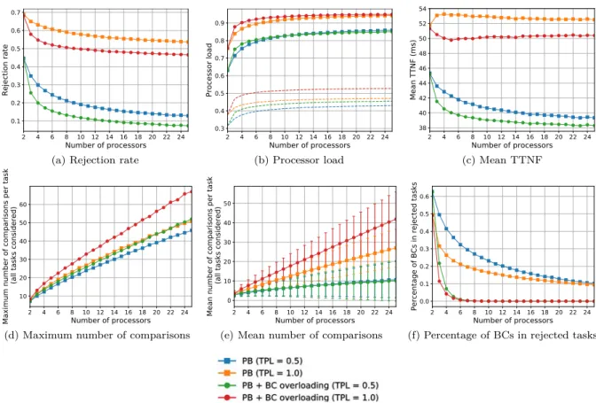
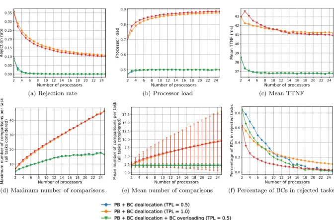
Les analyses des résultats pour les tâches indépendantes ont permis de conclure les points suivants. Le taux de réjection du système autorisant le chevauchement des copies de « backup » est réduit par rapport au système sans aucune technique particulière (par exemple de 14% pour un système avec 14 processeurs). En cas de la désallocation des copies de « backup », il est réduit encore davantage (par
Le surcoût de l’approche PB qui place deux copies de la même tâche (même si la copie de « backup » peut être désallouée) a été également évalué. Quand le nombre de processeurs augmente, le nombre de comparaisons par tâche pour trouver une place pour ses copies augmente également et la différence du nombre de comparaisons entre les systèmes sans et avec approche PB devient plus importante. Néanmoins, comme il y a plus de comparaisons effectuées, la probabilité de placer une tâche augmente et donc le taux de réjection du système tolérant aux fautes diminue et se rapproche de celui du système non-tolérant.
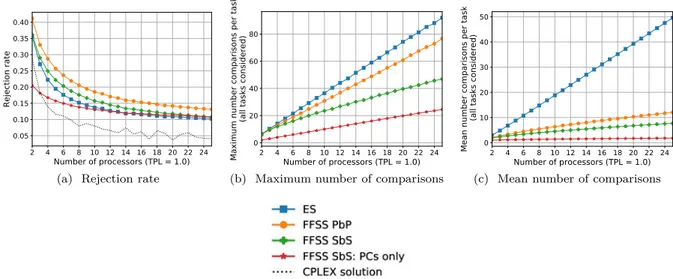
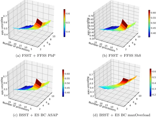
Ensuite, on compare les trois stratégies d’allocation des processeurs : la « recherche exhaustive » (ES), la « recherche jusqu’à la première solution trouvée – processeur après processeur » (FFSS PbP) et la « recherche jusqu’à la première solution trouvée – créneau après créneau » (FFSS SbS). L’ES a le taux de réjection le plus bas parmi toutes les stratégies mais ses nombres moyen et maximal de comparaisons par tâche sont au contraire les plus élevés. La méthode FFSS SbS est un bon compromis. Par exemple, le taux de réjection de FFSS SbS est de 12% plus élevé que celui d’ES pour un système avec 14 processeurs et son nombre maximal de comparaisons par tâche est considérablement inférieur par rapport à celui de FFSS PbP (29% pour un système avec 14 processeurs) et à celui d’ES (41% pour un système avec 14 processeurs). De plus, en comparant l’algorithme basé sur FFSS SbS à la solution optimale obtenue par un solveur CPLEX, on trouve qu’il est 2-compétitive.
Puis, deux techniques pour parcourir les processeurs sont étudiées : la « recherche basée sur les créneaux disponibles » (FSST) et la « recherche basée sur les débuts et les fins des copies déjà placées » (BSST). La méthode BSST + ES et la méthode FSST + ES ont des nombres similaires de tâches rejetées et BSST a besoin plus que deux fois plus de comparaisons que la FSST. Ainsi, BSST n’est pas une technique à choisir en termes de durée d’exécution de l’algorithme.
Après les analyses des stratégies d’allocation des processeurs et des techniques pour parcourir les processeurs, on s‘intéresse aux performances des heuristiques qu’on propose.
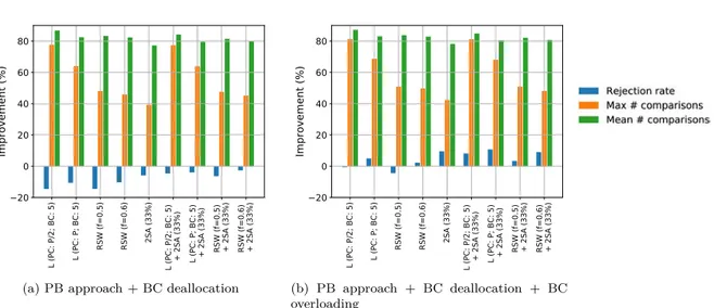
La méthode de limitation du nombre de comparaisons montre que la définition du seuil permet de réduire le nombre maximal des comparaisons. Par exemple, si ce seuil pour les copies de « primary » est fixé à P/2 comparaisons (où P est le nombre de processeurs) et celui pour les copies de « backup » est égal à 5 comparaisons, les nombres maximal et moyen des comparaisons par tâche respectivement diminuent de 62% et 34% tandis que le taux de réjection augmente seulement de 1,5% en comparant avec l’approche PB sans cette méthode.
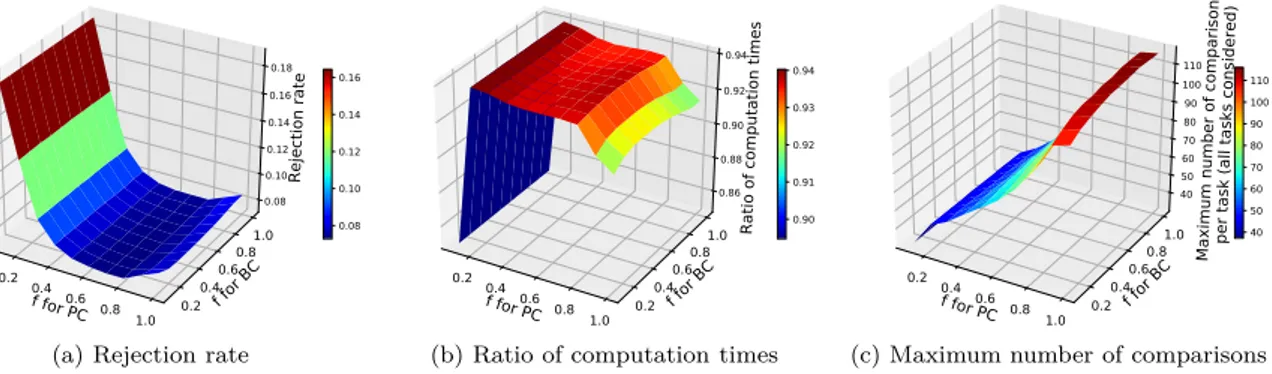
La méthode de limitation des fenêtres d’ordonnancement est aussi efficace pour réduire le nombre de comparaisons sans aggraver les performances du système. Un compromis raisonnable entre le nombre de comparaisons et le taux de réjection est obtenu pour la fraction de la fenêtre de tâche égale à 0,5 ou 0,6. La troisième heuristique proposée, plusieurs essais d’ordonnancement, vise à abaisser le taux de ré-jection des tâches. Les résultats montrent qu’il est inutile de réaliser plus que deux essais car, quand le nombre d’essais augmente, le taux de réjection ne diminue que marginalement et le nombre de comparai-sons par tâche augmente assez vite. Un bon compromis entre ces deux métriques est obtenu pour deux essais ayant lieu à 33% de la fenêtre de tâche. Dans ce cas-là, le taux de réjection décroît de 6,2%.
En comparant les heuristiques et leurs combinaisons en termes de taux de réjection et du nombre de comparaisons, on trouve que les meilleurs résultats sont obtenus pour : (i) la méthode de limitation du nombre de comparaisons utilisant deux essais à 33% de la fenêtre de tâche et (ii) la méthode de limitation du nombre de comparaisons. Dans le premier cas mentionné, le nombre de comparaisons diminue considérablement (valeur moyenne : 23% ; valeur maximale : 67%) et le taux de réjection est réduit de 4% par rapport à l’approche PB sans aucune technique d’amélioration.
Pour évaluer les performances en présence des fautes, l’algorithme proposé a été testé par l’injection
des fautes. On a constaté que les injections des fautes allant jusqu’à 1·10−3fautes par processeurs/ms ont
un impact minimal. Comme cette valeur est supérieure à la valeur estimée dans les conditions standard (2· 10−9fautes par processeurs/ms [47]) et à celle dans les conditions rudes (1·10−5fautes par processeurs/ms
[118]), l’algorithme peut donc être implémenté dans les systèmes exposés à l’environnement hostile. Afin de prolonger l’étude sur l’approche PB, l’algorithme proposé a été modifié pour gérer les tâches
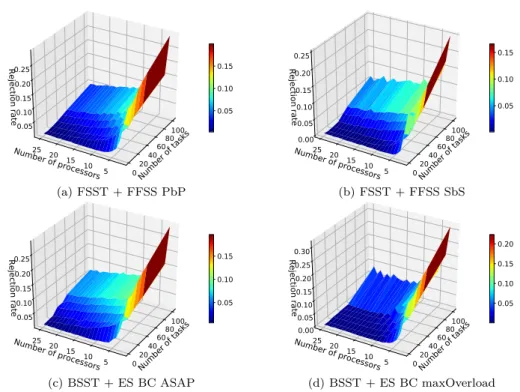
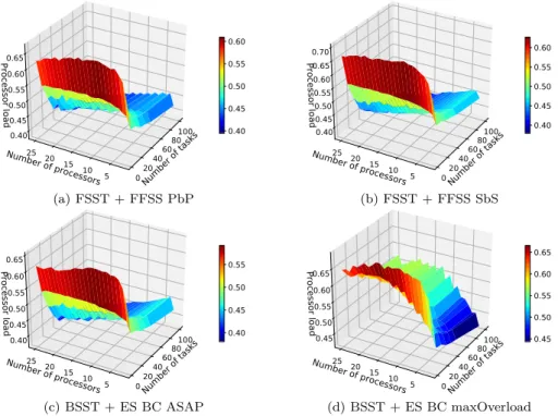
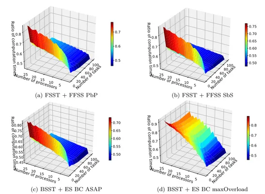
dépendantes modélisées par les graphes orientés acycliques (DAG). Les deux techniques pour parcourir les processeurs (FSST et BSST) combinées à trois stratégies d’allocation des processeurs (ES, FFSS PbP et FFSS SbS) ont été de nouveau comparées. Le nombre de comparaisons par DAG pour BSST + ES est considérablement plus élevé que pour les deux autres techniques (FSST + FFSS PbP et FSST + FFSS SbS) ce qui est dû au type de la recherche : exhaustive ou pas. Bien que la FFSS SbS et la FFSS PbP aient un taux de réjection similaire, la FFSS SbS nécessite plus de comparaisons. La méthode maximisant le chevauchement entre les copies de « backup » (BSST + ES maxOverload) a les meilleurs résultats en termes de taux de réjection mais au détriment de la durée d’exécution de l’algorithme, sauf pour les systèmes ayant peu de processeurs. L’injection des fautes a montré que l’algorithme proposé fonctionne bien même avec les taux d’injection des fautes supérieurs aux valeurs réelles dans les conditions difficiles.
Description des CubeSats
Les CubeSats sont les petits satellites envoyés dans l’orbite basse de la Terre avec des missions scientifiques. Leurs popularité augmente grâce à la standardisation qui réduit le budget et le temps de développement [52]. Ils sont composés d’un ou plusieurs cubes d’arête de 10 cm et de poids maximal de 1, 3 kg [108]. À bord, il y a en général plusieurs systèmes électroniques systèmes, comme l’ordinateur de bord, le système de la détermination d’attitude et de contrôle ou le système lié à la mission (partie scientifique).
Les CubeSats sont exposés aux particules chargées et aux radiations qui causent des effets singuliers, par exemple « Single Event Upset » (SEU) et des effets de dose, comme « Total Ionizing Dose » (TID) [89]. Il est donc nécessaire de concevoir des CubeSats plus robustes. Les méthodes de robustification ne sont pas de manière générale utilisées en raison des contraintes budgétaire, du temps de conception ou de l’espace disponible [55]. Par exemple, il y a 43% de CubeSats qui ne mettent pas en œuvre la redondance, technique classique au niveau matériel [54, 90]. En raison de contraintes spatiales, il est préférable d’utiliser les méthodes logicielles, comme les watchdogs ou les techniques protégeant les données [3, 36, 38].
Contributions aux CubeSats
Pour améliorer la fiabilité des CubeSats, on propose de regrouper tous les processeurs à bord sur une même carte ayant un seul système intégré. Même si cette modification peut paraître importante pour les CubeSats actuels, elle a été déjà réalisée avec succès à bord d’ArduSat avec 17 processeurs [58]. Ainsi, il sera plus facile de protéger les processeurs, par exemple en utilisant un blindage contre les radiations [30], et d’augmenter les chances de bon déroulement de la mission car si un processeur est défectueux, d’autres processeurs qui ne sont pas dédiés à un système donné (comme c’est le cas dans les CubeSats actuels) continuent à fonctionner.
Dans ce cadre-là, on a développé des algorithmes qui placent toutes les tâches (périodiques, sporadiques et apériodiques) à bord de CubeSat, détectent des fautes et prennent des mesures pour délivrer des résultats corrects. L’objectif est de minimiser le nombre de tâches rejetées en respectant les contraintes temporelles, énergétiques et la fiabilité. Ces algorithmes sont exécutés dynamiquement pour immédiate-ment réagir. Ils sont principaleimmédiate-ment dédiés aux CubeSats basés sur les processeurs commerciaux standard qui ne sont pas conçus pour l’utilisation dans l’espace contrairement aux processeurs durcis.
Les contributions dans le domaine des CubeSats sont les suivantes :
— l’évaluation des performances de trois algorithmes d’ordonnancement proposés, dont un tenant compte des contraintes énergétiques, en termes de taux de réjection, de nombre de recherches d’ordonnancement effectuées et de durée d’exécution d’algorithme ;
— la formulation mathématique du problème et la comparaison des résultats avec la solution optimale délivrée par le solveur CPLEX ;
— l’évaluation de la durée du fonctionnement du système en utilisant l’algorithme proposé prenant en compte les contraintes énergétiques ;
Analyses des résultats des CubeSats
L’algorithme appelé OneOff considère toutes les tâches comme apériodiques et l’algorithme nommé OneOff&Cyclic distingue les tâches périodiques et apériodiques. Tandis que ces deux algorithmes ne tiennent pas compte de contraintes énergétiques, l’algorithme OneOffEnergy les considère. Tous les algorithmes peuvent utiliser différentes stratégies de placement pour ordonner la queue des tâches.
Les performances de OneOff et OneOff&Cyclic ont été étudiés avec trois scénarios, dont deux proviennent de réels CubeSats. Les scénarios diffèrent par la charge du système et le rapport entre les tâches simples et doubles.
Les résultats montrent qu’il est inutile de considérer un système ayant plus de six processeurs car, si un stratégie d’ordonnancement est bien choisi, il n’y a pas de tâche rejetée. Ce choix permet donc d’éviter un système surdimensionné. De manière générale, les stratégies de placement "Earliest Deadline" pour OneOff et "Minimum Slack" pour OneOff&Cyclic minimisent bien la fonction objectif, i.e. le taux de réjection. Elles ont également de bonnes performances en termes de durée de l’ordonnancement.
Même s’il a été trouvé que OneOff&Cyclic fonctionne moins bien que OneOff, ce dernier algo-rithme peut très bien être utilisé dans d’autres applications avec beaucoup plus de profits (par exemple dans les systèmes embarqués avec les contraintes temporelles sévères) ayant moins de déclencheurs d’or-donnancement (moins de fautes, ou moins des tâches apériodiques ou moins de changements dans l’en-semble des tâches périodiques) que dans les applications étudiées.
Ainsi, les équipes construisant leurs propres CubeSats qui regroupent tous les processeurs sur une seule carte, devraient choisir plutôt OneOff si elles hésitent entre les deux algorithmes ne prenant pas en compte les contraintes énergétiques. Néanmoins, il serait mieux d’implémenter le troisième algorithme OneOffEnergy prenant également en compte les contraintes énergétiques.
OneOffEnergy profite de deux régimes du processeur (Run and Standby) pour réduire la consom-mation énergétique et fonctionne dans un des trois régimes (normal, safe et critical) suivant le niveau d’énergie disponible dans la batterie. Cet algorithme proposé a été évalué non seulement dans le cas des CubeSats mais aussi pour une autre application ayant des contraintes énergétiques.
Le bilan énergétique établi pour le Scénario APSS montre que la phase de communication requiert une quantité d’énergie non-négligeable en raison de la consommation importante de l’émetteur. Même si cette phase ne dure que 10 minutes ce qui est une durée plutôt courte par rapport à la période orbitale du CubeSat étant de 95 minutes, elle peut épuiser la batterie si un algorithme tenant compte de l’aspect énergétique n’est pas implémenté. Si un tel algorithme est mis en service, il n’y a pas de risque de pénurie d’énergie car l’énergie récupérée est suffisante pour couvrir toutes les dépenses énergétiques.
Pour évaluer davantage les performances de OneOffEnergy, les simulations pour une autre application ayant des contraintes énergétiques ont été réalisées et les résultats entre OneOffEnergy et d’autres algorithmes plus simples ont été comparés.
L’évaluation de l’utilisation du mode Standby montre des économies en énergie non-négligeables. En effet, elles contribuent à la durée de fonctionnement plus longue dans les régimes normal et safe ce qui réduit la réjection automatique des tâches de priorité faible. Même si le système ne fonctionnant qu’en régime normal a un taux de réjection inférieur par rapport au système implémentant OneOffEnergy (par exemple de 19% pour le système composé de six processeurs), la capacité de la batterie ne permet pas le fonctionnement continu. Au contraire, OneOffEnergy choisit le régime de fonctionnement (normal, safe ou critical) suivant le niveau d’énergie dans la batterie, exécute les tâches avec un certain niveau de priorité pour optimiser la consommation énergétique et évite une pénurie d’énergie. Ainsi, l’algorithme proposé présente un compromis raisonnable entre le fonctionnement du système, tel que le nombre de tâches exécutées et leurs priorités, et les contraintes énergétiques.
Finalement, les simulations avec l’injection des fautes ont été réalisées. Les résultats montrent que les trois algorithmes proposés (OneOff, OneOff&Cyclic et OneOffEnergy) fonctionnent bien même en environnement hostile.
A
CKNOWLEDGEMENT
The author is first and foremost grateful to Dr. Emmanuel Casseau for support, frequent encourage-ment and numerous fruitful discussions we had during the developencourage-ment of this work.I also owe an enormous debt of gratitude to Dr. Oliver Sinnen for his assistance, support and op-portunity to spend several months at the Parallel and Reconfigurable Computing Lab (PARC) at the University of Auckland, New Zealand. Our discussions were always stimulating and greatly contributed to progress in my PhD thesis.
I am also very grateful to the research CAIRN team at the laboratory of IRISA and the research team at the Parallel and Reconfigurable Computing Lab in Auckland, New Zealand for their support.
Last but not least, I would like to express many thanks to CubeSat teams, such as Phoenix (Arizona State University, USA), RANGE (Georgia Institute of Technology, USA) or PW-Sat2 (Warsaw University of Technology, Poland) for sharing their data and discussions we had. In particular, I also wish to recognize the members of Auckland Programme for Space Systems (APSS) for initiating me into the CubeSat project.
C
ONTENTS
Introduction 1
1 Preliminaries 5
1.1 Algorithm and System Classifications . . . 5
1.2 Fault, Error and Failure . . . 7
1.3 Fault Models and Rates . . . 8
1.3.1 Processor Failure Rate . . . 8
1.3.2 Two State Discrete Markov Model of the Gilbert-Elliott Type . . . 9
1.3.3 Mathematical Distributions . . . 11
1.3.4 Comparison of Fault/Failures Rates in Space and No-Space Applications . . . 13
1.4 Redundancy . . . 17
1.5 Dynamic Voltage and Frequency Scaling . . . 19
1.6 Summary . . . 20
2 Primary/Backup Approach: Related Work 21 2.1 Advent . . . 21
2.2 Baseline Algorithm with Backup Overloading and Backup Deallocation . . . 21
2.3 Processor Allocation Policy . . . 23
2.3.1 Random Search . . . 23 2.3.2 Exhaustive Search . . . 23 2.3.3 Sequential Search . . . 24 2.3.4 Load-based Search . . . 25 2.4 Improvements . . . 25 2.4.1 Primary Slack . . . 25 2.4.2 Decision Deadline . . . 26 2.4.3 Active Approach . . . 27
2.4.4 Replication Cost and Boundary Schedules . . . 28
2.4.5 Primary-Backup Overloading . . . 29
2.5 Fault Tolerance of the Primary/Backup Approach . . . 30
2.6 Dependent Tasks . . . 32
2.6.1 Experimental Framework . . . 34
2.6.2 Generation of DAGs . . . 35
2.7 Application of Primary/Backup Approach . . . 38
2.7.1 Dynamic Voltage and Frequency Scaling . . . 38
2.7.2 Evolutionary Algorithms . . . 40
2.7.3 Virtualised Clouds . . . 43
2.7.4 Satellites . . . 44
2.8 Summary . . . 45
3 Primary/Backup Approach: Our Analysis 47 3.1 Independent Tasks . . . 47
3.1.1 Assumptions and Scheduling Model . . . 47
3.1.2 Experimental Framework . . . 57
3.1.3 Results . . . 59
3.2.1 Assumptions and Scheduling Model . . . 76
3.2.2 Scheduling Methods . . . 76
3.2.3 Methods to Deal with DAGs . . . 77
3.2.4 Experimental Framework . . . 81
3.2.5 Results . . . 82
3.3 Summary . . . 95
4 CubeSats and Space Environment 97 4.1 Satellites . . . 97 4.2 CubeSats . . . 98 4.2.1 Mission . . . 99 4.2.2 Systems . . . 102 4.2.3 General Tasks . . . 104 4.3 Space Environment . . . 106
4.4 Fault Tolerance of CubeSats . . . 108
4.5 Fault Detection, Isolation and Recovery Aboard CubeSats . . . 109
4.6 Summary . . . 111
5 Online Fault Tolerant Scheduling Algorithms for CubeSats 113 5.1 Our Idea . . . 113
5.2 No-Energy-Aware Algorithms . . . 113
5.2.1 System, Fault and Task Models . . . 113
5.2.2 Presentation of Algorithms . . . 115
5.2.3 Experimental Framework . . . 120
5.2.4 Results . . . 122
5.3 Energy-Aware Algorithm . . . 133
5.3.1 System, Fault and Task Models . . . 133
5.3.2 Presentation of Algorithm . . . 134
5.3.3 Energy and Power Formulae . . . 134
5.3.4 Experimental Framework for CubeSats . . . 137
5.3.5 Results for CubeSats . . . 139
5.3.6 Experimental Framework for Another Application . . . 144
5.3.7 Results for Another Application . . . 146
5.3.8 Summary . . . 151
6 Conclusions 155 A Adaptation of the Boundary Schedule Search Technique 159 A.1 Primary Copies . . . 159
A.2 Backup Copies . . . 160
A.2.1 No BC Overloading . . . 160
A.2.2 BC Overloading Authorised . . . 160
B DAGGEN Parameters 163
C Constraint Programming Parameters 165
D Box Plot 167
Publications 169
L
IST OF
F
IGURES
1.1 Causal chain of failure . . . 7
1.2 Bathtub curve . . . 8
1.3 Two state Gilbert-Elliott model for burst errors . . . 10
1.4 Origin of system failures . . . 16
1.5 Principle of redundancy . . . 19
2.1 Example of scheduling one task . . . 22
2.2 Example of backup overloading . . . 22
2.3 Example of the primary slack . . . 26
2.4 Example of the decision deadline . . . 27
2.5 Principle of the active primary/backup approach . . . 27
2.6 Example of boundary and non-boundary "schedules" . . . 28
2.7 Example of the primary-backup overloading . . . 31
2.8 Difference between ∆f and ∆F . . . . 31
2.9 An example of the general directed acyclic graph (DAG) . . . 32
2.10 Difference between strong and weak primary copies . . . 33
2.11 Example of DAG generation using DAGGEN . . . 36
2.12 Example of DAG generation using the TGFF . . . 37
2.13 Schedules generated by two algorithms using different allocation policies . . . 39
2.14 Structure of the solution vector . . . 41
2.15 Structure of the population . . . 41
2.16 Example of available opportunity . . . 45
3.1 Principle of the primary/backup approach . . . 48
3.2 Principle of the First Found Solution Search (FFSS) . . . 50
3.3 Examples of free slots . . . 51
3.4 Different possibilities to place a new task copy when scheduling using the BSST . . . 51
3.5 Example of boundary and non-boundary slots . . . 52
3.6 Mean and maximum numbers of comparisons per task . . . 53
3.7 Mean numbers of comparisons per task as a function of the number of processors . . . 53
3.8 Maximum number of comparisons per task as a function of the number of processors . . . 53
3.9 Theoretical limitation on the maximum number of comparisons per task . . . 54
3.10 Number of occurrences of task start or end time as a function of the position in the tw . . 55
3.11 Primary/backup approach with restricted scheduling windows (f = 1/3) . . . . 55
3.12 Example of theoretical maximum run-time . . . 56
3.13 Three scheduling attempts at ω = 25% . . . 56
3.14 System metrics for PB approach with and without BC overloading . . . 60
3.15 System metrics for PB approach with BC deallocation with and without BC overloading . 62 3.16 Statistical distribution of tasks with regard to their computation times . . . 63
3.17 Evaluation of the active PB approach . . . 64
3.18 System metrics for active PB approach . . . 65
3.19 Three processor allocation policies and evaluation of system overheads . . . 65
3.21 Scheduling search techniques (PB approach + BC deallocation + BC overloading) . . . . 67
3.22 Method of limitation on the number of comparisons . . . 68
3.23 Method of restricted scheduling windows . . . 69
3.24 Restricted scheduling windows as a function of the fractions of task window for PC and BC 70 3.25 Method of several scheduling attempts . . . 71
3.26 Improvements to a 14-processor system . . . 71
3.27 Comparison of different methods for the PB approach with BC deallocation . . . 72
3.28 Improvements to a 14-processor system (best parameters) . . . 73
3.29 Improvements to a 14-processor system (best parameters; FFSS SbS compared to ES) . . 74
3.30 Total number of faults against the number of processors . . . 74
3.31 System metrics at different fault injection rates . . . 75
3.32 Example of a general directed acyclic graph (DAG) . . . 76
3.33 Example of a DAG . . . 80
3.34 Example of generated DAGs . . . 81
3.35 Rejection rate as a function of the number of processors and number of tasks (T P L = 0.5) 83 3.36 Rejection rate as a function of the number of processors and number of tasks (T P L = 1.0) 83 3.37 Processor load as a function of the number of processors and number of tasks . . . 84
3.38 Ratio of computation times as a function of the number of processors and number of tasks 85 3.39 Mean number of compar. per DAG as a function of the numbers of processors and tasks . 85 3.40 Rejection rate as a function of the number of processors and size of task window . . . 86
3.41 Ratio of computation times as a function of the number of processors and size of tw . . . 87
3.42 Mean number of compar. per DAG as a function of the number of processors and size of tw 87 3.43 Rejection rate as a function of the number of processors (T P L = 0.5) . . . . 88
3.44 Rejection rate as a function of the number of processors (T P L = 1.0) . . . . 88
3.45 Ratio of computation times as a function of the number of processors . . . 88
3.46 Mean number of comparisons per DAG as a function of the number of processors . . . 89
3.47 Rejection rate as a function of the number of tasks . . . 89
3.48 Mean number of comparisons per DAG as a function of the number of tasks . . . 90
3.49 Rejection rate as a function of the size of the task window . . . 90
3.50 Mean number of comparisons per DAG as a function of the size of the task window . . . . 90
3.51 Total number of faults (1 · 10−5 fault/ms) against the number of processors . . . . 91
3.52 Total number of faults (4 · 10−4 fault/ms) against the number of processors . . . . 92
3.53 Total number of faults (1 · 10−3 fault/ms) against the number of processors . . . . 92
3.54 Total number of faults (1 · 10−2 fault/ms) against the number of processors . . . . 92
3.55 Rejection rate at different fault injection rates (10 tasks in one DAG) . . . 93
3.56 Rejection rate at different fault injection rates (100 tasks in one DAG) . . . 93
3.57 System throughout at different fault injection rates (10 tasks in one DAG) . . . 94
3.58 System throughout at different fault injection rates (100 tasks in one DAG) . . . 94
3.59 Processor load at different fault injection rates (10 tasks in one DAG) . . . 94
3.60 Mean number of compar. per DAG at different fault injection rates (10 tasks in one DAG) 95 4.1 Comparison of satellites . . . 98
4.2 Phoenix (3U) CubeSat . . . 99
4.3 Number of launched nanosatellites per year . . . 100
4.4 Cumulative sum of launched nanosatellites . . . 100
4.5 Number of launched satellites by institution . . . 101
4.6 Number of launched satellites by countries . . . 101
4.7 Communication phase and no-communication phase . . . 104
4.8 Space environment . . . 106
LIST OF FIGURES
4.10 Use of redundancy aboard CubeSats . . . 109
5.1 Model of aperiodic task ti . . . 114
5.2 Model of periodic task τi. . . 114
5.3 Principle of scheduling task copies . . . 115
5.4 Principle of the algorithm search for a free slot on processors . . . 116
5.5 Principle of the method to reduce the number of scheduling searches . . . 118
5.6 Theoretical processor load of CubeSat scenarios . . . 123
5.7 Proportion of simple and double tasks . . . 123
5.8 Rejection rate (OneOff; communication phase) . . . 124
5.9 Rejection rate (OneOff; no-communication phase) . . . 124
5.10 Number of victories for "All techniques" method (OneOff; Scenario APSS) . . . 125
5.11 Rejection rate (OneOff&Cyclic; communication phase) . . . 125
5.12 Rejection rate (OneOff&Cyclic; no-communication phase) . . . 125
5.13 Proportion of simple and double tasks against the rejection rate . . . 126
5.14 Number of scheduling searches . . . 127
5.15 Number of scheduling searches (OneOff; Scenario APSS) . . . 128
5.16 Rejection rate (OneOff; Scenario APSS) . . . 128
5.17 Scheduling time (Scenario APSS; no-communication phase) . . . 129
5.18 Scheduling time (Scenario RANGE; no-communication phase) . . . 129
5.19 Mean value of task queue length with standard deviations (OneOff) . . . 130
5.20 Scheduling time (Scenario APSS-modified; no-communication phase) . . . 131
5.21 Total number of faults against the number of processors . . . 131
5.22 System metrics at different fault injection rates (OneOff; communication phase) . . . 132
5.23 System metrics at different fault injection rates (OneOff; no-communication phase) . . . 132
5.24 Theoretical processor load of CubeSat scenario to evaluate OneOffEnergy . . . 140
5.25 Rejection rate for three system modes . . . 140
5.26 Useful and idle energy consumptions during two hyperperiods (communication phase) . . 141
5.27 CubeSat power consumption in three system modes . . . 141
5.28 Energy supplied and energy needed aboard the CubeSat . . . 142
5.29 Energy in the battery against time (communication phase in the eclipse) . . . 143
5.30 System and processor loads against time (communication phase in the eclipse) . . . 143
5.31 Energy in the battery against time (communication in the daylight) . . . 143
5.32 System and processor loads against time (communication phase in the daylight) . . . 144
5.33 Rejection rate as a function of the number of processors and the initial battery energy . . 144
5.34 Theoretical processor load of CubeSat scenario to evaluate OneOffEnergy . . . 146
5.35 Energy in the battery against time . . . 147
5.36 System and processor loads against time . . . 147
5.37 Energy in the battery against time to assess system operation . . . 148
5.38 Overall time spent in different system modes . . . 149
5.39 System and processor loads against time to assess system operation . . . 149
5.40 System metrics as a function of the number of processors . . . 150
5.41 Total number of faults against the number of processors . . . 151
5.42 System metrics at different fault injection rates (OneOffEnergy) . . . 151
A.1 Example of the search for a PC slot using the BSST + FFSS PbP . . . 159
A.2 Example of search for a slot for BC . . . 160
B.1 Levels of DAG . . . 163
B.2 Example of DAG parameter "fat" . . . 163
B.3 Example of DAG parameter "density" . . . 164
B.4 Example of DAG parameter "regularity" . . . 164
B.5 Example of DAG parameter "jump" . . . 164
L
IST OF
T
ABLES
1.1 Commonly used values of λi and d . . . . 9
1.2 Fault or failure rates in no-space applications . . . 14
1.3 Fault or failure rates in space applications . . . 14
1.4 Failure rate of high-performance computers . . . 15
1.5 Failure rates at the International Space Station . . . 17
1.6 Fault injection into UPSat . . . 18
2.1 Constraints on mapping of primary copies of dependent tasks . . . 34
2.2 Simulation parameters for dependent tasks modelled by DAGs . . . 35
2.3 DAG parameters . . . 36
3.1 Notations and definitions . . . 48
3.2 Simulation parameters . . . 58
3.3 Task copy position . . . 77
3.4 Example of tasks with their computation times and assigned start times and deadlines . . 80
3.5 Parameters to generate DAGs . . . 81
3.6 Simulation parameters . . . 82
3.7 Comparison of our results with the ones already published for the 16-processor system . . 91
4.1 Comparison of communication parameters for three orbits . . . 103
4.2 Parameters of several CubeSats . . . 105
4.3 Component characteristics at low Earth orbit (altitude < 2 000 km) . . . 107
5.1 Notations and definitions . . . 114
5.2 Set of tasks for Scenario APSS . . . 120
5.3 Set of tasks for Scenario RANGE . . . 121
5.4 Set of tasks for Scenario APSS-modified . . . 121
5.5 Number of task copies for three scenarios . . . 121
5.6 System operating modes . . . 133
5.7 Several characteristics of STM32F103 processor . . . 133
5.8 Number of processors in Standby mode . . . 134
5.9 Set of tasks for Scenario APSS taking into account energy constraints . . . 137
5.10 Simulation parameters related to time . . . 138
5.11 Simulation parameters related to power and energy . . . 138
5.12 Other power consumption aboard a CubeSat taken into account . . . 138
5.13 Simulation parameters . . . 145
5.14 Simulation parameters related to time . . . 145
5.15 Simulation parameters related to power and energy . . . 145
C.1 Several constraint programming setting parameters . . . 165
L
IST OF
A
LGORITHMS
1 Algorithm using the exhaustive search . . . 24
2 Algorithm using the sequential search . . . 24
3 Algorithm using the load-based search . . . 25
4 Implementation of the primary-backup overloading . . . 30
5 Determination of start times and deadlines of tasks in DAG . . . 34
6 Primary/backup scheduling . . . 50
7 Algorithm using the method of several scheduling attempts . . . 57
8 Main steps to find the optimal solution of a scheduling problem in CPLEX optimiser . . . 58
9 Generation of directed acyclic graphs . . . 77
10 Main steps to schedule dependent tasks . . . 78
11 Forward method to determine a deadline . . . 78
12 Determination of start times and deadlines of tasks in DAG in our experimental framework 79 13 Online algorithm scheduling all tasks as aperiodic tasks (OneOff) . . . 117
14 Online algorithm scheduling all tasks as periodic or aperiodic tasks (OneOff&Cyclic) . 119
L
IST OF
A
CRONYMS
ADCS Attitude Determination and Control System.
ALAP As Late As Possible.
ASAP As Soon As Possible.
BC Backup Copy.
BSST Boundary Schedule Search Technique.
CDHS Command and Data Handling System.
COM COMmunication system.
COTS Commercial Off-The-Shelf.
CP+NCP Communication Phase and No-Communication Phase.
CPU Central Processing Unit.
DAG Directed Acyclic Graph.
DOA Dead On Arrival.
DOD Depth Of Discharge.
DVFS Dynamic Voltage and Frequency Scaling.
EPS Electrical Power System.
ES Exhaustive Search.
FFSS SbS First Found Solution Search: Slot by Slot.
FFSS PbP First Found Solution Search: Processor by Processor.
FSST Free Slot Search Technique.
HPC High-Performance Computing.
HT Hyperperiod.
ISS International Space Station.
LANL Los Alamos National Laboratory.
LEO Low Earth Orbit.
LET Linear Energy Transfer.
MIPS Million Instructions Per Second.
MTBF Mean Time Between Faults.
MTTF Mean Time To Faults.
MTTR Mean Time To Repair.
NASA National Aeronautics and Space Administration.
NCP No-Communication Phase.
OBC On-Board Computer.
PB Primary/Backup.
PC Primary Copy.
SEB Single Event Burnout.
SEE Single Event Effect.
SEFI Single Event Functional Interrupt.
SEGR Single Event Gate Rupture.
SEL Single Event Latch-up.
SEMBE Single Event Multiple Bit Error.
SET Single Event Transient.
SEU Single Event Upset.
SLOC Source Lines Of Codes.
TGFF Task Graph For Free.
TID Total Ionising Dose.
TMR Triple Modular Redundancy.
TPL Targeted Processor Load.
TTNF Time To Next Fault.
I
NTRODUCTION
Every system component is liable to fail and it will cease to correctly run sooner or later. As a consequence, the system can exhibit a malfunction. There are applications where a system failure can have catastrophic consequences such as advanced driver-assistance systems, air traffic control or medical equipment. In order to deal with this problem, systems should be fault tolerant. It means that such a system is more robust, can tolerate several faults and properly works even if faults occur.In general, requirements on multiprocessor embedded systems for higher performance and lower energy consumption are increasing so that they might meet demands of more and more complex computations. Moreover, the transistors are scaling down and their operating voltage is getting lower, which goes hand in glove with higher susceptibility to system failure.
Since systems are more vulnerable to faults, the reliability becomes the main concern [105]. There are various methods to provide systems with fault tolerance and the choice of the design depends on a particular application [49, 72, 85]. For multiprocessor embedded systems, one of promising methods makes use of reconfigurable computing and/or redundancy in space or in time. In addition, multiprocessor systems are less vulnerable than a standalone processor because, in case of a processor failure, other processors remain operational.
The focus of this PhD thesis is dual. We first deal with the primary/backup approach for failure elimination techniques and then with some aspects of scheduling algorithm design of small satellites called CubeSats. In both cases, we are concerned with multiprocessor embedded systems with aim to improve their reliability.
The primary/backup approach is a method of fault tolerant scheduling on multiprocessor embedded systems making use of two task copies: the primary and backup ones [61]. It is a commonly used technique for designing fault tolerant systems owing to its easy application and minimal system overheads. Several additional enhancements [61, 103, 144, 155] to this approach have been already presented but few studies dealing with overall comparisons have been published. Moreover, the resiliency of the primary/backup approach has been discussed in only few studies and with several restrictive assumptions.
CubeSats are small satellites consisting of several processors and subject to strict space and weight constraints [108]. They operate in the harsh space environment, where they are exposed to charged particles and radiation [89]. Since the CubeSat fault tolerance is not always considered, e.g., due to budget or time constraints, their vulnerability to faults can jeopardise the mission [54, 90]. Our aim is to improve the CubeSat reliability. The proposed solution again makes use of an online fault tolerant scheduling on multiprocessor embedded systems. It is mainly meant for CubeSats based on commercial-off-the-shelf processors, which are not necessarily designed to be used in space applications and therefore more vulnerable to faults than radiation hardened processors.
Scope of Research
The scope of the PhD thesis is also dual: the first one is related to the primary/backup approach and the second one is concerned with scheduling algorithms for CubeSats to improve their reliability.
Regarding the primary/backup approach, our main objective is to choose enhancing method(s), which significantly reduce(s) the algorithm run-time without worsening system performances when online scheduling tasks on embedded systems. The scope of research meant for the scheduling of independent tasks is as follows:
— Introduction of a new processor allocation policy (called first found solution search: slot by slot) and its comparison with already existing processor allocation policies;
— Introduction and analysis of three new enhancing techniques based on the primary/backup ap-proach: (i) the method of restricted scheduling windows within which the primary and backup copies can be scheduled, (ii) the method of limitation on the number of comparisons, accounting for the algorithm run-time, when scheduling a task on a system, and (iii) the method of several
scheduling attempts;
— Discussion of the trade-off between the algorithm run-time (measured by the number of compar-isons to find a free slot) and system performances (assessed by the rejection rate, i.e. the ratio of rejected tasks to all arriving tasks);
— Mathematical programming formulation of the scheduling problem and comparison of our results with the optimal solution delivered by CPLEX solver;
— Assessment of the fault tolerance of the primary/backup approach when scheduling independent tasks.
The scope designed for dependent tasks is as reads:
— Adaptations of the scheduling algorithms of independent tasks for dependent ones;
— Evaluation of the scheduling algorithms in terms of their performances and compare them with the already known ones for the dependent tasks;
— The fault tolerance analysis for scheduling dependent tasks.
Regarding CubeSats, our aim is to minimise the number of rejected tasks subject to real-time, relia-bility and energy constraints. The scope of research related to CubeSats is as follows:
— Assessment of performances of three proposed algorithms in terms of the rejection rate (which again represents the ratio of rejected tasks to all arriving tasks), the number of scheduling searches and the scheduling time for different scenarios;
— Mathematical programming formulation of the scheduling problem; whenever possible we compare the results to the optimal solution provided by CPLEX solver;
— Evaluation of the devised energy-aware algorithm in terms of the system operation and the energy consumption;
— Analyses of the presented algorithms regarding their treatment of faults;
— Based on performances of these algorithms, the suggestion which algorithm should be used on board of the CubeSat.
Paper Organisation
The thesis is organised as follows.
To make the reader familiar with the context of the PhD thesis, Chapter 1 presents an overview of several topics closely related to the carried out research and gives several definitions to introduce main terms, which will be used throughout the thesis. This chapter sums up system, algorithm and task classifications. Then, it summarises fault models, based on either the Markov model or mathematical distributions, and gives some examples of fault rates for applications being executed on the Earth and also in space. Next, we present redundancy, which is a commonly used technique to provide systems with fault tolerance. Finally, the dynamic voltage and frequency scaling is described and we discuss whether its use is reasonable for systems aiming at maximising the reliability.
After this general context, the next two chapters focus on the primary/backup approach. While Chap-ter 2 presents the fundamentals, the related work and several applications, ChapChap-ter 3 covers our research. Its first part is devoted to independent tasks and the second one treats dependent tasks. For each type of tasks, we first introduce the task, system and fault models. Then, we describe our experimental framework and analyse the results. In particular, this chapter presents and compares different processor allocation policies and scheduling search techniques. It introduces the proposed enhancing techniques: the method
Introduction
of restricted scheduling windows, the one of limitation on the number of comparisons, and the one of
several scheduling attempts.
Chapters 4 and 5 deal with small satellites called CubeSats. Chapter 4 introduces and classifies them among other satellites according to their weight and size. We also mention the advent and show their progressive popularity and their missions. Next, we describe the space environment and how CubeSats are vulnerable to faults. Finally, we sum up the methods currently used to provide CubeSats with fault tolerance. To overcome the harsh space environment, Chapter 5 presents a solution to improve the CubeSat reliability. To analyse its performances, the system, task and fault models are defined and the three proposed scheduling algorithms are introduced. While the first two presented algorithms do not take energy constraints into account, the last devised algorithm is energy-aware. After the description of the experimental frameworks, the results in a fault-free and harsh environments are discussed.
Chapter 6 concludes the thesis by summing the main achievements and suggestions.
The thesis includes four appendices. Appendix A details how the exhaustive search of “boundary schedule search technique” was adapted for the “first found solution search: processor by processor”, which does not carry out an exhaustive search. Appendix B lists and describes the input parameters when the directed acyclic graphs (DAGs) are generated using the task graph generator called DAGGEN. Appendix C presents several constraint programming parameters having influence on reproducibility of results and Appendix D explains the graphical representation of the box plot.
Chapter 1
P
RELIMINARIES
This chapter presents an overview of several topics closely related to the present manuscript of the PhD thesis. First, it sums up system, algorithm and task classifications. Second, it distinguishes terms associated with fault tolerant systems. Third, it summarises fault models and gives some examples of fault rates. Fourth, redundancy, which is one of the techniques to make system more robust against faults, is introduced. Fifth, the use of dynamic voltage and frequency scaling is discussed.
1.1
Algorithm and System Classifications
We present several types of classifications from the viewpoints of systems, algorithms and tasks. We remind the reader that the lists are not exhaustive and include terms, which allow us to clearly define our research problems in this manuscript.
We start to give two definitions. We call mapping, a placing of a task onto one of the system processors taking into account already scheduled tasks, and scheduling, a placing of a task onto one particular system processor taking into account already scheduled tasks on it.
To describe a system, its main characteristics related to scheduling are generally as reads: — Uniprocessor/Multiprocessor
While a uniprocessor system has only one processor, a multiprocessor system has more than one. In general, scheduling on multiprocessor systems is a NP problem, which means that it is not easy to find an optimal solution and the use of heuristics is necessary. In fact, a problem is said to be NP, accounting for nondeterministic polynomial time, if it is solvable in polynomial time by a nondeterministic Turing machine. Such a machine is able to perform parallel computations without communications among them [151, 152].
— Homogeneous/heterogeneous processors
If a system is multiprocessor, it consists either of homogeneous or heterogeneous processors. Al-though systems composed of heterogeneous processors generally provide better performance be-cause a scheduling algorithm can take advantage of distinct features of processors, the scheduling complexity is higher when compared to systems with homogeneous processors [132].
A more detailed classification formulated by Graham in [66] allows us to further characterise a system by conventional letters:
— P denotes identical parallel machines, i.e. machines having the same processing frequency. — Q stands for uniform parallel machines, which means that each machine has its own frequency. — R represents unrelated parallel machines.
— O means an open shop, i.e. each job Jj consists of a set of operations O1j, . . . , O1m. The order
of these operations is not important but Oij has to be executed on machine Mj during pij time
units.
— F denotes a flow shop. Each job Jj is a set of operations O1j, . . . , O1mand the order of these
operations has to be respected. Oij has to be executed on machine Mj during pij time units.
— J is a job shop. Each job Jj consists of a set of operations O1j, . . . , O1mand the order of these
operations has to be respected. Oij has to be executed on a given machine µij during pij time
units with µi−1,j 6= µij for i = 2, . . . , m.
— Real-time aspect
deadline [96, 117]. If hard real-time systems, such as space and aircraft applications or nuclear plant control, miss a task deadline, subsequent consequences may be catastrophic. For firm real-time systems, like online transaction processing and reservation systems, a respect of deadline is important because the results provided after the task deadline are not useful anymore but there are no dire consequences. Finally, the results delivered after the task deadline by soft real-time system, e.g. image processing applications, are utilisable but may be less pertinent.
A scheduling algorithm, which is generally run on a scheduler, has its main attributes as follows: — Online versus Offline
An offline, also called static or design-time, algorithm knows all problem data in advance, for ex-ample number of tasks and their characteristics, such as arrival times, execution times or deadlines. When tasks arrive over time and a scheduling algorithm does not have any knowledge of any future tasks, the algorithm is called online, also named dynamic or run-time [117, 119, 125, 132, 134]. While online scheduling offers the possibility to adapt to system changes and task arrivals, it has higher computational cost than offline scheduling.
In case of online scheduling, we distinguish whether an algorithm is clairvoyant or non-clairvoyant [119]. While a clairvoyant algorithm is aware of all task attributes at the arrival time, a
non-clairvoyant one notices that a new task arrives but the task characteristics are not available. For
instance, the task execution time is known once a task was executed. — Competitive ratio
To evaluate performances of an online algorithm a competitive analysis is carried out. An online algorithm A is called c-competitive if, for all inputs, the objective function value of a schedule computed by A is at most a factor of c away from that of an optimal schedule [125].
For example, we consider that we want to minimise an objective function of a given scheduling problem. For any input I, let A(I) be the objective function value achieved by A on I and let
OP T (I) be the value of an optional solution for I. An online algorithm A is called c-competitive
if there exists a constant b independent of the input such that, for all problem inputs I, A(I) 6
c · OP T (I) + b [125]. The competitive ratio is basically equivalent to a worst-case bound [119].
— Global versus Partitioned
If an algorithm schedules tasks on a multiprocessor system, there are two possibilities how it considers the system [117, 132]. If it considers only one task queue and one system sharing the resources, it is called global or centralised. Otherwise, each processor (or group of processors) has its own task queue and its own resources. In this case, we call it partitioned or distributed scheduling. Regarding task characteristics, the ones related to our work are as follows:
— Periodicity
The periodicity defines whether a task is repeated or not. While a periodic task arrives at regular intervals, an aperiodic task arrives only once. To complete this classification, we mention that there are also sporadic tasks having a minimal time between two arrivals. Every task can be then further characterised, for example by arrival time, computation time, deadline or priority. When a new scheduling problem is introduced in this manuscript, a precise definition of task and its attributes are given (for more details see Sections 3.1.1 and 3.2.1 for primary/backup approach and Section 5.2.1 for CubeSats).
— Precedence constraints
Based on the existence of precedence constraints, we distinguish independent and dependent tasks. — Preemption
A scheduling algorithm is called preemptive if it authorises to temporarily suspend running tasks having lower priority than a new arriving task and preferentially execute this new task. Otherwise, it is called non-preemptive and it does not interrupt currently executing tasks and new tasks can start after currently executing tasks finish their execution [117].
1.2. Fault, Error and Failure
criteria are related to time performance, for instance completion time or lateness, but other objective functions become more and more frequent, such as energy consumption or reliability. Since demands on performance increases, one objective function may not be sufficient and a multi-objective problems are formulated. To solve such a problem, one can choose from three possibilities [125]:
— Transform some objectives into constraints.
— Decompose the multi-objective problem to several problems with a single objective, sort objective functions according to the importance and treat each objective separately.
— Use the Pareto curve to find an optimal solution, i.e. the one where it is not possible to decrease the value of one objective without increasing the value of the other [119].
Nowadays, systems are more and more vulnerable to faults and the reliability, i.e. the ability of a system to perform a required function under given conditions for a given time interval, becomes the main concern. Naithani et al. [105, 106] thus emphasized the necessity to consider the reliability aspect during scheduling. They showed that it is better to make use of reliability-aware scheduling rather than performance-optimised scheduling. On average, although the reliability-aware scheduling degrades per-formance by 6%, it improves the system reliability by 25.4% compared to the perper-formance-optimised scheduling.
In order to standardise the classification of scheduling problems, Graham et al. [66] proposed a 3-field notation α|β|γ in 1979. The parameter α refers to the processor environment, while the parameter
β represents task characteristics and the parameter γ stands for the objective function. An overview of
scheduling algorithms based on Graham classification is available at the website http://schedulingzoo. lip6.fr/.
1.2
Fault, Error and Failure
If a system stops performing a required function, a chain of events occurs, as depicted in Figure 1.1. At the beginning, a source, such as a charged particle, activates a fault. This fault can then generate an error, which may propagate and cause a failure. Therefore, these three terms (fault, error and failure) are not the same and cannot be interchanged. Unfortunately, they are often confused and/or used interchangeably in literature. In this manuscript, we will stick to the terminology as defined above but we keep the original word when citing from different sources.
Figure 1.1 – Causal chain of failure (Adapted from [147, Figure 1.4])
Based on this terminology, we distinguish three terms when eliminating faults in the system. The
fault avoidance tries to eliminate the activation of fault, whereas the fault tolerance aims to avoid its
propagation to error (static fault tolerance) or to failure (dynamic fault tolerance).
Faults can have different origin and they can be classified in different classes. Several classifications were proposed by A. Avižienis et al. [16]. For example, they defined eight elementary fault classes, which are as follows:
— Phase of creation or occurrence: development and operational faults; — System boundaries: internal and external faults;
— Domain: hardware and software faults; — Objective: malicious and non-malicious faults; — Intent: deliberate and non-deliberate faults; — Capability: accidental and incompetence faults; — Persistence: permanent and transient faults.
We note that one fault can be classified in several classes. For example, a charged particle in space can be classified as an operational, external, natural, non-malicious and non-deliberate fault. Its further classification then depends on the impact location (hardware or software) and duration (permanent or transient).
As regards the fault detection, isolation and recovery, there are various approaches and they are mainly application dependent. A general overview was presented in the previous work of the author [43, 44]. Consequently, since the primary/backup approach is a general method and the fault detection depends on its application, only list of general techniques is given in Section 3.1.1. Regarding CubeSats, the context is specific and, subsequently, a more detailed presentation of fault detection and recovery techniques is provided in Section 4.5.
1.3
Fault Models and Rates
We will introduce the processor failure rate and different possibilities how a fault injection and/or analysis can be carried out when evaluating algorithm performances. The first possibility is to make use of a Markov model, which is a probabilistic approach to evaluate the reliability of systems with constant failure rate. The second one is based on mathematical distributions, both discrete and continuous ones. Finally, different fault/failures rates in space and no-space applications will be compared.
1.3.1
Processor Failure Rate
Let us introduce the failure1 rate λ, which is defined as the expected number of failures per time
unit. In general, the failure rate varies in the course of time. There are more failures at the beginning of the lifetime due to not yet defined problems and at its end due to ageing effects. Therefore, its temporal representation depicted in Figure 1.2 resembles to a bathtub curve having three main phases: (1) infant mortality, (2) useful life and (3) wear-out.
Time t Fa ilu re ra te λ
//
//
Infant mortality phase Useful life phase Wear-out phaseFigure 1.2 – Bathtub curve (Adapted from [85, Figure 2.1])
1. In literature, the terms failure and fault are often confused or used interchangeably. In this manuscript, while we keep the original word when citing from different sources, we stick to the terminology as defined in Section 1.2.
1.3. Fault Models and Rates
In general, the failure rate λ depends on many factors, such as age, technology or environment. In [85], the authors give the following empirical formula taking into account different factors:
λ = πLπQ(C1πTπV + C2πE)
where
— πL: learning factor, related to the level of technology development,
— πQ: quality factor (∈ [0, 25; 20]) accounting for manufacturing process quality control,
— πT: temperature factor (∈ [0, 1; 1000]),
— πV: voltage stress factor for CMOS (Complementary Metal Oxide Semiconductor) depending on
the supply voltage and the temperature (∈ [1; 10]), for other devices it is equal to 1,
— πE: environment shock factor (∈ [0, 4; 13]),
— C1, C2: complexity factors, functions of the number of gates on the chip and the number of pins
in the package.
The failure rate can be also expressed as a function of the processor frequencies [88, 123, 148, 153]. We note λi,j the failure rate of processor Pj when executing task ti at frequency fi,j. This rate can be
computed as reads
λi,j= λi· 10
d(fmaxi −fi,j)
fmaxi −fmini (1.1)
where
— λi is the average failure rate of task ti when the frequency is equal to the maximum frequency of
task ti denoted as fmaxi,
— d is a constant indicating the sensitivity of failure rates to voltage and frequency scaling.
Formula 1.1 is frequently used to determine the value of λ when there are no reliability data for a studied
system. Commonly used values for λi and d are summarised in Table 1.1.
Table 1.1 – Commonly used values of λi and d
Reference λi d [158] 10−6 {0, 2, 4, 6} [41] 10−6 3 [70, 71] 10−6 4 [153] [2 · 10−4 to 6 · 10−4] {2.1, 2.3, 2.5} [88] [10−3 to 10−8] {2, 3}
As an example of the system vulnerability, we mention that big cores are in general more vulnerable to bit flips than small cores because they consist of more transistors [105, 106]. Nevertheless, big cores execute faster, which reduces the exposure to faults during task execution.
Another possibility is to determine the failure rate using the probability theory [130] and exploit the reliability data that were already measured. It means that the value of λ or other parameters are computed based on a distribution. In order to determine parameters for a given distribution, once data of fault occurrences are available, they are analysed and modelled with different distributions (presented in Section 1.3.3) to find the best fit to the measured data.
1.3.2
Two State Discrete Markov Model of the Gilbert-Elliott Type
We introduce a Markov model, which is a probabilistic approach to evaluate the reliability of systems with constant failure rate [85].
The origin of name dates back to 1960, when E. N. Gilbert presented a Markov model of a burst-noise binary channel [62]. He considered two states: G (abbreviation of Good) and B (abbreviation of Bad
or Burst). In state G, transmission is error-free and, in state B, a digit is transmitted correctly with probability h. Three years later, E. O. Elliott improved this model and estimated error rates for codes on burst-noise channels [51]. At that time, the model was employed to provide close approximation to certain telephone circuits used for the transmission of binary data.
In 2013, M. Short and J. Proenza studied real-time computing and communication systems in a harsh environment, i.e. when a system is exposed to random errors and random bursts of errors [131]. They pointed out that, if the classical fault tolerant schedulability analysis is put into service, it may not correctly represent randomness or burst characteristics. Modern approaches could solve this issue but at the cost of increased complexity. Consequently, the authors decided to make use of the simple two-state discrete Markov model of the Gilbert-Elliott type to provide a reasonable fault analysis without significant increase in complexity. This model accounts for a "Markov-Modulated Poisson Binomial" process on one processor and it well represents errors, which are random and uncorrelated in nature but occur in short transient burst.
pGB
pBG
1 − pGB 1 − pBG
Figure 1.3 – Two state Gilbert-Elliott model for burst errors (Adapted from [131, Figure 1]) The two-state model is depicted in Figure 1.3. The probabilities to change the state are respectively
pGB and pBG and the probabilities to remain in the same state are given as pGG = 1 − pGB and
pBB = 1 − pBG. The expected mean gap between error bursts is therefore defined as µEG = 1/pGB
and the expected mean duration of error bursts is determined by µEB = 1/pBG. The sum of µEG and
µEB gives the expected interarrival time of error bursts. The probability of error arrival in each state is
respectively defined as λB and λG. The reciprocal values of 1/λB and 1/λG denote the expected mean
interarrival time of errors in a given state. The model parameters λB, λG, µEGand µEB are considered to
have a geometric distribution, which is the discrete equivalent to the continuous exponential distribution. The variable m(t) is the probabilistic state of the Markov model at time t. It is encoded as the probability that the link is in state B, i.e. m(t) = 1. Therefore, the state at time t + 1 is computed using the following recurrent formula:
m(t + 1) = pBB· m(t) + pGB· (1 − m(t)) = (1 − pBG) · m(t) + pGB· (1 − m(t)) (1.2)
Regarding the initial condition, the authors considered the worst-case scenario, which means that the Markov chain starts in state B, i.e. m(0) = 1.
The probability that an error will arrive at time t is defined as:
p(t) = λB· m(t) + λG· (1 − m(t)) (1.3)
In 2017, R. M. Pathan extended the previous model to multicore systems and add a new parameter related to the failure rate of permanent hardware faults [118]. He considers that multiple non-permanent faults can affect different cores at the same time, which means that Formulae 1.2 and 1.3 apply to each processor. Furthermore, he separates the error model and the fault model because the consequences of hardware faults, which manifest as errors on application level, depend on many factors, such as a fault detection mechanism or fault characteristics. For example, faults causing deadline misses are detected by watchdog timers and faults responsible for faulty output are identified by error-detection mechanisms.