ORIGINAL PAPER
Offending Frequency and Responses to Illegal Monetary
Incentives
Holly Nguyen1 · Thomas A. Loughran1 · Carlo Morselli2 · Frédéric Ouellet2 Accepted: 2 January 2021
© The Author(s), under exclusive licence to Springer Science+Business Media, LLC part of Springer Nature 2021
Abstract
Objectives We examine how responsive offenders are to illegal monetary incentives. We draw from rational choice theory, prospect theory, and models of labor supply to develop expectations regarding the relationship between criminal efficiency, which is the average earnings per offense, and frequency of offending.
Methods We use OLS, fixed effects, and first-difference estimators to analyze data from 152 incarcerated male inmates from Quebec, Canada to study within individual monthly changes in criminal efficiency and offending frequency.
Results There is an inverse relationship between criminal efficiency and frequency of offending, net of individual fixed effects, for market crimes, but not property crimes. We also find that the supply of crime is inelastic, meaning it is not highly sensitive to illegal wage changes.
Conclusions In the months that offenders have an average bigger pay-off per crime, they offended less frequently. We conjecture that this negative relationship could be explained by two mechanisms: an income effect and/or through reference dependence. However, we are not able to disentangle between the two mechanisms. Moreover, we note that criminal efficiency is likely endogenous and should be treated as such in future scholarship.
Keywords Illegal earnings · Offending frequency · Rational choice
Introduction
Scholars have become increasingly interested in the study of income generated through illegal means, often drawing on studies of legal labor markets as a guiding framework to examine illegal markets. For example, Morselli and Tremblay (2004) combined Burt’s (2002) notion of structural holes with Gottfredson and Hirschi’s (1990) concept of low self-control to explain illegal earnings premium through an interaction between non-redundant criminal contacts and risk-taking behavior. This was followed by a second study that found * Holly Nguyen
1 Department of Sociology and Criminology, Pennsylvania State University, State College, USA 2 School of Criminology, International Centre for Comparative Criminology, Université de
that, much like conventional mentors, offenders with criminal mentors have a competitive advantage and report higher illegal earnings (Morselli et al. 2006). Criminal specializa-tion has also been found to increase illegal returns (McCarthy and Hagan 2001), lending support to Becker’s (1985) contention that there will be higher returns if time is devoted to one main activity. Loughran et al. (2013) drew heavily on foundational economic work by Mincer (1974) on schooling, experience and earnings to draw a parallel with the crimi-nal world. Yet to date, the study of illegal earnings is still relatively narrow, with an almost exclusive focus on illegal earnings as a dependent variable—that is, most scholars have used illegal earnings as an outcome variable that is generally focused on enumerating and examining the factors that contribute to its variation. Consequently, rigorous evidence on a fundamental criminological question remains elusive: are offenders responsive to monetary incentives to crime?
Scholars have long theorized that monetary returns to crime are both motivating and reinforcing of criminal behavior (e.g., Pezzin 1995; Vicusi 1986). For example, monetary incentives, whether legal or illegal, are an integral component of rational choice theory (Becker 1974). Similarly, theories of desistance argue that offenders who achieve lucra-tive returns to offending often delay the desistance process (e.g., Paternoster and Bushway
2009; Shover and Thompson 1996). These theories suggest that using illegal earnings as an explanatory variable could shed light on both the decision to offend as well as the fre-quency of offending once this former choice has been made. The main point is that, if the study of criminal earnings has a pivotal contribution to criminological research, it is not only because some factors explain why some offenders yield more from crime than others, but primarily because such variations in criminal earnings have an impact on subsequent participation and general criminal behavior.
Though theorized to be implicit, illegal monetary incentives are rarely included in offending frequency models.1 Conversely, as a point of comparison, legal labor market researchers have identified that the market wage is one of the main determinants of labor supply (i.e., the rate at which workers are willing to work; Katz and Autor 1999; Keane and Rogerson 2015). More specifically, as market wages increase, individuals tend to be responsive in that they increase the hours they supply to the legal market (i.e., they are willing to work more). To begin to draw a similar connection to illegal markets, it is help-ful to think of labor supply or hours worked as a legal analog to offending frequency. In this sense, an offender choosing a higher rate of offending would be similar to a worker choosing to work more hours. As such, illegal monetary incentives should be a natural and important predictor of offending frequency.
We draw from the literature on illegal earnings, frequency of offending, and legal labor supply to examine the relationship between criminal efficiency, defined as the rate of illegal earnings per crime, and the frequency of offending among 152 incarcerated male inmates who provided detailed information regarding income generating activities during the 36 months prior to their incarceration. We focus on the concept of criminal efficiency, rather than total illegal earnings, because criminal efficiency can be thought of as an analog to a legal wage rate. Scholars have argued that variations in criminal efficiency is depend-ent on criminal skills and criminal contacts and an indicator of the ratio of time and effort
1 Much of what is known about offending frequency is rooted in the criminal career literature. Interest in
offending frequency surfaced in the 1980s and 1990s and has largely been associated with studies that com-pare predictors of participation and frequency to test the veracity of the criminal career framework (e.g., Blumstein 1986; Blumstein and Cohen 1987; Nagin and Smith 1990; Smith et al. 1991).
relative to an outcome (e.g., Ouellet and Bouchard 2017; Tremblay and Morselli 2000), in many ways similar to variations in legal salaries. Net of individual fixed effects, we find evidence of an inverse relationship between criminal efficiency and frequency of offending for market crimes, but not property crimes. Our estimates also suggest that the supply of crime is largely inelastic, in that it is not highly sensitive to changes in criminal efficiency, which would have an important impact on how offenders that are involved in a range of criminal activities respond to the risks and rewards. As sensitivity analysis, we replicate these findings using two additional longitudinal datasets in which frequency and illegal earnings are observable: the Pathways to Desistance study and the National Supported Work study.
The Importance of Monetary Incentives
Several unique lines of research suggest that offenders are motivated by and responsive to monetary incentives. Ethnographic work has long documented that offenders are sensitive to incentives (e.g. Agnew 1994; Cullen et al. 1985; Williams 1989). In the classic, The Jackroller, Stanley discussed his foray into jackrolling and noted “Why would I work when there are easier ways to make a living? Consequences? They didn’t worry me when I was happy, with plenty of money and pleasure” (Shaw 1930, p. 86). Obtaining money is often cited as the primary reason to engage in crimes, such as robbery (Reppetto 1974; Wright and Decker 1994), burglary (Scarr Pinsky and Wyatt 1973; Shover 1996), fencing (Stef-fensmeier 1986), and drug selling (Adler 1993; Dembo et al. 1993; Jacques and Wright
2015; Desroches 2005; Sullivan 1989). One of the career burglars that Shover (1996) inter-viewed noted “I didn’t think about nothing but what I was going to do when I got that money and how to spend it … You’re thinking about that big paycheck at the end of thirty or forty minutes of work” (p. 158). Dembo et al. (1993) illustrate this when they looked at youth involved in drug markets and found that economics plays a “prominent and ubiqui-tous role in the etiology of drug selling by youth” (p. 90).
Similarly, desistance scholars have also theorized about the criminogenic allure of monetary rewards. For example, Shover and Thomson (1992) found that expectations of success with crime was a significant negative predictor of desistance. Similarly, identity theorists, such as Paternoster and Bushway (2009), examine cognitive appraisals and sug-gest that commitment towards crime declines as an offender encounters fewer rewards from crime. Loughran et al. (2013) speculated that “illegal rewards may have a positive impact on offending frequency and overall criminal career length” (p. 926).
Despite extensive theorizing, to our knowledge, only a few studies have considered financial rewards from crime in determining the probability of offending. Viscusi (1986) analyzed the National Bureau of Economic Research Survey of Inner-City Black Youth and found a positive relationship between the belief that crime offered greater rewards than legal employment and participation in criminal behavior. Pezzin’s (1995) examination of the National Longitudinal Survey of Youth 1979 (NLSY79) also found that current and expected illegal earning prospects were negatively and significantly associated with the probability of desistance. More recently, Ouellet (2018) examined the effect of direct expe-rience with the justice system and criminal efficiency on the likelihood that offenders will interrupt and then restart their illegal activities. Knowing an offender’s level of earnings during the window period made it possible to predict whether his criminal path would be
intermittent: offenders who had higher criminal efficiency were less likely to deviate from their criminal path.
While these studies provide empirical evidence supporting the responsiveness of offenders to financial rewards to crime, there are nonetheless important gaps. For instance, Viscusi (1986) and Pezzin (1995) examined the relationship between total illegal earnings and offending over a larger time span (e.g., one year), which is likely conflated with offend-ing frequency, rather than a more temporally granular rate that could be thought of as an analog to a wage rate (such as criminal efficiency). Moreover, the majority of these stud-ies considered how wages affect a would-be offender’s decision to participate in an illegal activity, but not necessarily the rate at which they choose to subsequently offend once in the market.2 Trying to distinguish short term entry from sustained responsiveness to larger incentives is thus difficult with extant results.
Theoretical Perspectives on Illegal Monetary Incentives
Along with standard economic models to labor supply, we draw on rational choice theory, and prospect theory to guide our expectations on our research question. While it is plausi-ble that offending frequency is not responsive to criminal efficiency, there are at least two formal theoretical predictions about the expectation of the sensitivity of crime with respect to criminal efficiency. Accordingly, we propose the following hypotheses:
H0: Offending frequency is not responsive to criminal efficiency.
H1: Offending frequency is positively responsive to criminal efficiency.
H2: Offending frequency is negatively responsive to criminal efficiency.
H1: Offending frequency is positvely reponsive to criminal efficiency.
Our first hypothesis taps into the straightforward intuition that success breeds addi-tional behavior that aims for similar success. This hypothesis is a direct extension of the rational choice assumption that crime is a result of a decision to seek the (perceived) higher rewards of the illegal labor market compared to the legal market, adjusted for the poten-tial punishment costs of illegal behavior (Becker 1968; Clarke and Cornish 1986; Ehrlich
1973). Traditional rational choice theorists use time allocation models to explain how an individual allocates his/her time between work and leisure (Sjoquist 1973). Labor market research separates two labor supply responses to changes in earnings: an increase in effort (the substitution effect) and a decrease in effort (the income effect).
Rational choice thus predicts that a rational offender will increase his/her offending when opportunities are high and the getting is good. In this sense, crime becomes a viable supplement to legitimate earning options. This is consistent with the more general point that, as wages increase, leisure becomes more expensive due to forgone wages, as would be the case when an offender makes an average of $50 per drug transaction and gives up $50 every time s/he refrains from selling drugs. As a result, time away from doing crime is costly for high-earning criminals and relatively cheap for low-earning criminals.
H2: Offending frequency is negatively responsive to criminal efficiency.
In contrast to the substitution effect, an alternative expectation is that, as criminal efficiency increases, frequency of offending will decrease. While a negative relationship
2 This distinction is analogous to the difference economists refer to as the extensive versus intensive
between criminal efficiency and frequency of offending seems counterintuitive, there are explanations that can provide illumination on this hypothesis. First, returning to the time allocation model, there is possibly an income effect which is especially prevalent among individuals at higher wages. Such efficient high earning offenders represented 15% of the sample in Tremblay and Morselli’s (2000) re-assessment of Wilson and Abrahamse’s (1992) analysis of the Rand inmate survey. This group did not simply comprise the mix of low lambda and high earning offenders, but also those who were more accurate in their self-perceptions of their criminal success and highest in their legitimate earnings. The income effect suggests that, as wages increase, frequency of offending will decrease because a reduction of offending provides the most utility. This pattern may be interpreted in two distinct directions that set offending behavior in opposing directions. First, some researchers that have come across this same pattern have understood it as a lifestyle choice. For example, in months when offenders make a bigger profit for each crime, they may want time to spend their criminal earnings and therefore value leisure time more than during months when average profits are lower. Leisure and partying have been documented as an important part of the criminal lifestyle (Adler 1993; Cromwell and Olson 2005; Felson et al. 2018). In an early study on thieves, Jackson (1969) noted that if burglars “had any money… [they] wouldn’t be out stealing, they’d be partying. It is simple as that. If they have money, they’re partying and when they’re broke, they start stealing again” (p. 136). Jacobs et al. (2003: 677) similarly observed “On the streets, cash is burned as fast as it is made, typically on ‘party pursuits’ like drugs and alcohol or status-enhancing items.” These observations also dovetail with scholars who argue, an offender’s decision-making process is usually brief and imprecise, reflecting a desire to avoid immediate detection and little sensitivity towards longer term-goals (Gottfredson and Hirschi 1990; Tunnell 1992; Wilson and Abrahamse 1992).
A second interpretation follows that increased criminal efficiency may persuade the offender to decrease her/his crime frequency as a cost-avoidance strategy (Jacobs 2010; see also Pogarsky 2002 regarding such sensitivity to risk). This is consistent with pros-pect theory (Kahneman and Tversky 1979), which suggests that individuals income-target and set earnings expectations relative to some reference point. The concept of reference dependence is fundamentally nested in the larger concept of framing, which is a key aspect of Prospect Theory. For instance, the influence of how decisions are framed can manifest, among other ways, in the same individual who may be risk-averse when considering a possible gain becoming risk-seeking when facing a possible loss (Kahneman and Tversky
1979; 1984).3 Prospect Theory allows choices to be framed in a shifting ‘value function’ which may not necessarily be centered at zero as point of delineation.
Reference dependence is well illustrated in a study on New York City taxi drivers that examined drivers’ “trip sheets” to study the relationship between hours that drivers choose to work each day and the average daily wage (Camerer et al. 1997). Camerer et al. (1997) found that taxi drivers’ labor supply was downward sloping. One explanation posited was that drivers set a daily income target and, once they reach the target, they quit for the day. Kahneman and Tversky (1979) illuminated that individuals each have their “reference point” and work hard to avoid being below that reference point. Taxi drivers’ average daily wages are analogous to criminal earnings in that they are transitory or differ daily, weekly, or monthly. In other words, an hourly wage (i.e., earnings per hour worked) can be thought
3 To be clear, the terms ‘risk seeking’ and ‘risk averse’ are defined in terms of the amount of risk an
of as an analog to criminal efficiency (i.e., illegal earnings per crime), in which drivers (offenders) face a choice between how many hours to work (offenses to commit). The con-cept of reference dependent preferences is particularly relevant to frequency of offending where it is possible that daily (or weekly/monthly) targets serve as a reference point for illegal income generation that individuals strive toward. Offenders may therefore gauge their illegal income targets in such ways and the implications for reference dependence and offending are that, in the months when the average pay-off is smaller, offenders put them-selves at greater risk of arrest and victimization by offending more frequently.
In sum, there is diverging theoretical and empirical evidence regarding the relation-ship between criminal efficiency and offending frequency. Rational choice theory pro-vides explanations for both a positive and negative relationship depending on preferences between labor and leisure. Whereas, behavioral departures related to reference dependency provide another plausible explanation for an inverse relationship between criminal effi-ciency and offending frequency.
A Model of Illegal Monetary Responsiveness
To examine how offenders are responsiveness to illicit incentives, we consider a model of frequency of criminal participation as a function of criminal efficiency:
The parameter 𝛽 in this (log–log) model can be interpreted as elasticity, or, more specifi-cally in a traditional legal analog, labor supply elasticity. This is defined as the percentage change in hours (or another unit of time) supplied with respect to the percentage change in criminal efficiency (i.e., incentives). Elasticity of labor supply is the degree to which the supply of labor will increase or decrease in accordance with wages.4 If there is a good deal of elasticity, the quantity of labor supply will change considerably as wages change. In con-trast, if supply is inelastic, the quantity supplied will not change as much as wages change. One primary advantage of using elasticity is that it is unit-less, such that the way we think about units of the two inputs is not crucial for interpretation. We revisit the issue of meas-urement of the inputs in more detail below.
One immediate issue with estimating Eq. 1 in this specification which makes it hard to cleanly identify 𝛽 is the likely presence of persistent and unobserved heterogeneity, which is likely correlated with both the amount one chooses to participate in crime as well as the incentives that they are offered in the illegal market. To begin to deal with this issue, we can rewrite Eq. 1 as follows:
(1) ln(participationit ) =𝛼 + 𝛽ln(earnings rateit)+ 𝜀It (2) ln(participationit) = 𝛼 + 𝛽ln(earnings rateit) + 𝛾Xit+a i+ui
4 Some readers may at first glance object to frequency appearing on both the right-hand side and left-hand
side of this equation. However, the choice problem this represents is in which a potential offender must choose how many offenses in which to participate based on their expectation of how lucrative each offense is represents a direct analog to a standard choice problem in labor supply in which a worker must choose how many hours to supply to the market based on the hourly wage ($/hour). In this case, similar to fre-quency in the current application, hours would technically appear on either side of the equation.
In this specification, ai represents time-invariant between individual heterogeneity and
Xit is a vector of time-varying controls. Estimating Eq. 1 while ignoring this unobserved
heterogeneity would result in a biased estimate of 𝛽 . Our estimation strategy thus deals with this problem directly to identify 𝛽 . Leveraging the longitudinal nature of the data, we utilize the same method employed by Camerer et al. (1997) in their study of New York City cab drivers. Specifically, we can examine changes in criminal efficiency and changes in frequency to eliminate fixed and unobserved heterogeneity using fixed effects estima-tion, which allows us to consider only those periods that a change in wage rates is detected. All estimates report standard errors cluster corrected at the individual level.
Data and Measures
The data used in this study were extracted from a sample of male inmates that were sur-veyed in five federal prisons in Quebec: two minimum-security institutions, two medium-security institutions, and one multiple-medium-security center. The survey was specifically designed to capture incoming generating crimes and began in the summer of 2000 and ended a year later. To solicit interviewees, the researchers obtained a list of all inmates serving sen-tences that began in 1993 or later.5 The researchers solicited a random sample of twenty to thirty inmates for their participation in the study. Inmates participated on a voluntary basis and received no financial inducements. Face-to-face interviews were conducted in questionnaire format and lasted approximately 2 hours. Questions inquired about inmates’ backgrounds, criminal activities, entourages, and earnings in a window period restricted to the 3 years immediately preceding their incarceration at the time of the interview (see Morselli and Tremblay 2010).
Monthly Calendar Data
The starting point of the window period is the last street month prior to incarceration. Data were collected retrospectively for each of the previous 35 months before this last month of freedom. In other words, information gathered refers mainly to a 36-month window before the current incarceration. To facilitate reporting activities (legal and illegal) and life events on a monthly basis, the life history calendar (LHC) method was used (Freedman et al.
1988) and elaborated within a longitudinal research framework to record events that occur inside developmental trajectories.
The LHC used in this study allowed us to locate, on a monthly basis, for each inmate: (1) months spent in prison, on probation, parole or in halfway houses; (2) months during which they were arrested; (3) city of residence; (4) life events (hospitalization, relationship status, job loss); (5) conventional life circumstances (details on their work status and their legitimate earnings; jobs or social welfare, living with a girlfriend); and (6) nature and con-text of criminal involvement (type of crime involved in; crime frequency; illegal earnings).
5 About 57% of respondents reported being incarcerated in 2000 or 2001; about 21% in 1998 or 1999; 17%
in 1996 or 1997; and 4% in 1994 or 1995. As sensitivity analysis, we conducted our analyses with respond-ents who were incarcerated in 2000 or 2001 (57% of the sample) and results were consistent with our main results.
Recall of criminal activities is facilitated once the inmates visualize the other elements included in the calendars (Roberts et al. 2005).
The LHC method has been widely incorporated into criminological research examining topics including homeless youth (Hagan and McCarthy 1998; Whitbeck et al. 1999), vic-timization (Wittebrood and Nieuwbeerta 2000; Yoshihama et al. 2005), probationer behav-ior (MacKenzie and Li 2002), drug use (Day et al. 2004; Morrow, Eldridge, Nealye-Moore, Grinstead, and The Project START Study Group, 2007), criminal offending patterns (Hor-ney et al. 1995; Kruttschnitt and Carbone-Lopez 2006; Lewis and Mhlanga 2001; Rob-erts et al. 2005; Yacoubian 2003), and illegal earnings (Morselli et al. 2006; Uggen and Thompson 2001; Thompson and Uggen 2012). The primary advantage of this data set is its temporal granularity. Specifically, we are able to observe frequency of offending and illegal earnings at a monthly level. This allows us to take advantage of transitory shifts in criminal efficiency and study responsiveness of offending to these changes. While LHC is one of the best tools for life course research, we discuss the limitations of the method in the “ Discus-sion” section.
Initially, 268 inmates agreed to participate in the study, however respondents were excluded due to incomplete questionnaires (n = 29) and/or inmates who reported two or fewer income generating criminal activity during the window period (n = 67). There were a possible 172 inmates who participated in criminal activity during the window period and our final analytic sample includes 152 respondents over 2729 months after listwise dele-tion due to missing values on the monthly frequency of offending and/or monthly criminal earnings. We compared the analytic sample (n = 152) with the respondents excluded due to listwise deletion (n = 20) and results suggest that respondents who were excluded were less criminogenic compared to the analytic sample. Excluded respondents reported more legal employment, on average older, more likely to have a high school diploma, and lower perceptions of success in crime. Given that the respondents were excluded due to missing values on our key measures, frequency of offending and/or criminal earnings, this is not surprising but should be noted when interpreting our results.
Measures
Frequency of Offending Respondents were asked “During the window period, were you implicated in the following crimes?” The respondents were then given a list of property and market crimes and asked which ones they had been involved in each month during the 36 months preceding their current incarceration. For each type of crime reported by respondents, follow-up questions asked the months for which they were active in that crime, the number of crimes committed, and their total illegal earnings for each month in the 36-month window period. Frequency of offending was operationalized in three ways: frequency of all crimes; frequency of property crimes; and frequency of market crimes. Property crimes include: robbery,6 burglary, auto/auto parts theft, theft, fraud, cons/swin-dles and other property crimes. Market crimes are transactional crimes including: drug selling, selling contraband, loansharking, sex-related markets, illegal gambling, fencing of stolen goods, and other market offenses.
6 While robbery is often categorized as a violent crime, in the current context, robbery tends to be a low
We separate property offenses and market offenses for several reasons. First, property offences occur at a much lower rate than market offenses (Horney and Marshall 1991; Tremblay and Morselli 2000). Property offenses are predatory in nature and can be epi-sodic, whereas market offenses involve consensual exchanges between customers and sellers, thus resulting in more consistent and continuous crime sequences (Tremblay and Morselli 2000). Moreover, market offenders must respond to the demand for their goods/ services, which makes them more active. This consensual and regularity of market crimes provides a useful comparison to the aforementioned study on taxi drivers (i.e., Camerer et al. 1997).
Total Monthly Illegal Earnings Within the boundaries of the 3-year window period, respondents were asked to provide earnings on a monthly basis for all reported criminal activities. The monthly calendar was used to record these earnings. Our dependent variable compiles all criminal earnings reported for that period. The question was worded to cap-ture only gains respondents personally made, excluding any shares that co-offenders would have made.
The validity and reliability of self-reported illegal earnings have been examined for all three data sources in the current study in prior research. Charest (2004) used data from the current Quebec inmate sample and compared self‐reported typical monthly earnings from a variety of crime types and a total monthly earnings measure. Charest summed the crime‐specific earnings and correlated this with total monthly earnings. Overall, the cor-relation was 0.45 but increased to 0.93 after log transformation (base 10). Using the same data, Morselli and Tremblay (2004) demonstrated that subjects in the current sample are fairly realistic about their assessments of past accomplishments. The researchers matched responses regarding total illegal earnings for the three-year window period with indicators of perceived criminal success and found considerable coherence among the two measures. Nguyen and Loughran (2017) analyzed the validity and reliability of self-reported illegal earnings using the Pathways to Desistance study and the National Supported Work project. The authors reported generally good validity and reliability of self-reported illegal earnings across the two datasets.
In addition to prior studies on the validity and reliability of the data, we conducted sev-eral additional tests of construct validity. First, there was a specific question prior to the life history calendar that directly asked the respondent to rate his ability to recall specific dates (“very good,” “good,” “bad,” or “very bad”). Approximately 82% of respondents reported their recall ability to be “very good” or “good”. Second, respondents were asked what was the annual income would be required to completely stop criminal activities. We test construct validity by regressing this measure on two other measures: perceived success in illegal activities and total illegal income across the recall period. As expected, perceived success in illegal activities and total illegal earnings were positively related to the amount of legal income required to quit crime. Finally, we regressed total illegal earnings on fre-quency of offending and, as expected, results were positively predictive of frefre-quency of offending.
Criminal Efficiency was measured as the average payoff per crime, calculated by dividing total monthly illegal earnings by the total frequency of income generating crimes across each month in which offenders were active. The total monthly illegal earn-ings measure and frequency of income generating crimes measure are describe above. We utilize this measure for two primary reasons. First, unlike traditional labor supply equation, there is no natural basis for which to compute a rate (i.e., in which hours sup-plied can operate as a denominator), a problem with which others have previously grap-pled (Loughran et al. 2013; Uggen and Thompson 2003). Illegal ‘hours’ supplied are not
tracked, nor would they be reliable even if elicited. Instead, we propose using frequency of offending as a measure for rate rather than hours. Participation is thus measured per crime (as opposed to per hour). This converts the wage rate into illegal $/frequency. Prior studies have utilized a similar metric, referring to it as an ‘efficiency ratio’ (Trem-blay and Morselli 2000). Second, it is important to emphasize that using only total earn-ings and not standardizing by a per-effort basis would suggest that large amounts of total earnings are necessarily positively related to higher frequency due to mere volume.
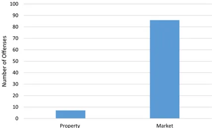
Figures 1 and 2 illustrate the distribution of our main variables. Note the difference in the monthly frequency of offending between property offenses and market offenses (7.07 vs. 85.92). However, the total monthly illegal earnings do not differ much between property and market offenses ($10,973 vs. $9,551), which makes the criminal effi-ciency between property and market offenses also starkly different ($1,552 vs. $111, respectively). 0 10 20 30 40 50 60 70 80 90 100 Property Market Number of Offense s
Fig. 1 Monthly frequency of offending
$0 $2,000 $4,000 $6,000 $8,000 $10,000 $12,000 Property Market
Monthly Illegal Earnings Criminal Efficiency
Time Varying Control Variables
To further account for unobserved heterogeneity, we control for a number of time varying covariates.
Legal Job Having a legal job is hypothesized to be inversely related to engaging income generating crimes (Sampson and Laub 1993). We include a dichotomous indicator if the respondent reported having a legal job during the month. Participants reported being employed approximately one third of the months in the window period.
Informal Job Informal or undeclared work can provide an alternative source of income that can be earned through income generating crimes (Nguyen et al. 2020). After report-ing the details of his legitimate work, the respondent was asked similar questions about his legitimate but undeclared employment. Overall, participants reported being employed informally about one third of the months in the window period.
Days Incarcerated To account for time that the respondent was free in the community to engage in crime, we control for the number of days a respondent was incarcerated each month. Respondents were asked about the months he was incarcerated. Offenders who engaged in property crimes reported being incarcerated on average 0.77 days each month, whereas those who engaged in market crimes reported being incarcerated 0.45 days each month during the window period.
Days Hospitalized In addition to being incapacitated by incarceration, the frequency of offending could be impacted by hospitalization. We control for the number of days a respondent was in the hospital each month to account for time that the respondent was free in the community to engage in crime. The respondent was asked if he was hospitalized dur-ing the window period. If he answered in the affirmative, he was asked which month(s) he was hospitalized and for how many days. Those who reported property crimes were hos-pitalized on average 0.16 days a month, whereas market offenders were hoshos-pitalized only 0.06 days on average a month.
Specialized in Property Crimes Specialization in the legal labor market is often asso-ciated with higher legal wages (Becker and Murphy 1992). Similarly, scholars have found that specialization in offense types is related to a higher illegal earnings premium (Loughran et al. 2013). Each respondent examined his monthly calendar to identify the months in which he participated in each of the crime types. For months that he reported participation in only property crimes, he was coded as being specialized in property crime. In 58% of the months, the respondents reported engaging in only property crimes.7
Specialized in Market Crimes Similarly, for the months that a respondent reported engaging in only market crimes, he was coded as being specialized in market crimes (75% of months).
On average, our respondents were 30 years old and had engaged in their first crime at age 15. Respondents were also serving an average sentence length of 22 months. Only 20% obtained a high school diploma or higher. Property offenders reported similar percep-tions of success with legal employment and criminal activities, whereas market offenders reported higher perceptions of success with criminal activities compared to legal employ-ment (Table 1).
7 This measure is similar to other studies that group together offense types as a measure of specialization
Results
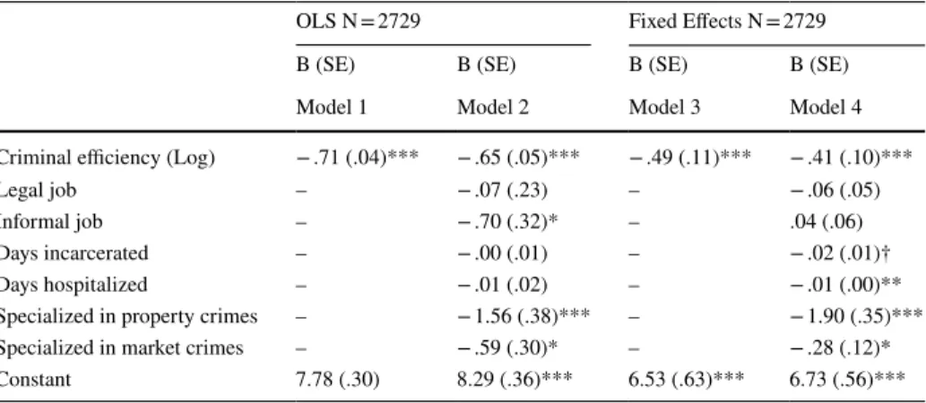
Table 2 reports model estimates for all crime types using the Quebec data. For each of the models, the unit of observation is person-month and standard errors are clustered at the
Table 1 Description of quebec sample
*Time stable measures are not used in fixed effects models
All crimes Property crimes Market crimes N = 2729 (152 people) N = 1174 (97 people) N = 2018 (105 people)
Mean (SD) Mean (SD) Mean (SD)
Time varying
Legal job .33 (–) .32 (–) .32 (–)
Informal job .21 (–) .22 (–) .17 (–)
Days incarcerated .47 (3.11) .77 (4.12) .45 (3.13)
Days hospitalized .11 (1.56) .16 (2.03) .06 (.98)
Specialized in property crimes .25 (–) .58 (–) –
Specialized in market crimes .55 (–) – .75 (–)
Time stable*
Age 31.20 (8.65) 30.05 (7.73) 31.38 (9.09)
Age first crime 15.12 (93) 14.36 (5.17) 15.41 (7.27)
Age first earned illegal income 18.51 (5.38) 17.66 (4.71) 18.75 (5.30) Length of current sentence
(months) 22.11 (29.09) 23.07 (21.71) 20.90 (30.62)
Number of children .73 (1.11) .74 (1.08) .66 (1.12)
High school diploma .19 (–) .21 (–) .19 (–)
Perceived success in legal work 1.68 (.93) 1.73 (.88) 1.65 (.90) Perceived success in crime 1.96 (1.03) 1.75 (.95) 2.10 (1.45) Annual legal income to desist (Log) 10.92 (.85) 10.96 (.88) 10.91 (.88)
Table 2 Panel models predicting illegal labor supply—all crimes (Robust Standard Errors)
† p < .10, *p < .05, **p < .01, ***p ≤ .001
OLS N = 2729 Fixed Effects N = 2729
B (SE) B (SE) B (SE) B (SE)
Model 1 Model 2 Model 3 Model 4
Criminal efficiency (Log) − .71 (.04)*** − .65 (.05)*** − .49 (.11)*** − .41 (.10)***
Legal job – − .07 (.23) – − .06 (.05)
Informal job – − .70 (.32)* – .04 (.06)
Days incarcerated – − .00 (.01) – − .02 (.01)†
Days hospitalized – − .01 (.02) – − .01 (.00)**
Specialized in property crimes – − 1.56 (.38)*** – − 1.90 (.35)***
Specialized in market crimes – − .59 (.30)* – − .28 (.12)*
individual level. In each case, the log–log specification allows us to directly interpret the coefficient on criminal efficiency as traditional elasticity, which can be interpreted as the % change in frequency/ % change in efficiency rate. Model 1 reports the elasticity esti-mated using traditional ordinary least squares (OLS). Model 2 reports the OLS estimates using additional controls. Models 3 and 4 display the results using individual fixed effects, the latter also including additional time-varying controls. The estimated elasticities range from − 0.71 (Model 1) to − 0.41 (Model 4) and in each case are statistically significant at α = 0.001. Moreover, in each case, a 95% confidence interval for the elasticity estimate would not include 1.
There are two important implications of these estimates. First, the negative elasticity implies that an increase in the criminal efficiency is associated with a decrease in over-all offending frequency. Second, the estimate is less than 1 (in terms of absolute value) implies that the frequency is inelastic, that is, the percentage change in frequency tends to be smaller than the proportion change in wage rate.
Interestingly, in the months that respondents do not specialize in property or market offenses, they offend less frequently, although this effect is stronger among property offend-ing. What this tells us is that, during the months that respondents only engage in prop-erty crime, frequency of offending is reduced by 190% (p < 0.001), whereas, in the months when respondents only engage in market offenses, offending frequency is only reduced by 28% (p < 0.05). There were no crime suppression effects of legal or informal work.
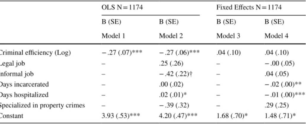
Table 3 reports analog models considering only property crimes, both in terms of fre-quency and criminal efficiency. While the OLS estimates of the supply elasticity are neg-ative and significant, the magnitudes of the estimates are much smaller than the overall estimates reported in Table 2. Moreover, elasticities become essentially zero (0.04) when including individual fixed effects. Days incarcerated (β = − 0.02, p < 0.01) and days hospi-talized (β = − 0.01, p < 0.001) significantly reduce the frequency of offending among prop-erty offenders in our fixed effects model. However, having a legal or informal job was not related to the frequency of offending.
Table 4 reports analog models for market crimes. The estimated elasticities are again negative and generally slightly larger in magnitude than the overall estimates in Table 2, ranging from − 0.76 in the OLS models to − 0.50 in the fixed effects estimates. In each case, the estimates are statistically significant at α = 0.05. Again, these estimates suggest
Table 3 Panel models predicting illegal labor supply—property crimes (Robust Standard Errors)
† p < .10, *p < .05, **p < .01, ***p ≤ .001
OLS N = 1174 Fixed Effects N = 1174
B (SE) B (SE) B (SE) B (SE)
Model 1 Model 2 Model 3 Model 4
Criminal efficiency (Log) − .27 (.07)*** − .27 (.06)*** .04 (.10) .04 (.10)
Legal job – .25 (.26) – − .00 (.05)
Informal job – − .42 (.22)† – .04 (.05)
Days incarcerated – .00 (.02) – − .02 (.00)**
Days hospitalized – .02 (.01)* – − .01 (.00)***
Specialized in property crimes – − .39 (.32) – .29 (.25)
that the supply for market-based crimes is largely inelastic. The number of days incarcer-ated is also inversely relincarcer-ated to frequency of offending (β = − 0.02, p < 0.001). Like prop-erty offenders, legal employment and informal employment are not significant among mar-ket offenders.
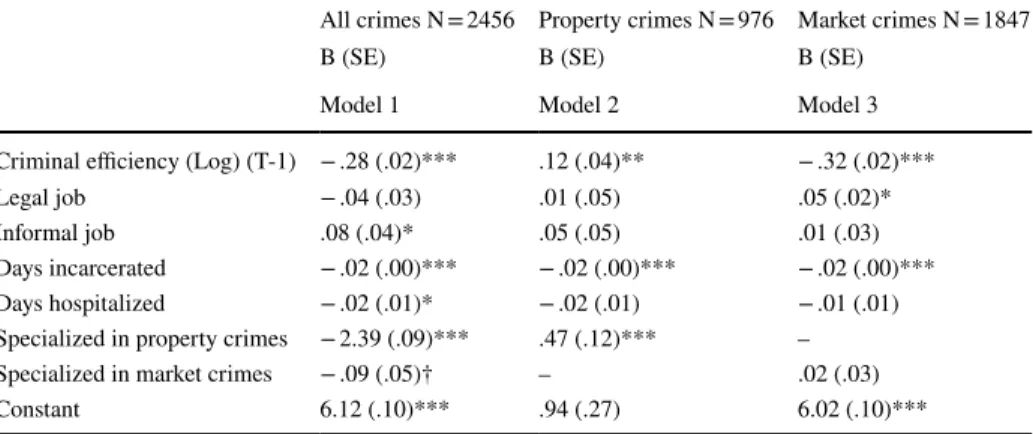
We also conducted fixed effects analyses where we lagged the criminal efficiency by one month and results are similar to the ones presented in the main tables (“Appendix A”).
Supplemental Analysis
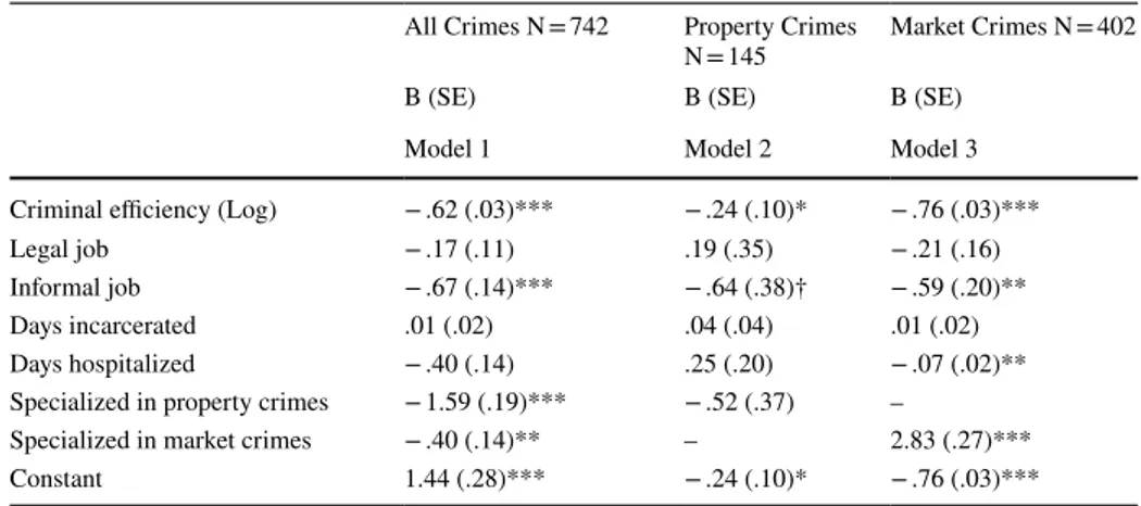
We consider the issue of individuals who report zero crime (and hence, zero earnings) in a given period. In such periods, there are two issues: the value of the dependent variable (fre-quency) and the value of the key independent variable (earnings/crime). The former, in which the individual chooses to commit zero crimes in a given period, can be treated as merely cen-sored at zero, and more importantly, observable (i.e., zero crime committed is a legitimate value). The latter quantity however, cannot be thought of as zero but rather unobservable due to truncation—i.e., there is some expectation of illegal wage ‘offer’ (higher than zero) that a potential offender has in mind when they are making their choice, but it is not high enough to induce them to act.8 How to deal with this issue is less straightforward, so we address it in two ways in supplemental analysis. First, Table 5 reports our results of first-difference analysis, which only includes observations with two adjacent illegal earnings periods. The first differ-ence results show how changes in frequency are changing in periods in which criminal effi-ciency are also changing (Table 5). Second, we conducted analysis which retains these period-specific zero observations but use an estimate of the wage rate based on cumulative efficiency (Table 6). In this case, we assume that an offender has an expectation of an illegal wage ‘offer’ based on their cumulative prior history of offending and earnings. The results of both sup-plemental analyses are consistent with our main findings, except for one main difference. The
Table 4 Panel models predicting illegal labor supply—market crimes (Robust Standard Errors)
† p < .10, *p < .05, **p < .01, ***p ≤ .001
OLS N = 2018 Fixed Effects N = 2018
B (SE) B (SE) B (SE) B (SE)
Model 1 Model 2 Model 3 Model 4
Criminal efficiency (Log) − .76 (.05)*** − .76 (.05)*** − .50 (.19)* − .50 (.19)*
Legal job – − .16 (.27) – .05 (.05)
Informal job – − .86 (.42)* – − .03 (.06)
Days incarcerated – − .03 (.02) – − .02 (.00)***
Days hospitalized – − .02 (.03) – − .01 (.07)
Specialized in market crimes – .25 (.29) – − .01 (.07)
Constant 8.01 (.31)*** 8.01 (.37)*** 6.79 (.89)*** 6.79 (.91)***
8 In a traditional wage regression in which earnings (rate) was the dependent variable, these values can be
treated using a traditional selection correction model in which the model parameters are corrected to adjust for selection bias (see Loughran et al. 2013). However, given that in the present case the unobserved values are on the right-hand side as opposed to the left-hand side, such a correction is not applicable.
supply elasticity are negative and significant for both property and market offenses. We note two things which may help reconcile this inconsistency from the prior. First, though statisti-cally significant, the magnitude of the relationship for property offenses is still considerably smaller than for market offenses. Second, it is possible that the cumulative measure may in fact be conflating crime types, given the tendency of certain crime types to occur in tandem.
Sensitivity Analysis
As a sensitivity check, we replicated these findings using both the Pathways to Desistance (Pathways) and National Supported Work (NSW) samples. We use the additional data sets to examine if the relationship between our key measures (criminal efficiency and frequency
Table 5 First-difference models predicting illegal labor supply
† p < .10, *p < .05, **p < .01, ***p ≤ .001
All Crimes N = 742 Property Crimes
N = 145 Market Crimes N = 402
B (SE) B (SE) B (SE)
Model 1 Model 2 Model 3
Criminal efficiency (Log) − .62 (.03)*** − .24 (.10)* − .76 (.03)***
Legal job − .17 (.11) .19 (.35) − .21 (.16)
Informal job − .67 (.14)*** − .64 (.38)† − .59 (.20)**
Days incarcerated .01 (.02) .04 (.04) .01 (.02)
Days hospitalized − .40 (.14) .25 (.20) − .07 (.02)**
Specialized in property crimes − 1.59 (.19)*** − .52 (.37) –
Specialized in market crimes − .40 (.14)** – 2.83 (.27)***
Constant 1.44 (.28)*** − .24 (.10)* − .76 (.03)***
Table 6 fixed effects models predicting illegal labor supply—average cumulative criminal efficiency (Robust Standard Errors)
† p < .10, *p < .05, **p < .01, ***p ≤ .001
All crimes N = 2739 Property crimes N = 1183 Market crimes N = 2020
B (SE) B (SE) B (SE)
Model 1 Model 2 Model 3
Avg cumulative criminal
effi-ciency (Log) − .50 (.02)*** − .30 (.03)*** − .99 (.04)***
Legal job − .02 (.03) − .04 (.05) .06 (.03)*
Informal job .07 (.04)† .01 (.05) − .06 (.03)†
Days incarcerated − .02 (.00)*** − .02 (.00)*** − .02 (.00)***
Days hospitalized − .02 (.01)† − .01 (.01) − .01 (.01)
Specialized in property crimes − 2.47 (.09)*** .24 (.09)* –
Specialized in market crimes − .02 (.05) – .04 (.04)
of offending) can be observed in other samples. While there are important differences across the data sets, additional samples provide us more confidence in the nature of the relationship of interest.
The Pathways study is a longitudinal examination of the transition from adolescence to young adulthood in a sample of serious adolescent offenders. The adolescents were selected for the study after a review of court documents indicated that they had been found guilty of a serious offense, such as felony offenses (Schubert et al. 2004). Originally, 1354 participants were enrolled and were between the ages of 14 and 17 years at the time of committing the offense and followed for seven years. The current study uses interviews col-lected from the first to the sixth interviews, which are the six month follow-ups. Because we limited the eligible observations to the first six waves, and not all participants reported earning money through illegal activities. A total of 442 respondents reported 747 periods of illegal wages.
The National Supported Work (NSW) Demonstration project provided basic, transi-tional job opportunities to individuals who are traditransi-tionally difficult to employ: ex-offend-ers, former drug addicts, and school dropouts. The Supported Work Project ran from 1975 to 1978 with about approximately 5,000 eligible applicants randomly assigned either to experimental groups (offered a job in supported work) or to control groups. Individuals who were eligible for participation in the study were referred by an official agency, such as employment, criminal justice and drug programs. Unlike the Pathways sample, not all par-ticipants were engaged in offending. At the time of enrollment, each respondent was given a retrospective baseline interview, followed by up to four follow-up interviews scheduled at nine-month intervals.
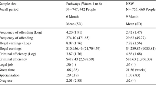
“Appendix B” displays information on the measures used from the respective studies. “Appendix C” displays the descriptive statistics for the two data sources. Table 7 reports fixed effects estimation of Eq. 2 using each sample both with and without the time-vary-ing controls in either case. In each of the data sets, the estimates of elasticity are remark-ably similar to those reported in the Quebec data (Table 2). For the Pathways analysis, the fixed effects estimate of elasticity is again negative (− 0.61), statistically significant, and less than 1 (a 95% confidence interval does not include 1). Similarly, for the NSW, the fixed effects estimate is negative (− 0.57), statistically significant, and less than 1 (a 95%
Table 7 Fixed effects models predicting illegal labor supply—pathways to desistance and national sup-ported work samples (Robust Standard Errors)
† p < .10, *p < .05, **p < .01, ***p ≤ .001
Sample size Pathways (Waves 1 to 6) NSW
N = 747; 442 People N = 755; 660 People
B (SE) B (SE) B (SE) B (SE)
Model 1 Model 2 Model 3 Model 4
Criminal efficiency (Log) − .61 (.05)*** − .57 (.05)*** − .57 (.05)*** − .59 (.06)***
Legal job – − .20 (.15) – − .12 (.20)
Street time – 1.30 (.27)*** – .02 (.01)**
Specialization – 2.34 (.44)*** – − .04 (.12)
Drug use – .09 (.03)** – .39 (.28)
confidence interval does not include 1). In each case the point estimates are negative and very similar in magnitude to the Quebec sample. Furthermore, in both cases the results again suggest that the relationship is largely inelastic.
There are several important similarities to the Quebec sample. The number of days on the street was positively related to offending frequency for both the Pathways (β = 1.30, p < 0.001) and the NSW (β = 0.02, p < 0.01) samples. Legal employment does not reduce frequency of offending in either the Pathways or NSW samples. Specialization (β = 2.34, p < 0.001) and drug use (β = 0.09, p < 0.01) are both positively related to frequency of offending, but only in the Pathways sample.
Despite the similarities, we caution the reader from drawing strong conclusions about directly comparing the three samples. To be clear, we understand that the Pathways and NSW samples present slightly different conditions, different populations, and different (i.e., coarser) temporal granularity and different controls. Respondents from the three sam-ples are involved with the criminal justice system and/or have limited legal opportunities. Results could differ with respondents that have not been involved in the criminal justice system.
Discussion
The present study was motivated by a fundamental yet overlooked question in crimino-logical theory: how sensitive are offenders to illegal monetary incentives? To answer our research question, we examined the relationship between monetary incentives and offend-ing by lookoffend-ing at within-individual change in offendoffend-ing frequency as a function of criminal efficiency, which we measure as the average pay-off per crime. Drawing on traditional eco-nomic concepts of labor supply, rational choice theory (Becker 1968); and prospect theory (Kahneman and Tversky 1979). We analyzed unique data from an incarcerated sample that offered detailed monthly measures on criminal efficiency, offending frequency, and life circumstances. Such data allowed us to assess within-individual changes in criminal effi-ciency and offending frequency. Our analyses led us to a finding of robust negative elastic-ity between criminal efficiency and offending frequency.
Overall, we found a robust negative relationship between criminal efficiency and offending frequency, which is contrary to a superficial reading of rational choice theory in which an increase in rewards would necessarily increase frequency. Our main find-ing tells us that, in the months that offenders have an average bigger pay-off per crime, they offended less frequently. We conjectured that this negative relationship could be explained by two mechanisms: an income effect and/or through reference dependence. The income effect highlights the trade-off between offending and leisure in that, as the pay-off per crime increases, an offender has more “purchasing power”. As discussed earlier, the negative relationship between criminal efficiency and offending frequency may suggest that, for some offenders, leisure and partying is a normal good. Offenders’ temporal horizons are likely short, as are the length of time over which an investment is made or held before it is liquidated. This lends some support to the low self-control premise that many offenders are unlikely to plan long term. This is also consistent with numerous qualitative studies that have elaborated on the indulgent lifestyles that many offenders live, even when they cannot afford to sustain it (e.g., Fleisher 1995; Hagan and McCarthy 1992; Jacobs and Wright 1999; Shover 1996). Offenders often spend
money conspicuously as to ‘‘create a look of cool transcendence’’ and show others that they are ‘‘members of the aristocracy of the streets’’ (Wright and Decker 1997, p. 40).
This same negative relationship, however, draws another interpretation when approached from prospect theory and one of its fundamental principles: reference dependence. Reference dependence suggests that an income target serves as a reference point. Not meeting the target would not then been seen as merely an absence in ille-gal income, but rather as a shortfall that is potentially treated as a relative loss (Heath et al. 1999). Consistent with prospect theory, this could then likely induce loss aversion, which would induce more risk-seeking behavior on the part of the individual to reach the target. At the same time and from the opposing trend, this would also reduce risk-seeking behavior in times when the reference point is met. Kőszegi and Rabin (2006,
2007) expand on Camerer et al.’s (1997) taxi driver research and find that, with day laborers, a worker is less likely to continue work if income earned thus far is unexpect-edly high, but more likely to show up as well as continue work if expected income is high. In this sense, and given the temporal setup of our data, we are unable to offer a conclusive argument that supports prospect theory. Future work on behavioral depar-tures from rational choice in offender decision-making is a rich area for research aimed at uncovering the more complex and detailed offender decision-making calculus.
One challenge that this study presents is the disentanglement of whether the negative elasticities are from the income effect or from reference dependence and income target-ing. Given that our sensitivity analyses show a similar negative relationship between criminal efficiency and offending frequency with larger time aggregations (one year for the Pathways sample and nine months for the NSW sample), it is more in line with an income effect. If we observed negative elasticity between criminal efficiency and offend-ing frequency at the monthly level, but not at larger time aggregations, we might have more support for reference dependence because larger time aggregations would allow offenders to inter-temporally substitute between months, offending more frequently in months with lower criminal efficiency and less in months with higher criminal effi-ciency (Camerer et al. 1997). One important avenue for future data collection efforts lies in questions designed to examine the underlying decision making processes related to earning and spending illegal income.
Offender lifestyles have been traditionally described as notoriously hedonistic, as evi-denced from past ethnographic work (Matza and Sykes 1961; Wright and Decker 1997) and emerging quantitative work (Felson et al. 2018). Our study contributes and expands the literature on criminal lifestyle by shifting the focus to offender decision making. An important implication of the often-observed hedonistic lifestyle of offenders is to under-stand how they spend money from various sources. According to Felson et al. (2018), “Offenders do not have enough income from legitimate sources to cover the expenses of such a hedonistic lifestyle, they engage in income producing crimes” (p. 3). In the cur-rent study, not only did we observe that the majority of offenders had legal employment during the months they engaged in crimes, we also observed that legal employment did not significantly reduce the frequency of offending. Future work should explore the con-cept of mental accounting among offenders. For example, there is substantial evidence that individuals conceptualize money from different sources in distinct ways, calling into question the fundamental economic principal of the fungibility of money (Thaler and Sefrin 1989). In other words, a dollar earned legally might be treated very different than a dollar earned illegally, specifically in how they are allocated for mental budgeting decisions (e.g., legal money might be set aside for rent, child care, while illegal money is used for partying, drugs, etc.).
According to Thaler (1999), money is labeled at three levels: expenditures are grouped into budgets (e.g., food, travel, household bills etc.); wealth is allocated into accounts (e.g., current, savings, pension, “petty cash”); and income is divided into categories (e.g., regular, windfall). In classic economics, it is assumed that money is fungible; money in one account is a perfect substitute for money in another; or regular income is function-ally equivalent to windfall income. However, there has been strong empirical evidence suggesting that individuals tend to separate consumption decisions into separate “mental accounts” (Thaler 1999), whereby income earned is not necessarily fungible across differ-ent budget categories (e.g., differ-entertainmdiffer-ent and food). Exploring the existence of differdiffer-ent mental accounts associated with multiple forms of income generating activities is impor-tant because how offenders think about money could influence their behavior towards money and approaches to generating it (Adams and Webley 2002). Importantly, the idea that individuals might have separate mental accounts for income earned legally, which is stable though limited, versus illegally, which is likely more ephemeral and transitory, is potentially a key driver of participation in either sector. The important point to retain here is that assessments of illegal earnings cannot be separated from more general earning pat-terns and it is precisely in this area where criminologists have limited themselves—they regularly decontextualize earning a living through crime and fail to situate their observa-tions and patterns in the wider repertoire of opobserva-tions for earning a living more generally.
Situating criminal earnings trends in the wider scope of earning options does indeed offer a greater range of explanations for specific and general crime patterns. Our key find-ing is that crime was inelastic to monetary returns. This suggests that dramatic shifts in incentives should not have a disproportionally large influence on offending frequency, con-trary to the findings by Freeman et al. (1999). This also suggests that, as with other types of inelastic labor, the supply of criminal offenses is driven largely internally and not neces-sarily easily accessible given severe price changes. Importantly, our findings are limited to conclusions about the intensive margin (frequency of offending), as opposed to the exten-sive margin (offending vs. not offending), in which others may be more induced to enter the market (who would otherwise not have previously done so) given a large change in earnings. Such an investigation is beyond the scope of the present analysis yet remains an important path for further investigation.
While we observed a robust negative elasticity between criminal efficiency and offend-ing frequency for market crimes, the relationship was less clear for property crimes. This suggests that the decision-making processes between market offenses and property offenses may differ. Given the higher frequency of market crimes, offenders have more variation in the number of market crimes s/he commits. Recall that, on average, respond-ents reported only 7 property crimes per month, whereas they reported 86 market offenses. The sheer opportunity and relative consensual nature of market crimes provides offend-ers with more opportunities to increase or decrease their offending frequency. Moreover, offenders engaged in market crimes are more reliant on the income generated from market crimes compared to offenders who engage in property crimes, which tend to be infrequent and episodic.
Interestingly, we did not find that having legal employment reduces offending frequency in any of our samples. Obtaining a good job is supposed to have many important implica-tions for offending. Theoretically, it is posited to be a key factor in building conventional social capital, providing a sense of accomplishment, organizing daily routines, serving as a source of informal social control, and facilitating other social roles that can inhibit crime, such as marriage (Sampson and Laub 1993; Uggen 2000). However, many individuals who engage in criminal activities also have a legal employment (Reuter et al. 1990). Fagan and
Freeman (1999) observed that, among disadvantaged young people in the 1980s, the divi-sion between legal and illegal ways of making money is not clear cut. Some persons com-mit crimes while legally employed, doubling up their legal and illegal activities. Thus, in line with the criminal career framework, legal employment may be one of the factors that is important for crime participation but not frequency of offending. Future research should include nuanced measures of both illegal and legal earnings to understand the dynamics between various forms of income generating activities.
Limitations
Our results do come with some caveats. First, while our within person design alleviates some sample selection bias, a currently emerging line of research is the examination of how different preferences can shift the supply curve for labor. Differences in attitudes (i.e., risk preferences, time horizons) across individuals and changes in attitudes within indi-viduals are associated with the supply of illegal labor. In such a case in which criminal earnings are determined endogenously, our estimation method may still result in some bias. More specifically, methods, such as the ones we employ in the current analysis, which are designed to eliminate bias due to selection are in fact not necessarily suitable to deal with bias which is the result of endogeneity (Nguyen and Loughran 2018), which among other things, precludes the use of sensitivity analyses designed to quantify the impact residual biases necessary to establish causality (e.g., VanderWeele and Ding 2017). As such, we are clear to avoid drawing any type of causal claims from the present analyses. That said, given the requisite statistical power necessary for more traditional methods to deal with endoge-neity (e.g., instrumental variables) to be employed and the fact that illegal earnings data is generally not observable in most large datasets, we believe our estimation approach serves as a point of departure into studying this question.
Second, our results are restricted to samples of offenders who reported earning money from crime in at least two recall periods. The Quebec study was designed to survey income generating offenders and therefore selection is less of an issue. To support this further, we conducted supplemental analyses using a first-difference estimator and using cumulative criminal efficiency. Sensitivity analyses with two additional data sets (Pathways and NSW) that differ in population and time period, were also conducted. Nonetheless, we heed cau-tion in generalizing our findings beyond the analytic samples used in this study. Future research should examine whether or not the same results hold among females or other income generating crime types, such as corporate crime.
The life history calendar method is one of the few methods that researchers have to measure longitudinal data. However, our results should be interpreted in light of the limita-tions of the method. van Gerwen et al. (2019) examined the accuracy of both the preva-lence and timing of specific life events among an incarcerated sample. They found that prevalence is relatively accurate compared to the timing of events. Morris and Slocum (2010) compared monthly level data, each study covering a three-year period, to official data on arrests and frequency of arrests. They similarly found the reports of prevalence and frequency of arrests were valid, while self-reported timing of arrests were less accurate. Policy Implications and Future Research
Although there is limited empirical evidence on the responsiveness of offenders to criminal efficiency, results from some studies demonstrate that offenders are sensitive to rewards
by examining the supply of crime to legal wages–that is, higher legal wages are associ-ated with a decline in crime. Using a sample of released federal prisoners from Maryland, Myers (1983) failed to detect strong traditional deterrent effects of certainty and sever-ity. Instead, results showed a strong reduction effect of higher legal wages on subsequent crime. Myers (1983) concluded that improving opportunities for legitimate employment is as an effective alternative to reducing crime as increasing punishment. Notably, Grogger (1998) examined the responsiveness of youth crime to labor market incentives. Grogger (1998) used the NLSY79 in a time allocation model of crime participation. In the model, consumers maximize their utility by choosing a combination of legal and illegal income generating activities. Grogger found that an increase in the legal wages would reduce the crime participation rate by 8%, suggesting that young men are responsive to wage incen-tives. Grogger (1998) noted, “consumers decide how much crime to commit and how much to work on the market as a function of their returns to crime…an hour spent committing crime causes no more disutility than an hour spent working” (p. 758). Recently, Agan and Makowsky (2018) analyzed administrative data and found that “the average minimum wage increase of $0.50 reduces the probability that men and women return to prison within 1 year by 2.8%”, supporting the argument that crime is a source of income.
Although a number of studies suggest that offenders are responsive to legal incentives (e.g., Agan and Makowsky, 2018; Grogger, 1998), if legal and illegal monies are not fungi-ble, minimum wage increases are likely to have limited impact on offending for some indi-viduals. The consumption choices and patterns of crime involved individuals is not well understood. The idea that offenders might internalize consumption using moneys from dif-ferent sources difdif-ferently and engage in mental accounting with illegal and informal funds has clear implications for conceptual and theoretical studies of offender decision-making (Loughran 2019; Pogarsky et al. 2018; Paternoster 2010). Moreover, it has potentially important implications for public policy and poverty and crime prevention interventions. For example, supported work and income maintenance programs are based on the idea of financial stability through legal channels will help aid transitions to crime cessation. Consumption of non-standard or non-necessity commodities such as luxury items, or more illicit things such as drug, alcohol or gambling might be driven by illegal incentives more heavily than commensurate legal means.
The empirical research of the responsivity of offenders to illegal incentives is in its nas-cent stages, even though there is a rich literature on the responsivity of offenders to the costs associated with offending behavior. It is only through fostering further research to explore the role of illegal incentives on behavior that we can begin to formulate clearer policy implications.
Appendix A
Appendix B
Pathways to Desistance and National Supported Work Measures Pathway Measures
Frequency of Offending Subjects reported the frequency in which they engaged in income-generating crime during the recall period. Income-generating crimes include shoplifting, buying/receiving/selling stolen property, using checks/credit cards illegally, stealing a car or motorcycle, selling marijuana, selling other drugs, stealing something worth more than $100, entering a building to steal, taking something by force using a weapon, and taking something by force with no weapon.
Illegal Earnings Participants were asked, “Have you made money in other ways over the past N months, including from activities that are illegal?” If the respondent answered in the affirmative, the interviewer asked a follow-up question: “You mentioned that you had made money during the past N months from ways besides working. Did you make any money during this month from activities that are illegal?” For each month in which subjects engaged in any illegal work, they were asked to specify the amount of money per week they earned from all illegal activities during that month.
Criminal Efficiency was measured as the average payoff per crime, calculated by dividing total illegal earnings by the total number of crimes committed each month in which offenders were active.
Legal Job The legal employment variable was derived from a life-event calendar, which recorded detailed information regarding the total number of weeks each subject spent in legitimate employment and under-the-table legal work. This information was then aggregated across each observation period. If the respondent reported any time in legitimate employment in the recall period, s/he was coded as being involved in legal work in the recall period.
Street Time Is the proportion of time the respondent was not in a secure facility. Table 8 Panel models predicting illegal labor supply—lagged criminal efficiency (Robust Standard Errors)
† p < .10, *p < .05, **p < .01, ***p ≤ .001
All crimes N = 2456 Property crimes N = 976 Market crimes N = 1847
B (SE) B (SE) B (SE)
Model 1 Model 2 Model 3
Criminal efficiency (Log) (T-1) − .28 (.02)*** .12 (.04)** − .32 (.02)***
Legal job − .04 (.03) .01 (.05) .05 (.02)*
Informal job .08 (.04)* .05 (.05) .01 (.03)
Days incarcerated − .02 (.00)*** − .02 (.00)*** − .02 (.00)***
Days hospitalized − .02 (.01)* − .02 (.01) − .01 (.01)
Specialized in property crimes − 2.39 (.09)*** .47 (.12)*** –
Specialized in market crimes − .09 (.05)† – .02 (.03)