2D/3D knowledge inference for intelligent access to enriched visual content

(1)

HAL Id: tel-00917972

https://tel.archives-ouvertes.fr/tel-00917972

Submitted on 12 Dec 2013

HAL is a multi-disciplinary open access archive for the deposit and dissemination of sci-entific research documents, whether they are pub-lished or not. The documents may come from teaching and research institutions in France or abroad, or from public or private research centers.

L’archive ouverte pluridisciplinaire HAL, est destinée au dépôt et à la diffusion de documents scientifiques de niveau recherche, publiés ou non, émanant des établissements d’enseignement et de recherche français ou étrangers, des laboratoires publics ou privés.

2D/3D knowledge inference for intelligent access to

enriched visual content

Raluca-Diana Sambra-Petre

To cite this version:

Raluca-Diana Sambra-Petre. 2D/3D knowledge inference for intelligent access to enriched vi-sual content. Other [cs.OH]. Institut National des Télécommunications, 2013. English. �NNT : 2013TELE0012�. �tel-00917972�

(2)

Spécialité: Informatique et Télécommunications

Ecole doctorale: Informatique, Télécommunications et Electronique de Paris

Présentée par

Raluca-Diana ŞAMBRA-PETRE

Pour obtenir le grade de DOCTEUR DE TELECOM SUDPARIS

MODELISATION ET INFERENCE 2D/3D DE CONNAISSANCES POUR

L'ACCES INTELLIGENT AUX CONTENUS VISUELS ENRICHIS

Soutenue le 18 Juin 2013 à Paris

devant le jury composé de :

Président de jury: Madame le Maître de Conférences, HDR Catherine ACHARD Rapporteur: Monsieur le Professeur Marc ANTONINI Rapporteur: Monsieur le Professeur Constantin VERTAN Examinateur: Monsieur le Professeur Miroslaw BOBER Examinateur: Monsieur le Docteur Olivier MARTINOT Directeur de thèse: Monsieur le Professeur Titus ZAHARIA

Thèse n°: 2013TELE0012

(3)

(4)

2D/3D KNOWLEDGE INFERENCE

(5)

(6)

ACKNOWLEDGMENT

First, I would like to express my gratitude to my thesis supervisor, Professor Titus Zaharia, for his guidance throughout my thesis and for all fruitful discussions that we had. His wide knowledge and his logical way of thinking have been of great value for me. I would also like to thank him for being attentive towards me and providing me with invaluable encouragements.

I would like to address my special thanks to the members of my Ph.D. defense committee. To Professor Catherine Achard, from Pierre and Marie Curie University, President of this Jury, I would like to express all my thanks for her interest in my research work.

I would also like to express all my gratitude to Professors Marc Antonini from Nice Sophia Antipolis University and to Professor Constantin Vertan, from POLITECHNICA University of Bucharest, for accepting the hard task of being reviewers. Their reviews, comments and fruitful suggestions helped me to improve the manuscript and to give it its final shape.

A special thank to Miroslaw Bober from University of Surrey who provided encouraging and very constructive feedback.

I am very thankful to Mr. Olivier Martinot, Research Department Director at Alcatel-Lucent Bell Labs, for our collaboration and for accepting to be member of the examination jury.

I would also like to mention that this work has been performed within the framework of the UBIMEDIA Research Lab, established between Institut Mines-Télécom and Alcatel-Lucent Bell-Labs.

My gratitude goes also toward my colleagues and friends, from ARTEMIS and beyond, which supported me during all these years. To Madame Evelyne Tarroni I would like to thank for her help and patience in efficiently solving all necessary administrative problems.

I also like to thank my colleagues Ruxandra and Bogdan for sharing with me much more than just an office. One of the best things that my PhD experience brought me is the beautiful friendship with Afef. I thank her for always lifting my spirit when I felt down and overwhelmed with problems.

A very special thank to my dear friend Alina, which has always been available to hear about my difficulties and who offered me unconditional support.

I will never thank enough my husband, Andrei, who gave me strength and motivation to overcome all difficulties. He offered me moral support, as well as priceless technical and linguistic advices and helped me to improve my work and my experience.

(7)

2D/3DKNOWLEDGE INFERENCE FOR INTELLIGENT ACCESS TO ENRICHED VISUAL CONTENT

I would finally like to thank my family for their continuous love and support. A special thank you goes to my grandfather who, at the age of 81 years, tried to understand my doctoral work and to help me with his ideas.

(8)

LIST OF FIGURES

Figure I.1 Different views of a 3D object representing a bicycle. ... 2

Figure II.1 Main stages of 2D/3D Indexing. ... 7

Figure II.2 Affine transformations of a 3D Model. ... 8

Figure II.3 Sensibility to minor modification of bounding box-based centring. ... 9

Figure II.4 Example of principal axes determined with weighted PCA. ... 12

Figure II.5 Example of similar models presenting differently detected principal axes. ... 12

Figure II.6 3D-to-2D projection. ... 15

Figure II.7 Different representations of a 2D shape. ... 18

Figure II.8 Selection of the principal and secondary axes. ... 21

Figure II.9 MCC-based representation. ... 23

Figure II.10 Silhouette intersection. ... 24

Figure II.11 Principle of the PPD approach. ... 25

Figure II.12 PCA miss-alignment. ... 26

Figure II.13 Dissimilar objects presenting similar views after scale normalization... 27

Figure III.1 The 3D model retrieval scheme. ... 37

Figure III.2 PCA3 viewing angle selection strategy. ... 39

Figure III.3 Secondary views used by the PCA7 viewing angle selection strategy. ... 39

Figure III.4 DODECA viewing angle selection strategy. ... 40

Figure III.5 DDPCA viewing angle selection strategy. ... 40

Figure III.6 Octahedron-based viewing angle selection strategy. ... 41

Figure III.7 Icosahedron-based viewing angle selection strategy. ... 41

Figure III.8 RV10 views selection strategy. ... 43

Figure III.9 The Angular Radial Transform (ART) basis functions. ... 45

Figure III.10 The Hough Transform. ... 46

Figure III.11 Examples of Hough Transforms. ... 46

Figure III.12 Zernike basis functions. ... 47

Figure III.13 Contour Scale Space. ... 48

Figure III.14 Angular Histogram — humanoid. ... 50

(13)

VI

Figure III.16 3D models matching. ... 51

Figure III.17 3D models matching with the Minimum strategy. ... 52

Figure III.18 Sample models from the MPEG7 3D dataset. ... 54

Figure III.19 Sample models from the PSB 3D dataset. ... 54

Figure III.20 Intra and inter class variability. ... 56

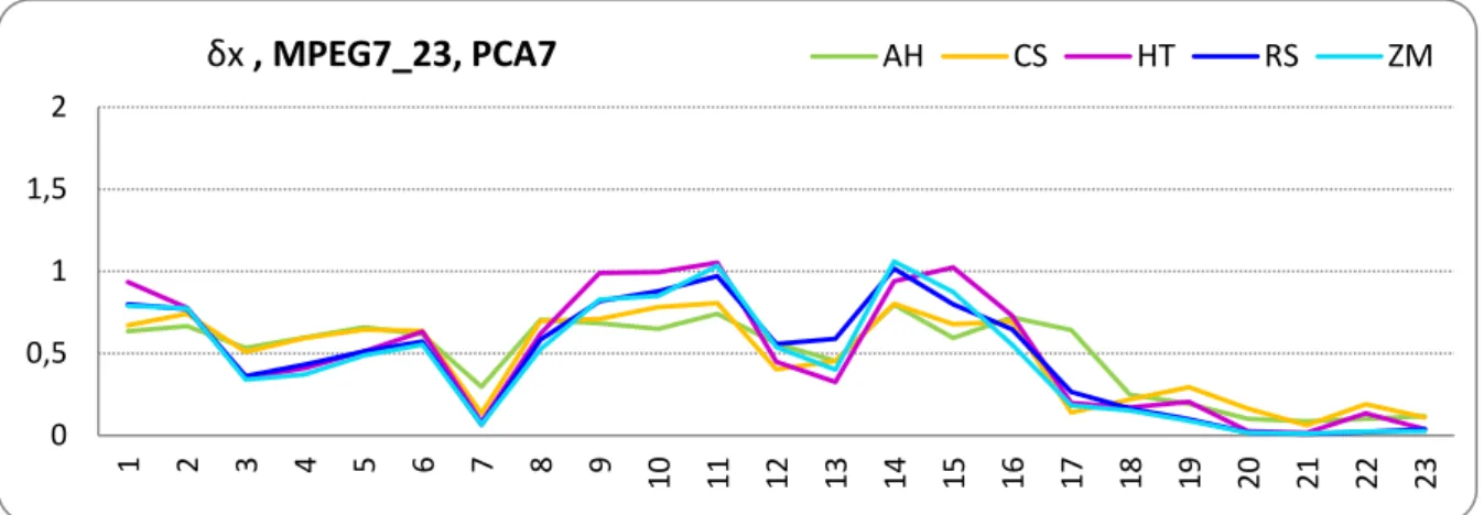
Figure III.21 MPEG7_23 database: Intra-class variability with PCA7 strategy. ... 62

Figure III.22 PSB_53 database: Intra-class variability with PCA7 strategy. ... 62

Figure III.23 PSB_161 database: Intra-class variability with PCA7 strategy. ... 62

Figure III.24 Separability / inter-class variability – MPEG7_23 database. ... 63

Figure III.25 Separability / inter-class variability – PSB_53 database. ... 64

Figure III.26 Separability / inter-class variability – PSB_161 database. ... 65

Figure III.27 Example of airplane retrieval result. ... 67

Figure III.28 The Precision-Recall curve associated with the example in Figure III.27. ... 67

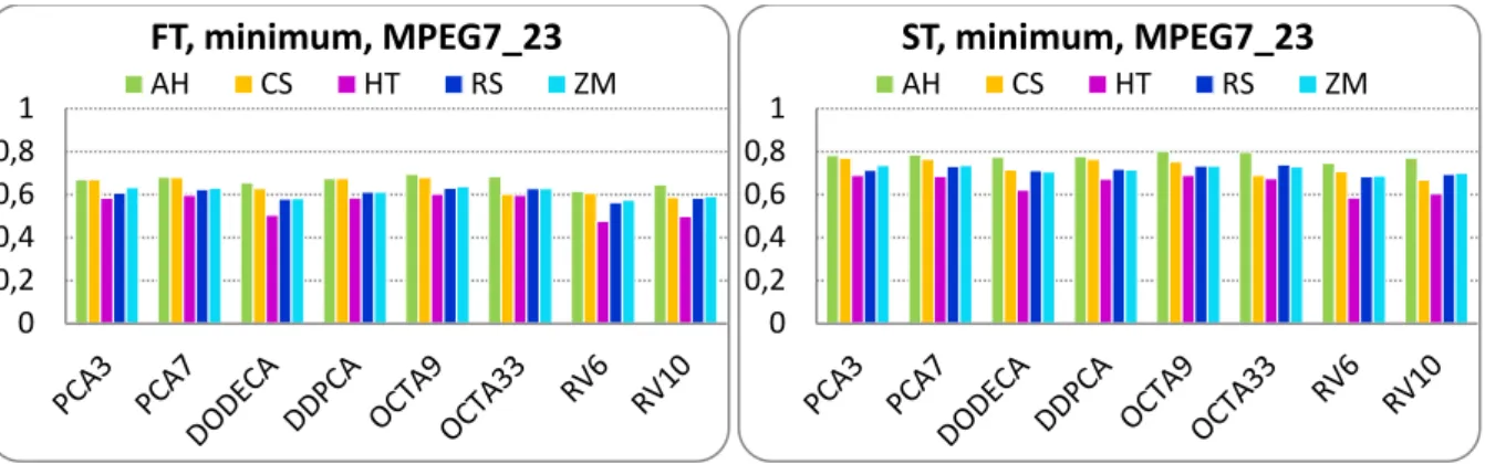
Figure III.29 MPEG7_23 database: FT and ST score, minimum matching strategy. ... 70

Figure III.30 MPEG7_23 database: FT and ST score, diagonal matching strategy. ... 70

Figure III.31 PSB_53 database: FT and ST score, minimum matching strategy. ... 70

Figure III.32 PSB_53 database: FT and ST score, diagonal matching strategy. ... 70

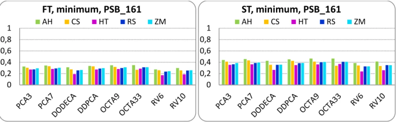
Figure III.33 PSB_161 database: FT and ST score, minimum matching strategy. ... 71

Figure III.34 PSB_161 database: FT and ST score, diagonal matching strategy. ... 71

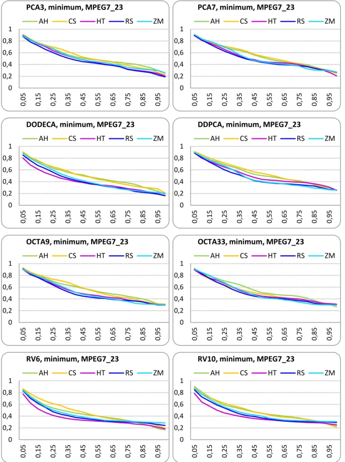
Figure III.35 MPEG7_23 database: Precision-Recall curves, minimum matching strategy. ... 72

Figure III.36 MPEG7_23 database: Precision-Recall curves, diagonal matching strategy. ... 73

Figure III.37 PSB_53 database: Precision-Recall curves, minimum matching strategy. ... 74

Figure III.38 PSB_53 database: Precision-Recall curves, diagonal matching strategy. ... 75

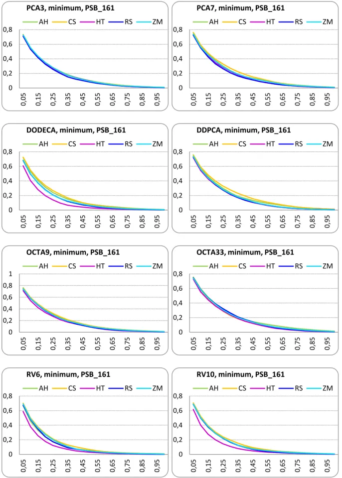
Figure III.39 PSB_161 database: Precision-Recall curves, minimum matching strategy. ... 76

Figure III.40 PSB_161 database: Precision-Recall curves, diagonal matching strategy. ... 77

Figure IV.1 Still object recognition framework. ... 90

Figure IV.2 Video object recognition framework. ... 92

Figure IV.3 Still object dataset. ... 94

Figure IV.4 Sample frames from VOV test set and the corresponding segmented objects. ... 95

Figure IV.5 The 3D models selected to generate the synthetic image dataset. ... 96

Figure IV.6 Example of recognition rate computation. ... 98

Figure IV.7 SOI database: RR(1) and RR(3) scores ... 100

(14)

LIST OF FIGURES

Figure IV.9 SOI database: RR(1), RR(3) and RR(10) scores ... 100

Figure IV.10 SOSy database: RR(1) and RR(3) scores ... 101

Figure IV.11 SOSy database: RR(1) and RR(3) scores ... 101

Figure IV.12 SOSy database: RR(1), RR(3) and RR(10) scores... 101

Figure IV.13 SOV database: RR(1) and RR(3) scores ... 102

Figure IV.14 SOV database: RR(1) and RR(3) scores ... 102

Figure IV.15 SOV database: RR(1),RR(3)and RR(10) scores ... 102

Figure IV.16 SOI database: RR(3) scores per category ... 104

Figure IV.19 SOSy database: RR(3) scores per category ... 105

Figure IV.22 SOV database: RR(3) scores per category ... 106

Figure IV.25 SOI database – combined descriptors: RR(1) and RR(3) scores ... 107

Figure IV.26 SOI database – combined descriptors: RR(1) and RR(3) scores ... 107

Figure IV.27 SOI database – combined descriptors: RR(1), RR(3) and RR(10) scores ... 107

Figure IV.28 SOSy database – combined descriptors: RR(1) and RR(3) scores ... 108

Figure IV.29 SOSy database – combined descriptors: RR(1) and RR(3) scores ... 108

Figure IV.30 SOSy database – combined descriptors: RR(1), RR(3) and RR(10) scores ... 108

Figure IV.31 SOV database – combined descriptors: RR(1) and RR(3) scores ... 109

Figure IV.32 SOV database – combined descriptors: RR(1) and RR(3) scores ... 109

Figure IV.33 SOV database – combined descriptors: RR(1), RR(3) and RR(10) scores ... 109

Figure IV.34 VOV database: RR(1) and RR(3) scores ... 111

Figure IV.35 VOV database: RR(1) and RR(3) scores ... 111

Figure IV.36 VOV database: RR(1),RR(3)and RR(10) scores ... 111

Figure IV.37 VOV database – combined descriptors: RR(1) and RR(3) scores ... 112

Figure IV.38 VOV database – combined descriptors: RR(1) and RR(3) scores ... 112

Figure IV.39 VOV database – combined descriptors: RR(1), RR(3) and RR(10) scores ... 112

Figure IV.40 VOSy database: RR(1) and RR(3) scores obtained with DODECA ... 113

(15)

VIII

Figure IV.42 VOSy database: RR(1),RR(3)and RR(10) scores obtained with DODECA ... 113

Figure V.1 Various scribbles encountered in the literature. ... 117

Figure V.2 Graph representation exploited in the Graph Cut approach. ... 118

Figure V.3 Star-shape condition: a. example of star-shaped object. ... 120

Figure V.4 Example of GMM-based segmentation. ... 124

Figure V.5 The segmentation process. ... 125

Figure V.6 Example of segmentation. ... 126

Figure V.7 Example of segmentation. ... 127

Figure V.8 Compression influence on the segmentation result. ... 128

Figure V.9 Background likelihood map for the 50% compressed image illustrated in Figure V.8. ... 129

Figure V.10 Segmentation results for uncompressed and compressed images ... 129

Figure V.11 Example of elongated Gaussian distribution. ... 129

Figure V.12 Example of 1D Gaussian distributions. ... 130

Figure V.13 Compression block artefacts for a soft toy image. ... 131

Figure V.14 Example of Gaussian distribution in Luv colour space. ... 132

Figure V.15 Compression artefacts reduction with modified GMM. ... 133

Figure V.16 Example of segmented object. ... 135

Figure V.20 The influence of JPEG compression. ... 138

Figure VI.1. DIANA platform architecture. ... 145

Figure VI.2 The Web server. ... 146

Figure VI.3 DIANA Web platform: the 3D models databases page. ... 147

Figure VI.4 DIANA Web platform: the 3D – 3D searching page. ... 148

Figure VI.5 DIANA Web platform: the 2D – 3D searching page. ... 149

Figure VI.6 DIANA Web platform: the segmentation and classification page. ... 150

Figure A.1 Mesh representation. ... 157

(16)

LIST OF TABLES

Table II.1 Overview of 2D/3D indexing approaches ... 34

Table III.1 Overview of adopted 2D shape descriptors ... 53

Table III.2 Normalization reference ... 57

Table III.3 MPEG7_23 database: inter-class variability and separability ... 60

Table III.4 PSB_53 database: inter-class variability and separability ... 60

Table III.5 PSB_161 database: inter-class variability and separability ... 60

Table III.6 MPEG7_23 database: intra-class variability ... 61

Table III.7 PSB_53 database: intra-class variability ... 61

Table III.8 PSB_161 database: intra-class variability ... 61

Table III.9 MPEG7_23 database: FT and ST score with minimum matching strategy ... 78

Table III.10 MPEG7_23 database: FT and ST score with diagonal matching strategy ... 78

Table III.11 PSB_53 database: FT and ST score with minimum matching strategy ... 78

Table III.12 PSB_53 database: FT and ST score with diagonal matching strategy ... 78

Table III.13 PSB_161 database: FT and ST score with minimum matching strategy ... 79

Table III.14 PSB_161 database: FT and ST score with diagonal matching strategy ... 79

Table V.1 Overlap score on original and compressed images. ... 136

Table A.1 List of categories included in the MPEG7_23 database ... 159

Table A.2 List of categories included in the PSB_53 database ... 159

Table A.3 List of categories included in the PSB_161 database ... 160

Table A.4 List of SOI categories tested with MPEG7_23 database ... 162

Table A.5 List of SOI categories with PSB-53 and PSB_161_23 databases ... 162

Table A.6 List of SOV and VOV categories ... 162

Table A.7 List of SOSy and VOSy categories ... 162

Table A.8 SOI database: Recognition rates obtained with the help of MPEG7_23 models. ... 163

Table A.9 SOI database: Recognition rates obtained with the help of PSB_53 models. ... 163

Table A.10 SOI database: Recognition rates obtained with the help of PSB_161 models. ... 164

Table A.11 SOSy database: Recognition rates obtained with the help of MPEG7_23 models. ... 165

Table A.12 SOSy database: Recognition rates obtained with the help of PSB_53 models. ... 165

(17)

X

Table A.14 SOV database: Recognition rates obtained with the help of MPEG7_23 models. ... 167

Table A.15 SOV database: Recognition rates obtained with the help of PSB_53 models. ... 167

Table A.16 SOV database: Recognition rates obtained with the help of PSB_161 models. ... 168

Table A.17 VOV database: Recognition rates obtained with the help of MPEG7_23 models. ... 169

Table A.18 VOV database: Recognition rates obtained with the help of PSB_53 models. ... 169

Table A.19 VOV database: Recognition rates obtained with the help of PSB_161 models. ... 170

Table A.20 VOSy database: Recognition rates obtained with the help of MPEG7_23 models. ... 171

Table A.21 VOSy database: Recognition rates obtained with the help of PSB_53 models. ... 171

(18)

I. INTRODUCTION

Graphics hardware and software development domains have seen a vast expansion in the last decades. Due to the spectacular evolution in digital technologies, the amount of multimedia content (i.e., still images, videos, 2D/3D graphics…) available today is continuously increasing. Within this context, disposing of powerful search and retrieval methods becomes a key issue for intelligent and efficient access to audio-video material.

When large databases of multimedia content are involved, user access to specific material of interest is not possible without efficient search engines.

Multimedia retrieval tools may be divided into two main families: concept-based and content-based techniques. In the first case, some metadata, such as keywords and tags, are associated to the multimedia data and the retrieval is performed starting from textual indices. However, the linguistic barriers represent an important drawback of such approaches. Also, a prior, manual annotation is required, which is a tedious and highly subjective process.

In contrast, in content-based retrieval the search process analyzes the actual content of the data (e.g., colour, shape, texture, and motion feature for describing the visual appearance…). By using computer vision algorithms, the salient features of the multimedia content are revealed and transformed into numerical representations, so-called descriptors. Such descriptors allow an objective comparison of different audio-video materials, making it possible to perform similarity retrieval of multimedia data.

Moreover, such objective descriptors can be used for classification purposes. More precisely, they can be employed to evaluate the similarity between multimedia materials. Thus, if we dispose of categorized content, we can analyse its similarity with respect to any unknown multimedia material in order to automatically assign one of the existing classes to the new material.

A large number of existing methods uses prior knowledge in order to accomplish this kind of objective. Such approaches generally exploit machine learning (ML) techniques. They automatically learn to recognize complex structures based on sets of both positive and negative

(19)

2

examples. ML techniques involve two main stages. First, some characteristic features are extracted starting from a set of examples involved in the training phase. Then, these features are used in order to recognize new cases. Such methods should be able to generalize the features of a given class while ensuring the accuracy of the recognition process.

However, when a large number of categories is involved, the number of recognition criteria (and implicitly the number of exploited features) increases and thus the computational complexity may become intractable. In addition, in order to allow generalization, a large variety of examples should be used in the training set. Moreover, a given object may present highly different appearances due to pose variation. Thus, for effective ML-based 2D object classification purposes, the training set should include not only a variety of examples but also different instances of the same object, corresponding to different poses (Figure I.1).

Figure I.1 Different views of a 3D object representing a bicycle.

The first (profile) and the last (front) views are completely different in terms of 2D shape, but can be related if the 3D model is available.

This thesis specifically addresses the issue of still image and video object classification. In our work, we propose to overcome the limitation of existing ML approaches by exploiting the information contained in categorized 3D model repositories. In order to enable the transfer of semantic labels from 3D models to 2D objects, shape-based 2D/3D indexing methods are employed. The 2D/3D description (also known as view-based description) consists of characterizing a 3D model through a set of 2D views. Further, the shape features are extracted and used in the recognition process. The choice of using only the shape information is motivated by the fact that the shape is a feature shared by all object within a class, compared to the colour or the texture which may change from one object to another. The availability of 3D models (involved in the recognition process) is not an issue because nowadays a large amount of 3D object collections

(20)

INTRODUCTION

can be found on the internet. Moreover, these repositories are already classified, which represents an important advantage within the proposed framework.

The main purpose of this thesis is the exploitation and evaluation of 2D/3D indexing techniques within the context of 3D model retrieval as well as for 2D or 2D + t object classification purposes.

Chapter II introduces the main 2D/3D indexing techniques. The background definitions and terminologies are here recalled and several important issues related to the view-based description process are discussed. A review of the state of the art methods is also presented.

Chapter III presents the 2D/3D indexing approaches adopted in our work. We notably introduce here a new clustering-based method for adaptive selection of representative views and a novel contour-based descriptor, so-called Angular Histogram (AH). The 3D model repositories exploited in our work are also presented and an objective intra and inter class variability analysis is proposed. The performances of the various 2D shape descriptors and viewing angle strategies retained are experimentally evaluated within a 3D model retrieval framework.

The object classification issue is addressed in the fourth chapter. The view-based indexing methods presented previously are here employed to allow semantic inference between 3D and 2D content. The underlying principle consists of exploiting the a priori knowledge contained in classified 3D models and to transfer it, with the help of view-based indexing, to unknown 2D objects. Such methods can be applied to both still objects (SO, i.e., objects extracted from still images) and video objects (VO, i.e., objects extracted from videos and composed of several instances). We propose here a classification framework which ensures fast computation and allows combining several indexing methods. A main contribution of our work, compared to state of the art 3D model-based classification approaches, is the capacity to deal with a large number of semantic classes (up to 161 categories). In order to experimentally evaluate the performances of the recognition framework, we have created several test sets, including objects extracted from real and synthetic images and videos.

In order to allow integrating the proposed 2D object recognition framework in real applications, we have also developed a segmentation approach, designed to assist the user to extract an object of interest from an image. The proposed method, presented in chapter V, adopts the scribble-based segmentation paradigm. The user interaction consists of specifying a set of lines, corresponding to both foreground and background scribbles. The segmentation process is based on colour distributions, estimated with Gaussian Mixture Models (GMM). In order to overcome the compression artefacts that may appear, a modified GMM model is proposed. The experimental evaluation demonstrates the superiority of the modified GMM model which is able to appropriately take into account compression artefacts.

Finally, an important aspect in 2D/3D object retrieval and recognition is to dispose of appropriate user interfaces. The proposed DIANA (Digital Image Analysis aNd Annotation) system is a Web platform integrating the various developments proposed in this thesis. Chapter VI presents the main tools and functionalities proposed by the DIANA platform.

Chapter VII concludes the manuscript, highlights the main contributions proposed in this work and opens some perspectives of future research.

(21)

(22)

II. 2D/3D INDEXING

Abstract. This chapter introduces the view-based 3D model indexing. The principle of the 2D/3D

description methods is first presented. The background definitions and terminologies are briefly recalled and several important issues related to 2D/3D indexing are discussed.

In the second part of the chapter we review the state of the art methods. We propose a classification of the various approaches, based on the viewing angles selection strategy employed. We conclude with an analysis of the advantages and limitations related to each family of 2D/3D indexing methods.

Keywords: shape descriptor; projection strategy; 3D meshes; 2D/3D indexing; similarity

(23)

(24)

2D/3DINDEXING

The concept of 2D/3D indexing refers to a class of 3D model description methods. Their particularity is that a 3D model is not directly characterized in the 3D space, but instead through a set of 2D projection views, which provide the 2D appearance of the model from different perspectives/angles of view.

The underlying principle of 2D/3D indexing approaches is based on the following observation: two similar 3D models should present similar views when projected in 2D images from similar perspectives (e.g., frontal projection, profile projection…). Such a strategy allows comparing two different 3D models through their corresponding 2D views. In addition, and more interestingly, such view-based approaches make it possible to compare not only 3D models, but also to match 3D models with 2D objects.

This chapter first presents the principle of the 2D/3D indexing paradigm, with the necessary theoretical background and main concepts involved. The state of the art methods are then described and analyzed, and the main methodological challenges that still need to be solved are identified.

II.1. T

HEORETICAL

B

ACKGROUND

The 2D/3D indexing includes several stages (Figure II.1). First, a pre-processing pose normalization step is required in order to ensure a canonical representation of the 3D mesh geometry. Next, the model is projected into 2D, resulting in a set of views. Finally, each view is described with the help of a 2D shape descriptor.

a. b. c. d.

Figure II.1 Main stages of 2D/3D Indexing.

a.&b. Pose normalization; c. 3D-to-2D projection; d. 2D shape description.

When analyzing this process, some fundamental questions rise up: how many projection views are needed to obtain an accurate representation of the considered 3D shape? Which are the angles of view of the model that optimally represent its shape? Which shape descriptors are suited for this purpose?

The various solutions proposed in the state of the art for each stage involved are detailed in the following sections.

(25)

8

II.1.1. Pre-processing: normalization and invariance issues

Existing 3D models are most often specified with arbitrary orientations, positions and scales in the 3D virtual space. In our case, we have considered exclusively 3D models represented as 3D mesh models (cf. Annexe A1). Thus, the model geometry is specified by the set of 3D position of the mesh vertices, in a given 3D coordinate system. However, not all shape descriptors are intrinsically invariant to geometric transforms. Therefore, in order to ensure at least an extrinsic invariant behaviour, it is necessary to apply some position/pose/size normalization.

Thus, the objective is to prepare the 3D model for 2D/3D indexing by offering invariance with respect to similarity transforms (i.e., translation, rotation, isotropic scaling and combinations of them  Figure II.2). After the normalization process, similar models should present similar size, orientation and position in the 3D virtual space. In addition, the normalization process should be robust to small, local deformations of the model.

The normalization process includes the following three steps:

 Centring: consists of positioning the 3D model with respect to the origin of the coordinate system and ensures invariance to translation.

 Alignment: consists of orienting the 3D model in the virtual space, which ensures invariance to rotation.

 Scaling: consists of resizing the object in order to ensure scale invariance.

The following sections detail the main pose normalization techniques encountered in the literature.

II.1.1.1. Model centring

The centring consists in displacing the 3D model such that its "centre" coincides with the origin of the coordinate system. There exists several ways to define the centre of a 3D model.

II.1.1.1.1. The centre of the bounding box

A first approach [Paquet00] defines the centre of a 3D model as the centre CBB of its

corresponding bounding box and is defined as:

a. b. c.

Figure II.2 Affine transformations of a 3D Model. a. translation; b. rotation; c. scaling.

(26)

2D/3DINDEXING

(II.1)

where:

 xmin, xmax, ymin, ymax, zmin, zmax respectively denote the minimum and maximum coordinate

values of the 3D mesh vertices, along the x, y and z axes.

Let us observe that the centre of a 3D model’s bounding box is not invariant with respect to rotations. Therefore, such a bounding box centring approach should be applied after the alignment phase.

The main drawback of the bounding box-based centring is the sensibility to minor shape modifications, as illustrated in Figure II.3. Here, two 3D models of tanks are presented, which correspond to the same real-life objects. The difference between them concerns the position of the tank machine gun, which points horizontally in Figure II.3a and vertically in Figure II.3b. As a result, the corresponding bounding boxes are significantly different and centring approach will lead to an erroneous result. Let us note that this situation is often appearing in practice, in the case of articulated shapes (i.e., shapes composed of multiple parts that can independently exhibit rigid motion).

a. b.

Figure II.3 Sensibility to minor modification of bounding box-based centring.

II.1.1.1.2. The gravity centre

The gravity centre (G) is also known as centre of mass or centre of inertia and represents the barycentre of the 3D mesh M, defined as described in the following equation:

(II.2)

where:

 NT is the number of the mesh triangles;

 Ai_{represents the area of the i}th _triangle;

 gi

x,y,z are the coordinates of the gravity centre of the ith triangular face.

As the entire surface of the 3D model is taken into consideration when computing , the

barycentre method is less sensitive to minor modification of the shape than the bounding box approach. Thus, in our work we have considered that the centre of a 3D model is given by the barycentre, computed as described in Equation II.2.

(27)

10

II.1.1.2. Pose alignment

The pose alignment phase aims at ensuring rotation invariance. For this purpose, an object-dependent, orthogonal 3D coordinate system needs to be constructed first. An orthogonal transform is then applied in order to transform the initial coordinate system in an object-dependent one.

The most commonly employed approach is to consider the system defined by the three axes

of inertia of the 3D mesh. The axes of inertia, also known as principal axes, are obtained with the

help of a Principle Component Analysis (PCA) approach [Mather04], [Schwengerdt97]. The PCA technique involves a mathematical procedure that transforms a set of possibly correlated variables (e.g., the coordinates of the 3D model's vertices) into a set of uncorrelated variables, called principal components.

Various types of information and data can be used for 3D model alignment, including vertex coordinates and normal vectors.

In the PCA framework, such data are considered as realizations of a 3D random vector. A

m  3 matrix, denoted by X, is constructed; it stores on each row a realization Xt_{of the random}

vector:

(II.3)

Most often, the number of observations m is equal to the number of mesh vertices V and the observations Xt_{represent the x, y and z coordinate values of the mesh vertices.}

The (3 × 3) covariance matrix Σ of X is then computed as described by the following equations: (II.4) (II.5) with (II.6)

In Equation II.4, E [.] and (.) T_{respectively denote the statistical expectation and the matrix}

transpose operators.

By definition, the covariance matrix is symmetric and positive definite. Thus, it can be diagonalized with the help of an orthogonal transform constructed as a matrix V with the eigenvectors as columns. In addition, the corresponding eigenvalues are real and positive numbers, which provide a measure of extent of the object along each eigen-direction. More precisely, the following equation is satisfied:

(28)

2D/3DINDEXING

_(II.7)

where D is a diagonal matrix storing the eigenvalues of Σ.

The eigenvectors Vi that compose the matrix V are also called principal axes or axes of

inertia. The planes defined by each couple of eigenvectors are referred to as principal planes. Finally, the 3D object pose alignment is accomplished by applying the following transformation:

(II.8)

Let us note that depending on the space where the PCA is performed, two families of PCA methods can be distinguished: discrete and continuous PCA. The discrete case corresponds to the matrix formulation presented here above, where a finite set of observation is employed. Matrix X can store the coordinates of the vertices, the coordinates of the face gravity centres or the normal vectors associated with polygonal face. The main limitation of such approaches is the dependence on the distribution of the vertices, in the case where the mesh vertices are irregularly distributed. In order to overcome this drawback, [Paquet00] propose to weight the contribution of each gravity centre by the area of the corresponding triangular face.

In the case of continuous PCA (CPCA) approach [Vranic01], the analysis is performed in the infinite-dimensional space of the mesh surface σ. Here, the covariance matrix is defined as the matrix of second order surface moments.

(II.9)

where:

 A is the total area of the 3D mesh surface;

 p = (xp,yp,zp) is a point on the surface of the 3D mesh;

 mijk is the moment of order , defined as:

(II.10)

Compared to discrete PCA approaches, CPCA is more accurate, at the price of an increased computational complexity [Chaouch09].

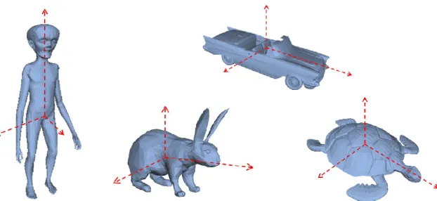
In our work we have adopted the weighted PCA methods [Paquet00] which ensures good results with a limited computational complexity. Figure II.4 presents some examples of 3D models and corresponding principal axes for various shapes, obtained with the weighted PCA approach. We observe that in such cases, the PCA alignment corresponds to intuitive notions, such as frontal, profile and bottom views.

Whatever the approach considered, the main drawback of the PCA-based alignment is related to its incapacity of dealing with miss-alignment problems, in the case where different axes of inertia are computed for similar 3D models [Zaharia01, Tangelder04].

(29)

12 Three miss-alignment situations may appear:

 The two sets of principal axes have significantly different orientations. This problem, illustrated in Figure II.5 a and b, is a stability issue, which arises in the case where some object details affect the symmetry of the objects.

 The same orientations are detected for both models, but the order of the principal components is not the same. Let us note that the ordering of the eigenvectors in the construction of the transform matrix V in Equation II.7 is important, since different orders lead to completely different transforms. Most of the time, such an ordering is performed with respect to the values of the corresponding eigenvalues. However, such a mechanism can lead to erroneous alignments, as illustrated in Figure II.5 a and c.

 The principal components have the same directions for both models, but different orientations: solely the PCA cannot uniquely determine the orientation of the eigenvectors, but gives only their direction. This ambiguity leads to miss-alignments in the case of non-symmetric objects, as illustrated in Figure II.5 a and d.

a. b. c. d.

Figure II.5 Example of similar models presenting differently detected principal axes. a. the reference model; b. the principal axes has a different orientation w.r.t the model's geometry; c. the principal axes have different order compared to those of the reference model; d. the principal

axes have different directions than those of the reference model. Figure II.4 Example of principal axes determined with weighted PCA.

(30)

2D/3DINDEXING

Another alignment approach is proposed in [Papadakis08]. Let M be a mesh, A its total surface area, and α, β and γ rotation angles around the Ox, Oy and Oz axes, respectively. Let

M(α,β,γ) denote the rotated model. The aim of the so-called rectilinearity-based alignment is to

determine the set of angles (α,β,γ) maximizing the fallowing ratio: _(II.11) where:

 , and represent the areas of the

projections on the (xy), (yz) and (zx) planes of the rotated model.

Compared to discrete PCA, the rectilinearity-based alignment present higher computational complexity.

II.1.1.3. Model scaling

The objective of the model scaling stage is to determine an intrinsic scale for each 3D model in order to normalize the object in size and achieve representation invariance.

II.1.1.3.1. Bounding sphere approach

In order to determine the bounding sphere, the farthest vertex from the centre of the object is first determined and the corresponding distance (dmax) is computed. The maximum distance dmax

represents the radius of the bounding sphere. The normalization is accomplished by resizing the model to the unit sphere.

This normalization technique is invariant to rotation and translation. However, such a naive approach is highly sensitive to minor changes of the 3D mesh or to articulated shape (cf. Section II.1.1.1.1) which can modify the value of dmax.

In order to overcome such a limitation, different techniques exploit the eigenvalues computed in PCA in order to statistically determine the intrinsic scale.

II.1.1.3.2. Eigenvalue-based normalization

In [Elad02], authors propose to rescale the model such as the largest eigenvalue (D11)

becomes equal to 1.

Such an approach presents the same drawback as PCA: in some cases, for two similar models, the principal axes can have different directions and orientations. Thus, the corresponding eigenvalues are different and the scale normalization is not the same for both models.

In order to overcome this drawback, in [Zaharia02] the authors propose to consider the three eigenvalues D11, D22, D33 (cf. Equation II.7). The object is resized such as the expression

(31)

14

II.1.1.3.3. Distance to surface

In [Vranic04], authors propose to determine the intrinsic scale of the model based on the mean distance between the object surface σ and the principal planes.

(II.12)

where:

 represent the mean distance from the model surface to (yz), (xz) respectively (xy) planes:

_(II.13)

where:

 p=(px,py,pz) is a point on the surface σ of the model;

 G=(Gx,Gy,Gz) is the centre of the 3D model;

 A is the area of the 3D model surface;

Normalization is accomplished by resizing the model such that the computed distance

becomes equal to a given value.

Another distance-based method [Vranic04] proposes to define the intrinsic scale based on the mean distance from the centre C of the model to its surface σ.

_(II.14)

Here again, the 3D model is resized such as the distance becomes equal to a given value.

Compared to other scale normalization techniques, the distance to surface-based approach is more robust to small shape deformations but computationally more complex.

In our work, we have adopted the eigenvalues-based scaling due to its robustness and low computational complexity required within our framework (the eigenvalues are already computed in the alignment phase).

Once normalization in orientation, size and position is completed, the 2D views of the 3D model can be acquired, with the help of a 3D-to-2D projection mechanism, as described in the following section.

(32)

2D/3DINDEXING II.1.2. 3D-to-2D projection

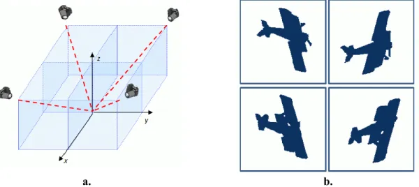
The projection of the 3D model into 2D images represents a key phase in 2D/3D indexing process. The mesh model M is projected and rendered in 2D from NP different viewing angles

(i.e., positions of a virtual camera in the 3D space) (Figure II.6 a), resulting in a set of NP

projections, denoted by Pi (M), with i=1..NP.

The projection may be a binary image (the silhouette of the object) or a gray level image representing the depth map (Figure II.6 b and c). However, only the silhouette representation allows matching between 2D and 3D content, as there is no depth information available in 2D images.

A viewing direction {ni} is associated to each viewing angle; it represents the direction of

the straight line that connects the position of the camera with the origin of the considered Cartesian system (which, after normalization, coincides with the centre of the 3D model).

When projecting a 3D model for 2D/3D indexing purpose, the key aspects that need to be considered concern the number of considered views and the specification of the viewing angles.

II.1.2.1. The number of views

The number of views (NP) defines how many views are generated for each object. A large

number of views ensures good description of the 3D model, which is suited for indexing and retrieval purposes. However, the associated computational aspects have to be taken into account. The time required for projection and descriptor extraction, as well as memory/storage requirements, are proportional to the number of views. Therefore, a “good” balance has to be ensured between the level of detail of the 2D/3D representation and the computational costs involved.

a. b. c.

Figure II.6 3D-to-2D projection.

(33)

16

II.1.2.2. The viewing angles

The viewing angles (directions) {ni} define the perspectives used to generate the set of

views. Obviously, there is an infinity of potential viewing angles. However, some views are more salient than other. In addition, there exists couples of very similar views. For 2D/3D indexing purposes, only the shape information is exploited. Under the assumption of a parallel projection model, the silhouettes obtained from opposite perspectives (e.g., front and back, left and right, up and down) represent mirror reflections of each other. In order to avoid representation redundancy, solely a demi-space around the model should be considered for specifying the views.

There exist three main families of viewing angle selection strategies. A first and largely popular family makes the assumption that the most salient views correspond to the projection onto the principal planes. Therefore, the viewing directions correspond to the principal axes of the model. Throughout this work, this class of approaches will be referred to as PCA-based viewing angle selection.

The second family of approaches considers that there are no preferential viewing directions. Therefore, the viewing angles are distributed as evenly as possible around the object. Most often, in this case the camera repartition is obtained using the vertices of a regular polyhedron (e.g., octahedron, dodecahedron...).

Finally, the third class of viewing angles selection strategy attempts an intelligent selection of the views. First, a large number of evenly distributed views is generated. Next, the similarity between views is analyzed and a subset of representative views is selected to represent the 3D model. In order to measure the similarity between two views, each view is characterized with the help of shape descriptors. A discussion on descriptor extraction and similarity measurement can be found in the following sections.

The main disadvantage of the representative views strategies is the computational costs which includes the achievement and description of a large number of views as well as the high number of pairwise comparison between couples of views needed. A second drawback is related to the intrinsic nature of such strategies: two different 3D models will be described by completely different, object-dependent views. How is it possible, in this case, to specify a matching strategy that can be exploited for 3D model retrieval purposes?

Whatever the viewing angle selection strategy adopted, the 2D shape descriptors involved for describing the resulting silhouettes strongly influence the discriminative power of the representation. Descriptor-related aspects are discussed in the following section.

II.1.3. 2D shape descriptors

Descriptors are mathematical representations of the salient features of the multimedia content which allow an objective and quantitative comparison between various objects. For 2D-3D matching purposes the shape attribute represents the most popular feature considered.

Let us first recall the various criteria enounced in the literature that a shape descriptor should satisfy [Zaharia04], [Tangelder04]:

(34)

2D/3DINDEXING

 Scope: the descriptor should be able to characterize any kind of shape.

 Uniqueness: a given shape is described by only one descriptor and a given descriptor corresponds to a single shape.

 Efficiency: for a large database, the system should be able to quickly describe models and to perform a fast retrieval. Therefore, rapidity and low complexity of the feature extraction is necessary. Some descriptors allow early rejection of non-similar models based on a subset of features. This ability is useful for speeding up the matching process.

 Robustness: the descriptor should be almost insensitive to noise and to small extra features.  Sensitivity: a descriptor should present the capacity to describe and take into account even

fine details of the shape.

 Discrimination power: the descriptor should be able to capture the properties that best discriminate the shape.

 Multiresolution support: the descriptor should not depend on the resolution of the shape.  Ability to perform partial matching: such a feature is useful in the case of incomplete

shapes, such when a part of the object is invisible (for example, in the case of occluded objects).

 Geometric and topologic invariance: the description of a given object should not depend on the scale, orientation or position that it has in the image.

 Agreement with the human perception: it is important that the similarities given by a descriptor correspond to the human perception.

 Ability to match articulated objects: a descriptor should extract similar features for different instances of an articulated object.

 The storage size of the descriptor: an important property especially in the case of big databases where a large number of descriptors must be stored.

Such criteria are taken into account in various manners by the different approaches of the state of the art, which can be categorized within three main families of 2D shape descriptors:

 Region shape descriptors: in this case, the input information to be described represents the support region of the 2D shape (Figure II.7b).

 Contour shape descriptors: solely the external contour information is retained (Figure II.7c). Consequently, the principal limitation of such approaches concerns the limited area of applicability, since shapes with more complex topologies (e.g., holes, multiple connected components...) cannot be accurately described.

 Graph-based descriptors: the principle consists of setting-up a part-based representation, achieved with the help of a graph or a multi-level graph (Figure II.7d). In some cases, the nodes of the graph may store attributes of the corresponding region of the 2D object. The advantage of such elaborate representations is the possibility to represent accurately complex shape and, in particular, articulated shapes. However, specifying fast similarity measures for graph-based representations, which is mandatory for indexing and retrieval applications, is still an open issue of research.

(35)

18

a. b. c. d.

Figure II.7 Different representations of a 2D shape.

a. The 3D model; b. Region support; c. Contour representation; d. Graph representation. The various 2D shape descriptors of the state of the art are presented and discussed in Section II.2.

Whatever the type of descriptor considered, it is of outmost importance to define appropriate similarity measures between them.

II.1.4. Similarity measurement

The similarity measurement employs the mathematical representation of the shape features (i.e., the descriptor) in order to associate a quantitative appreciation to the similarity between shapes.

Depending on the shape descriptor considered, one of the following similarity measurement methods can be used:

 Distance (metric)-based methods, suitable for feature vector representation and supposed to compute metrics such as the Euclidian distance.

 Graph matching methods, specifically adapted for graph-based representations.

II.1.4.1. Distance metric-based method

The distance metric measures the dissimilarity between two vectors. A small value denotes that the two vectors are very similar while higher values correspond to dissimilar vectors. In order to ensure good similarity estimation, a distance metric must satisfy several properties, recalled here below.

II.1.4.1.1. Distance metric properties

Let X, Y, Z be three vectors in a n-dimensional space and a function defined as (II.15)

Then, the function d is a distance if it satisfies the following properties:

 Identity: ; the distance between two identical vectors should be equal to zero.  Positivity: ; the distance between two different vectors should always have a

(36)

2D/3DINDEXING

 Symmetry: ; the distance from X to Y should be equal to the distance from Y to X.

 Triangle inequality: ; the distance from X to Z is at most as large as the sum of the distances from X to Y and from Y to Z.

 Transformation invariance: , where g is a transformation in a given group. In the particular case of shape description, the group of similarity transforms is most often considered. This means that the distance between two shapes is independent of their position, size or orientation.

Various distance metrics can be used. They are recalled in the following section.

II.1.4.1.2. Distance metrics

Let and be two points in the space. Several

metrics are defined in order to measure the distance between X and Y:

Minkowski distance of order p:

(II.16)

Manhattan distance (L1 norm):

(II.17)

Euclidean distance (L2 norm):

(II.18)

Weighted Euclidean distance:

(II.19)

where wi represents the weight of each component of the n-dimensional space.

Hausdorff distance:

(II.20)

where:

(37)

20

 represents the shortest distance between X and a given element y of Y and is

given by the closest element x of X to y;

 represents the longest distance from Y to X;

Let us note that the Hausdorff distance [Atallah83, Dubuisson94] is very sensitive to noise, since even a single outlier can affect its value.

Earth mover’s distance (EMD): represents the minimum effort required to transform the

distribution of X into the distribution of Y. The distributions are interpreted as mounds of sand and the distance represents the cost of turning one mound into the other, knowing that moving an amount ε of earth from a point i to a point j takes effort (with d a distance metric such as the Euclidian distance) [Rubner00].

Kullback-Leibler divergence (KLD): is not a real distance because it is a non-symmetric

measure. X and Y are considered as two distributions having the associated codes CX, respectively

CY. KLD measures the number of extra bits required to code samples of X using CY rather than

using CX.

II.1.4.2. Graph matching methods

If the shape of 2D objects is represented by a graph, then a graph matching procedure is necessary in order to compare the two shapes.

The aim of a graph matching method is to determine the best correspondence between the two graph representations. The resemblance level between graphs is given by a function which measures the similarity between couples of corresponding vertices and edges. The graph matching approach can also be seen as an energy minimization algorithm [Bengoetxea02].

There exist two classes of matching methods. When the two graphs have the same size (i.e., the same number of vertices) an isomorphic mapping can be found between them. This family is called exact matching. On the contrary, when the two graphs have different sizes, the one-to-one correspondence becomes impossible. This case is referred to as inexact matching.

The combinatorial nature of the graph matching approaches leads to high computational complexity, which most often is NP-complete [Garey79, Conte04].

Let us now detail how the various aspects presented above are taken into account in the literature.

II.2. S

TATE OF THE

A

RT

The literature presents a large variety of 2D/3D indexing methods, mainly developed for 3D model retrieval purpose. Since the choice of viewing directions is a fundamental issue for successful 2D/3D description, we have categorized various families of approaches with respect to the viewing angle selection strategy (cf. Section II.1.2.2). The classification adopted in our work includes:

(38)

2D/3DINDEXING

 Methods using PCA-based projections make the underlying assumption that the views corresponding to the projection on the principal planes present higher relevance than other views.

 Methods using evenly distributed viewing angles offer the same importance to all the views around the model.

 Methods using representative views include a clever selection of the views used in the 2D/3D description.

Let us begin our analysis with the PCA-based projection approaches.

II.2.1. Methods using PCA-based projection

As a representative of the 2D/3D shape-based retrieval approaches, let us first mention the

MultiView description scheme (DS) proposed by MPEG-7 standard [Bober02, Manjunath02,

ISO/IEC02].

The pre-processing stage involves translation and scaling, the 3D object being transformed such that its gravity centre coincides with the coordinate system origin and fits the unit sphere. The rotation invariance is achieved by applying a principal component analysis (cf. Section II.1.1.2).

Three views are generated by projecting the 3D model onto the principal planes (Figure II.8a). Four secondary views can be added in order to ensure better description. The secondary viewing directions correspond to the diagonal of the octants defined by the principal planes (Figure II.8b). Figure II.8c illustrates the repartition of the seven cameras and the corresponding viewing directions.

a. b. c.

Figure II.8 Selection of the principal and secondary axes.

a. The three principal viewing directions which corresponds to the first three principal axes; b. the secondary viewing angles; c. the seven cameras reparation;

(39)

22

Concerning the shape descriptors, let us first mention the MPEG-7 framework [ISO/IEC02], where two different MPEG-7 2D shape descriptors, the Contour Shape (CS) and the Region

Shape (RS), have been considered.

In the case of the RS descriptor, the object's support function is decomposed within a base of Angular Radial Transform (ART) functions [Kim99]. Thus, the image is be represented as a weighted sum of ART coefficients. In order to achieve rotation invariance, solely the absolute values of the coefficients are used. The similarity measure simply consists of L1 distances

between ART coefficients. The 2D-ART is invariant under similarity transforms, and it is suitable for meshes of arbitrary topologies, which can present holes or multiple connected components under the projection operator. A more detailed presentation of the RS descriptor can be found in Section III.2.2.1.

The second 2D shape descriptor promoted within the MPEG-7 DS is Contour Shape (CS), which employs the Contour Scale Space (CSS) representation[Mokhtarian92]. More restrictive, the MPEG-7 CS descriptor assumes that the shape of the object can be described by a unique, closed contour. The descriptor is obtained by successively convolving an arc-length parametric representation of the curve with a Gaussian kernel. The curvature peaks are thus robustly determined in a multi-scale analysis process and serve to characterize the contour shape, with their value and corresponding position (expressed as curvilinear abscise).The associated similarity measure between two contours in CSS representation is the EMD [Rubner00]. A more detailed discussion on the CS descriptor is presented in Section III.2.2.4.

Whatever the 2D shape descriptor considered, when comparing two 3D models MA and MB,

a distance value eij is obtained for each pair of views Pi(MA) – Pj(MB). An error matrix E=(eij) is

thus computed. The global similarity measure between the two models is then defined as:

(II.21)

where





represents the set of all possible permutations between the columns of matrix E;  p is a permutation in



;

 p(E) represents the permuted version of matrix E.

Let us note that such a similarity measure is highly expensive since the number of possible permutations is NP!, where NP is the number of projections. In practice, such a similarity measure

can be applied only for a reduced number of views and becomes computationally un-tractable when the number of views increases (3!=6, 7!=5040).

In [Mahmoudi02], authors re-visit the MPEG-7 CSS representation. Here, the contour of each projection image is represented in CSS and decomposed into a set of segments called tokens,

i.e., sets of 2D points delimited by two inflexion points. The tokens are then clustered and

hierarchically organized in a M-Tree structure [Ciaccia97]. This organization allows to considerably decrease the computation time, as proved by their experimental evaluation. To compare two tokens, a sum of geodesic distances between points is computed. The obtained descriptor is intrinsically invariant to similarity transforms.

(40)

2D/3DINDEXING

The M-Tree-based CSS algorithm was further developed in [Mahmoudi07], where a Bayesian voting procedure is employed. To each part pi of the contour is associated a posterior

probability Pr(pi|Pj(M)) that reflects what is the chance to have a given view Pj(M) in the image,

knowing the presence of the part pi. Based on the posterior probability, a rank R(Q, Pj(M)) can be

associated to query image Q with respect to a given view Pj(M). The rank denotes the similarity

between the query and the view and is calculated as the sum of posterior probabilities Pr(pi|Pj(M))

for all parts pi composing the contour of Q. A notable consequence of the Bayesian voting

procedure is that it allows partial matching. Also, the experimental evaluation presented in [Mahmoudi07] has shown that the Bayesian approach increases the performance of the M-Tree-based CSS algorithm.

Another method based on multi-scale shape representation is proposed in [Napoléon08]. Here, the authors employ a 2D/3D approach based on the MCC (Multi-scale

Convexity/Concavity) representation introduced in [Adamek04]. The 3D object is scaled with

respect to its bounding sphere and CPCA is applied in order to normalize the pose of the model. A number of three to nine silhouettes are then computed. The viewing directions used correspond to the three principal axes and to their six bisectors.

Each silhouette is further represented by its contour, normalized to sample points. As in the case of the CSS descriptor, a scale-space analysis is performed here. Each silhouette contour is successively convolved with Gaussian functions, with increasing kernel bandwidths σ (Figure II.9b). Then, the displacement of the position of sample u between two consecutive scale levels σi-1 and σi is computed. The MCC representation is a

100  10 matrix composed of the displacements of all 100 contour sample points for the 10 scale levels (Figure II.9c).

a. b. c.

Figure II.9 MCC-based representation.

a. the initial contour; b. the convolved contours; c. the MCC representation;

The similarity measure used to compare two MCC representations is given by the L1