HAL Id: hal-02087763
https://hal.inria.fr/hal-02087763
Submitted on 2 Apr 2019
HAL is a multi-disciplinary open access
archive for the deposit and dissemination of
sci-entific research documents, whether they are
pub-lished or not. The documents may come from
teaching and research institutions in France or
abroad, or from public or private research centers.
L’archive ouverte pluridisciplinaire HAL, est
destinée au dépôt et à la diffusion de documents
scientifiques de niveau recherche, publiés ou non,
émanant des établissements d’enseignement et de
recherche français ou étrangers, des laboratoires
publics ou privés.
Graph Data
Silviu Maniu, Pierre Senellart, Suraj Jog
To cite this version:
Silviu Maniu, Pierre Senellart, Suraj Jog. An Experimental Study of the Treewidth of Real-World
Graph Data. ICDT 2019 – 22nd International Conference on Database Theory, Mar 2019, Lisbon,
Portugal. pp.18, �10.4230/LIPIcs.ICDT.2019.12�. �hal-02087763�
Real-World Graph Data
Silviu Maniu
LRI, CNRS, Université Paris-Sud, Université Paris-Saclay, Orsay, France [email protected]
Pierre Senellart
DI ENS, ENS, CNRS, PSL University, Paris, France Inria Paris, France
LTCI, Télécom ParisTech, Paris, France [email protected]
Suraj Jog
University of Illinois at Urbana–Champaign, Urbana-Champaign, USA [email protected]
Abstract
Treewidth is a parameter that measures how tree-like a relational instance is, and whether it can reasonably be decomposed into a tree. Many computation tasks are known to be tractable on databases of small treewidth, but computing the treewidth of a given instance is intractable. This article is the first large-scale experimental study of treewidth and tree decompositions of real-world database instances (25 datasets from 8 different domains, with sizes ranging from a few thousand to a few million vertices). The goal is to determine which data, if any, can benefit of the wealth of algorithms for databases of small treewidth. For each dataset, we obtain upper and lower bound estimations of their treewidth, and study the properties of their tree decompositions. We show in particular that, even when treewidth is high, using partial tree decompositions can result in data structures that can assist algorithms.
2012 ACM Subject Classification Theory of computation → Logic and databases
Keywords and phrases Treewidth, Graph decompositions, Experiments, Query processing
Digital Object Identifier 10.4230/LIPIcs.ICDT.2019.12
Related Version An extended version of this paper is available at http://arxiv.org/abs/1901. 06862.
Acknowledgements We are grateful to Antoine Amarilli and Mikaël Monet for feedback on parts of this paper.
1
Introduction and Related Work
A number of data management tasks related to query evaluation are computationally intractable when rich query languages or complex tasks are involved, even when the query is assumed to be fixed (that is, when we consider data complexity [60]). For example:
query evaluation of Boolean monadic second-order (MSO) queries is hard for every level of the polynomial hierarchy [4];
unless P = NP, there is no polynomial-time enumeration or counting algorithm for first-order (FO) queries with free second-order variables [57, 29];
computing the probability of conjunctive queries (CQs) over tuple-independent databases, a very simple model of probabilistic databases, is #P-hard [25];
unless P = NP, there is no polynomial-time algorithm to construct a deterministic decomposable negation normal form (d-DNNF) representation of the Boolean provenance of some CQ [25, 40]; furthermore, there is no polynomial bound on the size of a structured d-DNNF representation of the Boolean provenance of unions of conjunctive queries with disequalities [11, Theorem 33].
Other problems yield complexity classes usually considered tractable, such as AC0 for
Boolean FO query evaluation [1], but may still result in impractical running times on large database instances.
To face this intractability and practical inefficiency, one possible approach has been to determine conditions on the structure of databases that ensure tractability, often through a series of algorithmic meta-theorems [44]. This has led, for instance, to the introduction of the notions of locally tree-decomposable structures for near-linear-time evaluation of Boolean FO queries [33], or to that of structures of bounded expansion for constant-delay enumeration of FO queries [41].
Treewidth. A particularly simple and widely used way to restrict database instances that
ensures a wide class of tractability results is to bound the treewidth of the instance (this is actually a special case of both notions of locally tree-decomposable and bounded expansion).
Treewidth [56] is a graph-theoretic parameter that characterizes how tree-like a graph, or
more generally a relational instance, is, and hence whether it can be reasonably transformed into a tree structure (a tree decomposition). Indeed:
query evaluation of MSO queries is linear-time over bounded-treewidth structures [24, 32]; counting [13] and enumeration [14, 7] of MSO queries on bounded-treewidth structures is linear-time;
computing the probability of MSO queries over a bounded-treewidth tuple-independent database is linear-time assuming constant-time rational arithmetic [8];
a linear-sized structured d-DNNF representation of the provenance of any MSO query over bounded-treewidth databases can be computed in linear-time [9, 11].
These results mostly stem from the fact that, on trees, MSO queries can be rewritten to tree automata [58], though this process is non-elementary in general (which impacts the combined
complexity [60], but not the data complexity). We can see these results as fixed-parameter tractability, with a complexity in O(f (|Q|, k) × |D|) where |D| is the size of the database, k
its treewidth, |Q| the size of the query, and f some computable function. Note that another approach for tractability, out of the scope of this paper, is to restrict the queries instead of the instances, e.g., by enforcing low treewidth on the queries [37] or on the provenance of the queries [39].
Such results have been, so far, of mostly theoretical interest – mainly due to the high complexity of the function f of |Q| and k. However, algorithms that exploit the low treewidth of instances have been proposed and successfully applied to real-world and synthetic data: for shortest path queries in graphs [62, 54], distance queries in probabilistic graphs [47], or ad-hoc queries compiled to tree automata [50]. In other domains, low treewidth is an indicator for efficient evaluation of quantified Boolean formulas [55].
Sometimes, treewidth even seems to be the sole criterion that may render an intractable problem tractable, under some technical assumptions: [45] shows that, unless the exponential-time hypothesis is false, MSO2query evaluation is intractable over subinstance-closed families
of instances of treewidth strongly unbounded poly-logarithmically; [34, 9] show that MSO query evaluation is intractable over subinstance-closed families of instances of treewidth that are
results is intractable over subinstance-closed families of instances of unbounded treewidth
that are treewidth-constructible (an even weaker notion, simply requiring large-treewidth
instances to be efficiently constructible, see [9, Definition 4.1]); finally, [8, 9] shows that one can exhibit FO queries whose probability evaluation is polynomial-time on structures of bounded treewidth, but #P-hard on any treewidth-constructible family of instances of unbounded treewidth.
For this reason, and because of the wide variety of problems that become tractable on bounded-treewidth instances, treewidth is an especially important object of study.
Treewidth of real-world databases. If there is hope for practical applicability of
treewidth-based approaches, one needs to answer the following two questions: Can one efficiently
compute the treewidth of real-world databases? and What is the treewidth of real-world data?
The latter question is the central problem addressed in this paper.
The answer to the former is that, unfortunately, treewidth cannot reliably be computed efficiently in practice. Indeed, computing the treewidth of a graph is an NP-hard problem [13] and, in practice, exact computation of treewidth is possible only for very small instances, with no more than dozens of vertices [18]. An additional theoretical result is that, given a width w, it is possible to check whether a graph has treewidth w and produce a tree decomposition of the graph in linear time [17]; however, the large constant terms make this procedure impractical. Known exact treewidth computation algorithms [18] may be usable on small graphs, but they are impossible to apply for our purposes. Indeed, in [18], the largest graph for which algorithms finished running had a mere 40 vertices.
A more realistic approach is to compute estimations of treewidth, i.e., an interval formed of a lower bound and an upper bound on the treewidth. Upper bound algorithms (surveyed in [19]) use multiple approaches for estimation, which all output a tree decomposition. One particularly important class of methods for generating tree decompositions relies on
elimina-tion orderings, that also appear in juncelimina-tion tree algorithms used in belief propagaelimina-tion [46].
For lower bounds (surveyed in [20]), where no decomposition can be obtained, one can use degree-based or minor-based measures on graphs, which themselves act as proxies for treewidth.
Some upper bound and lower bound algorithms have been implemented and experimented with in [59, 19, 12, 20]. However, in all cases these algorithms were evaluated on graphs that are either very small (of the order of dozens of vertices), as in [59], or on slightly larger synthetic graphs (with up to 1 000 vertices) generated with exact treewidth values in mind, as in [19, 20]. The main purpose of these experiments was to evaluate the estimators’ performance. Recently, the PACE challenge has had a track dedicated to the estimation of treewidth [26]: exact treewidth on relatively small graphs, upper bounds on treewidth on larger graphs. Local improvements of upper bounds have been also evaluated on small graphs in [31]. Since all these works aim at comparing estimation algorithms, they do not investigate the actual treewidth of real-world data.
Another relevant work is [3], which studied the core-periphery structure of social net-works, by building tree decompositions via node elimination ordering heuristics, but without establishing any treewidth bounds. In this work, we use the same heuristics to compute bounds on treewidth.
Finally, there have been some work on analyzing properties of real-world queries. Queries are usually much smaller than database instances, but it turns out that they are also much simpler in structure: [53] shows that an astounding 99.99% of conjunctive patterns present in a SPARQL query log are acyclic, i.e., of treewidth 1. [22] similarly showed that the
overwhelming majority of graph pattern queries in SPARQL query logs had treewidth 1, less than 0.003% had treewidth 2, and a single one (out of more than 15 million) had treewidth 3. We shall see that the situation is much different with the treewidth of database instances. Note that, in many settings, low-treewidth of queries does not suffice for tractability: in probabilistic databases, for instance, #P-hardness holds even for acyclic queries [25].
Contributions. In this experimental study, our contributions are twofold.
First, using previously studied algorithms for treewidth estimation, we set out to find classes of real-world data that may exhibit relatively low values of treewidth, thus identifying potential cases in which treewidth-based approaches are of practical interest. For this, after formally defining tree decompositions and treewidth (Section 2), we select the algorithms that are able to deal with large-scale data instances, for both lower- and upper-bound estimations (Section 3). Our aim here is not to propose new algorithms for treewidth estimation, and not to exhaustively evaluate existing treewidth estimation algorithms, but rather to identify algorithms that can give acceptable treewidth estimation values in reasonable time, in order to apply them to real-world data. Then, we use these algorithms to obtain lower and upper bound intervals on treewidth for 25 databases from 8 different domains (Section 4). We mostly consider graph data, for which the notion of treewidth was initially designed (the treewidth of an arbitrary relational instance is simply defined as that of its Gaifman graph). The graphs we consider, all obtained from real-world applications, have between several thousands and several millions of vertices. To the best of our knowledge, this is the first comprehensive study of the treewidth of real-world data of large scale from a variety of application domains.
Our finding is that, generally, the treewidth is too large to be able to use treewidth-based algorithms directly with any hope of efficiency.
Second, from this finding, we investigate how a relaxed (or partial) decomposition can be used on real-world graphs. In short, we no longer look for complete tree decompositions; instead, we allow the graph to be only partially decomposed. In complex networks, there often exists a dense core together with a tree-like fringe structure [52]; it is hence possible to decompose the fringe into a tree, and to place the rest of the graph in a dense “root”. It has been shown that this approach can improve the efficiency of some graph algorithms [62, 5, 47]. In Section 5, we analyze its behavior on real-world graphs. We conclude the paper in Section 6 with a discussion of lessons learned, as to which real-world data admit (full or partial) low-treewidth tree decompositions, and how this impacts query evaluation
tasks.
Due to lack of space, some details and additional experiments can be found in an extended version of this article [48].
2
Preliminaries on Treewidth
To make the concepts in the following clear, we start by formally introducing the concept of
treewidth. Following the original definitions in [56], we first define a tree decomposition:
IDefinition 1 ((Tree Decomposition)). Given an undirected graph G = (V, E), where V
represents the set of vertices (or nodes) and E ⊆ V × V the set of edges, a tree decomposition
is a pair (T, B) where T = (I, F ) is a tree and B : I → 2V is a labeling of the nodes of T by
subsets of V (called bags), with the following properties:
1. S
i∈IB(i) = V ;
1 4 6 5 3 2 7 1 5 2 3 4 5 7 6 3 5 2 3 a b c d
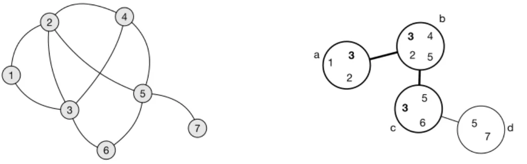
Figure 1 Example undirected, unlabeled, graph (left) and decomposition of width 3 (right).
3. ∀v ∈ V , {i ∈ I | v ∈ B(i)} induces a subtree of T .
Intuitively, a tree decomposition groups the vertices of a graph into bags so that they form a tree-like structure, where a link between bags is established when there exists common vertices in both bags.
IExample 2. Figure 1 illustrates such a decomposition. The resulting decomposition is
formed of 4 bags, each containing a subset of the nodes in the graph. The bags containing node 3 (in bold) form a connected subtree of the tree decomposition.
Based on the number of vertices in a bag, we can define the concept of treewidth:
IDefinition 3 ((Treewidth)). Given a graph G = (V, E) the width of a tree decomposition
(T, B) is equal to maxi∈I(|B(i)| − 1). The treewidth of G, w(G), is equal to the minimal
width of all tree decompositions of G.
It is easy to see that an isolated point has treewidth 0, a tree treewidth 1, a cycle treewidth 2, and a (k + 1)-clique (a complete graph of k nodes) treewidth k.
IExample 4. The width of the decomposition in Figure 1 is 3. This tells us the graph
has a treewidth of at most 3. The treewidth of this graph is actually exactly 3: indeed, the 4-clique, which has treewidth 3, is a minor of the graph in Figure 1 (it is obtained by removing nodes 1 and 7, and by contracting the edges between 3 and 6 and 5 and 6), and treewidth never increases when taking a minor (see, for instance, [38]).
As previously mentioned, the treewidth of an arbitrary relational instance is defined as that of its Gaifman graph, the graph whose vertices are constants of the instances and where there is an edge between two vertices if they co-occur in the same fact. We will therefore implicitly represent relational database instances by their Gaifman graphs in what follows.
We are now ready to present algorithms for lower and upper bounds on treewidth.
3
Treewidth Estimation
The objective of our experimental evaluation is to obtain reasonable estimations of treewidth, using algorithms with reasonable execution time on real-world graphs.
Once we know we do not have the luxury of an exact computation of the treewidth, we are left with estimations of the range of possible treewidths, between a lower bound and an upper bound. For the purposes of this experimental survey, we restrict ourselves to the most efficient estimation algorithms from the literature. We refer the reader to [19] and [20], respectively, for a more complete survey of treewidth upper and lower bound estimation algorithms on synthetic data.
1 4 6 5 3 2 7 7 1 6 3 5 2 4
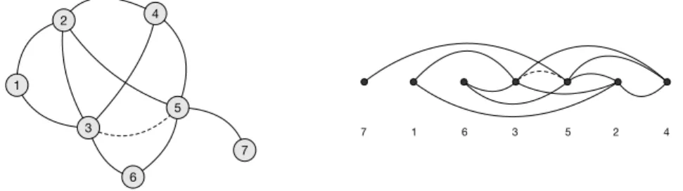
Figure 2 Graph triangulation for the graph of Figure 1 (left) and its elimination ordering (right).
Treewidth Upper Bounds. As we have defined, the treewidth is the smallest width among
all possible tree decompositions. In other words, the width of any decomposition of a graph is an upper bound of the actual treewidth of that graph. A treewidth upper bound estimation algorithm can thus be seen as an algorithm to find a decomposition whose width is as close as possible to the treewidth of the graph. To understand how one can do that, we need to introduce the classical concept of elimination ordering and to explain its connection to treewidth.
We start by introducing triangulations of graphs, which transform a graph G into a graph G∆that is chordal:
IDefinition 5. A chordal graph is a graph G such that every cycle in G of at least four
vertices has a chord – an edge between two non-successive vertices in the cycle.
A triangulation (or chordal completion) of a graph G is a minimal chordal supergraph
G∆ of G: a graph obtained from G by adding a minimal set of edges to obtain a chordal
graph.
IExample 6. The graph in Figure 1 is not chordal, since, for example, the cycle 3–4–5–6–3
does not have a chord. If one adds an edge between 3 and 5, as in Figure 2 (left), one can verify that the resulting graph is chordal, and thus a triangulation of the graph of Figure 1. One way to obtain triangulations of graphs is elimination orderings. An elimination ordering ω of a graph G = (V, E) of n nodes is an ordering of the vertices of G, i.e., it can be seen as a bijection from V onto {1, . . . , n}. From this ordering, one obtains a triangulation by applying sequentially the following elimination procedure for each vertex v: first, edges are added between remaining neighbors of v as needed so that they form a clique, then v is
eliminated (removed) from the graph. For every elimination ordering ω, G along with all
edges added to G in the elimination procedure forms a graph, denoted G∆
ω. This graph is
chordal (indeed, we know that the two neighbors of the first node of any cycle we encounter in the elimination ordering have been connected by a chord by the elimination procedure). It is also a supergraph of G, and it can be shown it is a minimal chordal supergraph, i.e., a triangulation of G.
IExample 7. Figure 2 (right) shows a possible elimination ordering (7, 1, 6, 3, 5, 2, 4) of the
graph of Figure 1. The elimination procedure adds a single edge, when processing node 6, between nodes 3 and 5. The resulting triangulation is the graph on the left of Figure 2.
ITheorem 8. [19] Let G = (V, E) a graph, and k 6 n. The following are equivalent:
1. G has treewidth k.
2. G has a triangulation G∆, such that the maximum clique in G∆ has size k + 1.
3. There exists an elimination ordering ω such that the maximum clique size in G∆
ω is k + 1.
Obtaining the treewidth of the graph is thus equivalent to finding an optimal elimination ordering. Moreover, constructing a tree decomposition from an elimination ordering is a natural process: each time a vertex is processed, a new bag is created containing the vertex and its neighbors. Note that, in practice, we do not need to compute the full elimination ordering: we can simply stop when we know that the number of remaining vertices is lower that the largest clique found thus far.
I Example 9. In the triangulation of Figure 2 (left), corresponding to the elimination
ordering on the right, the maximum clique has size 4: it is induced by the vertices 2, 3, 4, 5. This proves the existence of a tree decomposition of width 3. Indeed, it is exactly the tree decomposition in Figure 1 (right): bag d is constructed when 7 is eliminated, bag a when 1 is eliminated, bag c when 6 is eliminated, and finally bag b when 3 is eliminated.
Finding a “good” upper bound on the treewidth can thus be done by finding a “good” elimination ordering. This is still an intractable problem, of course, but there are various heuristics for generating elimination orderings leading to good treewidth upper bounds. One important class of such elimination ordering heuristics are the greedy heuristics. Intuitively, the elimination ordering is generated in an incremental manner: each time a new node has to be chosen in the elimination procedure, it is chosen using a criterion based on its neighborhood. In our study, we have implemented the following greedy criteria (with ties broken arbitrarily):
Degree. The node with the minimum degree is chosen. [49, 16]
FillIn. The node with the minimum needed “fill-in” (i.e., the minimum number of missing edges for its neighbors to form a clique) is chosen. [19]
Degree+FillIn. The node with the minimum sum of degree and fill-in is chosen.
IExample 10. The elimination ordering of Figure 2 (right) is an example of the use of
Degree+FillIn. Indeed, 7 is first chosen, with value 1, then 1 with value 2, then 6 with value 2 + 1 = 3. After that, the order is arbitrary since 2, 3, 4, and 5 form a clique (and thus have initial value 3).
Previous studies [59, 42, 19] have found these greedy criteria give the closest estimations of the real treewidth. An alternative way of generating an elimination ordering is based on maximum cardinality search [42, 19]; however, it is both less precise than the greedy algorithms – due to its reliance on how the first node in the ordering is chosen – and slower to run.
Treewidth Lower Bounds. In contrast to upper bounds, obtaining treewidth lower bounds
is not constructive. In other words, lower bounds do not generate decompositions; instead, the estimation of a lower bound is made by computing other measures on a graph, that are a proxy for treewidth. In this study, we implement algorithms using three approaches: subgraph-based bounds, minor-based bounds, and bounds obtained by constructing improved graphs.
Given a graph G = (V, E), let δ(G) be its lowest degree, and δ2(G)> δ(G) its second
lowest degree (i.e., the degree of the second vertex when ordered by degree). It is known that δ2(G) is itself a lower bound on the treewidth [43]. This, however, is too coarse an
estimation, and we need better bounds. We shall use two degeneracy measures of the graphs. The first, the degeneracy of G, δD(G), is the maximum value of δ(H) over all subgraphs H of G. Similarly, the δ2-degeneracy, δ2D(G), of a graph is the maximum value of δ2(H) over
all subgraphs H.
We have the following lemma:
ILemma 11. [20] Let G = (V, E) be a graph, and W ⊆ V be a set of vertices. The treewidth
of the subgraph of G induced by W is at most the treewidth of G.
A corollary of the above lemma is that the values δD(G) and δ2D(G) are themselves
lower bounds of treewidth:
ICorollary 12. [20] For every graph G, the treewidth of G is at least δ2D(G) > δD(G).
To compute δD(G) and δ2D(G) exactly, the following natural algorithms can be used
[43, 20]: repeatedly remove a vertex of smallest degree – or smallest except for some fixed node v, respectively – from the graph, and keep the maximum value thus encountered. As in [20], we refer to these algorithms as Mmd (Maximum Minimum Degree) and Delta2D, respectively. Ties are broken arbitrarily.
I Example 13. Let us apply the Mmd algorithm to the graph of Figure 1 (left). The
algorithm may remove, in order, 7 (degree 1), 1 (degree 2), 6 (degree 2), 3 (degree 2), 5 (degree 2), 4 (degree 1), 2 (degree 0). This gives a lower bound of 2 on the treewidth, which
is not tight as we saw.
An equivalent of Lemma 11 on treewidth also holds for minors of a graph G: if H is a minor of G, then the treewidth of H is at most the treewidth of G [38]. A minor H of a graph G is a graph obtained by allowing, in addition to edge and node deletion as when taking subgraphs, edge contractions. Then the concepts of contraction degeneracy, δC(G), and δ2-contraction degeneracy, δ2C(G), are defined analogously to δD(G) and δ2D(G) by
considering all minors instead of all subgraphs:
ILemma 14. [20] For every graph G, the treewidth of G is at least δ2C(G) > δC(G).
Unfortunately, computing δC(G) or δ2C(G) is NP-hard [21]; hence, only heuristics can
be used. One such heuristic for δC(G) is a simple change to the Mmd algorithm, called Mmd+ [21, 36]: at each step, instead of removing a vertex, a neighbor is chosen and the corresponding edge is contracted. Choosing a neighbor node to contract requires some heuristic also; in line with previous studies, in this study we choose the neighbor node that has the least overlap in neighbors – this is called the least-c heuristic [63].
Finally, another approach to treewidth lower bounds that we consider are improved
graphs, an approach that can be used in combination with any of the lower bound estimation
algorithms presented so far. Consider a graph G and an integer k and the following operation: while there are non-adjacent vertices v and w that have at least k + 1 common neighbors, add the edge (v, w) to the improved graph G0. The resulting graph G0is the (k + 1)-neighbor improved graph of G. Using these improved graphs can lead to a lower bound on treewidth: the (k + 1)-neighbor improved graph G0 of a graph G having at most treewidth k also has
treewidth at most k.
To use this property, one can start from an already computed estimation k of a lower bound (by using Mmd, Mmd+, or Delta2D for example) and then repeatedly generate a (k + 1)-neighbor improved graph, estimate a new lower bound on treewidth, and repeat the process until the graph cannot be improved. This algorithm is known as Lbn in the
literature [23], and can be combined with any other lower bound estimation algorithm. A refinement of Lbn, that alternates improvement and contraction steps, Lbn+, has also been proposed [21].
IExample 15. Let us illustrate the use of Lbn together with Mmd on the graph of Figure 1
(left). As shown in Example 13, a first run of Mmd yields k = 2. We compute a 3-neighbor improved graph for G by adding an edge between nodes 3 and 5 (that share neighbors 2, 4, 6). Now, running Mmd one more time yields the possible sequence 7 (degree 1), 1 (degree 2), 6 (degree 2), 3 (degree 3), 5 (degree 2), 4 (degree 1), 2 (degree 0). We thus obtain a lower bound of 3 on the treewidth, which is this time tight.
4
Estimation Results
We now present our main experimental study, first introducing the 25 datasets we are considering, then upper and lower bound results, running time and estimators, and an aside discussion of the treewidth of synthetic networks. All experiments were made on a server using an 8-core Intel Xeon 1.70GHz CPU, having 32GB of RAM, and using 64bit Debian Linux. All datasets were given at least two weeks to finish, after which the algorithms were stopped and the best lower and upper bounds were recorded.
Datasets. For our study, we have evaluated the treewidth estimation algorithms on 25
datasets from 8 different domains (see Appendix A of [48] for descriptions of how they were obtained): infrastructure networks (road networks, public transportation, power grid), social networks (explicit as in social networking sites, or derived from interaction patterns), web-like networks, a communication network, data with a hierarchical structure (genealogy trees), knowledge bases, traditional OLTP data, as well as a biological interaction network.
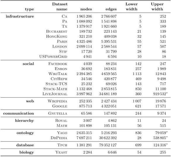
Table 1 summarizes the datasets, their size, and the best treewidth estimations we have been able to compute. For reproducibility purposes, all datasets, along with the code that has been used to compute the treewidth estimations, can be freely downloaded from https://github.com/smaniu/treewidth/.
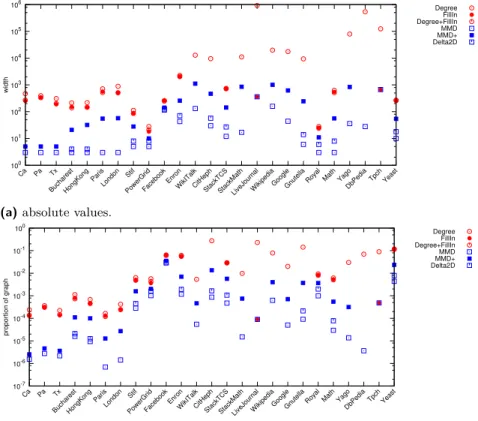
Upper Bounds. We show in Figure 3 the results of our estimation algorithms. Lower values
mean better treewidth estimations. Focusing on the upper bounds only (red circular points), we notice that, in general, FillIn does give the smallest upper bound of treewidth, in line with previous findings [20]. Interestingly, the Degree heuristic is quite competitive with the other heuristics. This fact, coupled with its lower running time, means that it can be used more reliably in large graphs. Indeed, as can be seen in the figure, on some large graphs only the Degree heuristic actually finished at all; this means that, as a general rule, Degree seems the best fit for a quick and relatively reliable estimation of treewidth.
We plot both the absolute values of the estimations in Figure 3a, but also their relative values (in Figure 3b, representing the ratio of the estimation over the number of nodes in the graph), to allow for an easier comparison between networks. The absolute value, while interesting, does not yield an intuition on how the bounds can differ between network types. If we look at the relative values of treewidth, it becomes clear that infrastructure networks have a treewidth that is much lower than other networks; in general they seem to be consistently under one thousandth of the original size of the graph. This suggests that, indeed, this type of network may have properties that make them have a lower treewidth. For the other types of networks, the estimations can vary considerably: they can go from one hundredth (e.g., Math) to one tenth (e.g., WikiTalk) of the size of the graph.
Table 1 Datasets and summary of lower and upper bounds. Bounds with a∗are partial (the decomposition process was interrupted before it finished).
Dataset Lower Upper
type name nodes edges width width
infrastructure Ca 1 965 206 2 766 607 5 252 Pa 1 088 092 1 541 898 5 333 Tx 1 379 917 1 921 660 5 189 Bucharest 189 732 223 143 21 139 HongKong 321 210 409 038 32 145 Paris 4 325 486 5 395 531 55 521 London 2 099 114 2 588 544 57 507 Stif 17 720 31 799 28 86 USPowerGrid 4 941 6 594 10 18 social Facebook 4 039 88 234 142 247 Enron 36 692 183 831 257 1 989 WikiTalk 2 394 385 4 659 565 1 113 12 843 CitHeph 34 546 420 877 469 9 498 Stack-TCS 25 232 69 026 143 717 Stack-Math 1 132 468 2 853 815 850 11 100 LiveJournal 3 997 962 34 681 189 360 919 532∗ web Wikipedia 252 335 2 427 434 1 007 19 876 Google 875 713 4 322 051 621 17 571 communication Gnutella 65 586 147 892 244 9 374 hierarchy Royal 3 007 4 862 11 24 Math 101 898 105 131 56 515 ontology Yago 2 635 315 5 216 293 836 79 059∗ DbPedia 7 697 211 30 622 392 28 538 805∗ database Tpch 1 381 291 79 352 127 699 124 316∗ biology Yeast 2 284 6 646 54 255
As further explained in Appendix B of [48], the bounds obtained here on infrastruc-ture networks are consistent with a conjecinfrastruc-tured O(√3n) bound on the treewidth of road
networks [27]. One relevant property is their low highway dimension [2], which helps with routing queries and decomposition into contraction hierarchies. Even more relevant to our results is the fact that they tend to be “almost planar”. More specifically, they are k-planar: each edge can allow up to k crossing in their plane embedding. It has been shown in [28] that
k-planar graphs have treewidth O(p(k + 1)n), a relatively low treewidth that is consistent
with our results.
The treewidth of hierarchical networks is surprisingly high, but not for trivial reasons: in both Royal and Math, largest cliques have size 3. More complex structures (cousin marriages, scientific communities) impact the treewidth, along with the fact that treewidth cannot exploit the property that both networks are actually DAGs.
In upper bound algorithms, ties are broken arbitrarily which causes a non-deterministic behavior. We show in Appendix C of [48] that variations due to this non-determinism is of little significance.
100 101 102 103 104 105 106 Ca Pa Tx BucharestHongKong Paris London Stif PowerGridFacebook Enron
WikITalkCitHephStackTCSStackMath
LiveJournalWikipediaGoogleGnutella Royal Math Yago
DbPediaTpch Yeast width Degree FillIn Degree+FillIn MMD MMD+ Delta2D
(a) absolute values.
10-7 10-6 10-5 10-4 10-3 10-2 10-1 100 Ca Pa Tx BucharestHongKong Paris London Stif PowerGridFacebook Enron WikITalkCitHephStackTCS
StackMathLiveJournalWikipediaGoogleGnutella Royal Math Yago
DbPediaTpch Yeast proportion of graph Degree FillIn Degree+FillIn MMD MMD+ Delta2D (b) relative values.
Figure 3 Treewidth estimation of different algorithms (logarithmic scale).
Lower Bounds. Figure 3 also reports on the lower bound estimations (blue rectangular
points). Now, higher values represent a better estimation. The same differentiation between infrastructure networks and the other networks holds in the case of lower bounds – treewidth lower bounds are much lower in comparison with other networks. We observe that the variation between upper and lower bound estimations can be quite large. Generally, we find that degree-based estimators, Mmd and Delta2D, give bounds that are very weak. The contraction-based estimator, Mmd+, however, consistently seems to give the best bounds of treewidth, and returns lower bounds that are much larger than the degree-based estimations.
Interestingly, in the case of the networks Ca, Pa, and Tx, the values returned for Mmd+ and Mmd are always 5 and 3, respectively. This has been remarked on in [21] – there exist instances where heuristics of lower bounds perform poorly, giving very low lower bounds. In our case, this only occurs for some road networks, all coming from the same data source, i.e., the DIMACS challenge on shortest paths.
In Figure 3, we have not plotted the estimations resulting from Lbn and Lbn+. The reason is that we have found that these algorithms do not generally give any improvement in the estimation of the lower bounds. Specifically, we have found an improvement only in two datasets for the Delta2D heuristic: for Facebook from 126 originally to 157 for Lbn(Delta2D) and 159 for Lbn+(Delta2D); and for Stack-TCS from 27 originally to 30 for Lbn+(Delta2D). In all cases, however, Mmd+ is always competitive by itself.
Running Time. The complexity of different estimation algorithms (see Appendix D of [48]),
varies a lot, ranging from quasi-linear for low-treewidth to cubic time. Even if all of the algorithms exhibit polynomial complexity, the cost can become quickly prohibitive, even for
graphs of relatively small sizes; indeed, not all algorithms finished on all datasets within the time bound of two weeks of computation time: indeed, only the fastest algorithms for each bound – Degree and Mmd respectively – finish processing all datasets. In some cases, for upper bounds, even Degree timed out – in this case, we took the value found at the moment of the time-out; this still represents an upper bound. The datasets for which this occurred are LiveJournal, Yago, DbPedia, and Tpch.1
Phase Transitions in Synthetic Networks. We have seen that graphs other than the
infrastructure networks have treewidth values that are relatively high. An interesting question that these results lead to is: is it the case for all relatively complex networks, or is
it a particularity of the chosen datasets?
To give a possible answer to this, we have evaluated the treewidth of a range of synthetic graph models and their parameters:
Random. This synthetic network model due to Erdős and Rényi [30] is an entirely random one: given n nodes and a parameter p ∈ (0, 1], each possible edge between the n nodes is added with probability p. We have generated several network of n = 10 000 nodes, and with values of p ranging from 10−5 to 10−3.
Preferential Attachment. This network model [6] is a generative model, and aims to simulate link formation in social networks: each time a new node is added to the network, it attaches itself to m other nodes, each link being formed with a probability proportional to the number of neighbors the existing node already has. We have generated graphs of
n = 10 000 nodes, with the parameter m varying between 1 and 20.
Small-World. The model [61] generates a small-world graph by the following process: first, the n nodes are organized in a ring graph where each node is connected with m other nodes on each side; finally, each edge is rewired (its endpoints are changed) with probability p. In the experiments, we have generated graphs of n = 10 000, with p = {0.1, 0.2, 0.5} and
m ranging between 1 and 20.
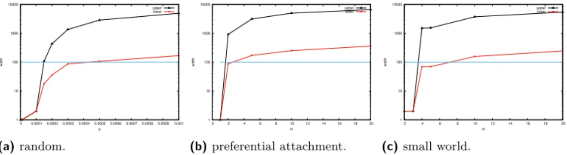
Our objective with evaluating treewidth on these synthetic instances is to evaluate whether some parameters of these models lead to lower treewidth values, and if so, in which model the “phase transition” occurs, i.e., when a low-treewidth regime gives way to a high-treewidth one. For our purpose, and for reasons we explain in Section 5, we consider a treewidth under √
n to be low.
Our first finding – see Figure 4 – is that the high-treewidth regime arrives very early, relative to the parameter values. For random graphs, only relatively small value of p allow for a low treewidth; for small-world and preferential attachment only trivial values of m allow low-treewidth – and, even so, it is usually 1 or 2, possibly due to the fact that the graph, in those cases, is composed of several small connected components, i.e., the well-known subcritical regime of random graphs [15]. The low-treewidth regime for random networks seems to be limited to values immediately after p =n1; after this point, the treewidth is high, in line with findings of a linear dependency between graph size and treewidth in random graphs [35]. Moreover, we notice that there is no smooth transition for preferential attachment and small world networks; the treewidth jumps from very low values to high treewidth values. This is understandable in scale-free networks – resulting from the preferential attachment
1 We show in Figure 9 of Appendix D of [48] the full running time results for the upper and lower bound
1 10 100 1000 10000 0 0.0001 0.0002 0.0003 0.0004 0.0005 0.0006 0.0007 0.0008 0.0009 0.001 width p upper lower (a) random. 1 10 100 1000 10000 0 2 4 6 8 10 12 14 16 18 20 width m upper lower (b) preferential attachment. 1 10 100 1000 10000 2 4 6 8 10 12 14 16 18 20 width m upper lower (c) small world.
Figure 4 Lower and upper bounds of treewidth in synthetic networks, as a function of generator
parameters. The blue line represent the low width regime, where treewidth is less than 100.
model – where a few hubs may exist with degrees that are comparable to the number of nodes in the graph. Comparatively, random networks exhibit a smoother progression – one can clearly see the shift from trivial values of treewidth, to relatively low values, and to high treewidth values. Finally, the gap between lower bound and upper bound tends to increase with the parameter; that is, however, not surprising since all three model graphs tend to have more edges with larger parameter values.
5
Partial Decompositions
Our results show that, in practice, the treewidths of real networks are quite high. Even in the case of road networks, having relatively low treewidths, their value can go in the hundreds, rendering most algorithms whose time is exponential time in the treewidth (or worse) unusable. In practical applications, however, we can still adapt treewidth-based approaches for obtaining data structures – not unlike indexes – which can help with some important graph queries like shortest distances and paths [62, 5] or probability estimations [47, 10].
The manner in which treewidth decomposition can be used starts from a simple observation made in studies on complex graphs, that is, that they tend to exhibit a tree-like fringe and a densely connected core [52, 51]. The tree-like fringe precisely corresponds to bounded-treewidth parts of the network. This yields an easy adaptation of the upper bound algorithms based on node ordering: given a parameter w representing the highest treewidth the fringe can be, we can run any greedy decomposition algorithm (Degree, FillIn, DegreeFillIn) until we only find nodes of degree w + 1, at which point the algorithm stops. At termination, we obtain a data structure formed of a set of treewidth w elements (w-trees) interfacing through cliques that have size at most w + 1 with a core graph. The core graph contains all the nodes not removed in the bag creation process, and has unbounded treewidth. Figure 5 illustrates the notion of partial decompositions.
The resulting structure can be thought of as a partial decomposition (or relaxed
decom-position), a concept introduced in [62, 5] in the context of answering shortest path queries,
and used in [47] for probabilistic distance queries. A partial decomposition can be extremely useful. The tree-like fringe can be used to quickly precompute answers to partial queries (e.g., precompute distances in the graph). Once the precomputation is done, these (partial) answers are added to the core graph, where queries can be answered directly. If the resulting core graph is much smaller than the original graph, the gains in running time can be considerable, as shown in [62, 5, 47]. Hence, the objective of our experiments in this section is to check how feasible partial decompositions are.
core w-tre e (w=3) w-tree (w =4) w-t ree ( w=1) fringe
Figure 5 An abstract view of partial decompositions. Partial decompositions are formed of a
core graph, which interfaces with w-trees through w-cliques (the fringe).
An interesting aspect of greedy upper bound algorithms is that they generate at any point a partial decomposition, with width equal to the highest degree encountered in the greedy ordering so far. The algorithm can then be stopped at any width, and the size of the resulting partial decomposition can be measured.
To evaluate this, we track here the size of the core graph, in terms of edges. We do this because most algorithms on graphs have a complexity that is directly related to the number of edges in the graph. As we discussed in the previous section, we aim that the size of the core graph to be as small as possible. Another aspect to keep in mind is the number of edges that are added by the fill-in process during the decomposition: each time a node of degree w is removed, at most w(w−1)2 edges are added to the graph. Finally, for a graph of treewidth k, the decomposition contains a root of size at most k2edges. Hence, to ensure that the core
graph is smaller than the original graph we aim for the treewidth to be√n. As we saw in
Section 4, this is only rarely the case, and it is more likely to occur in infrastructure networks.
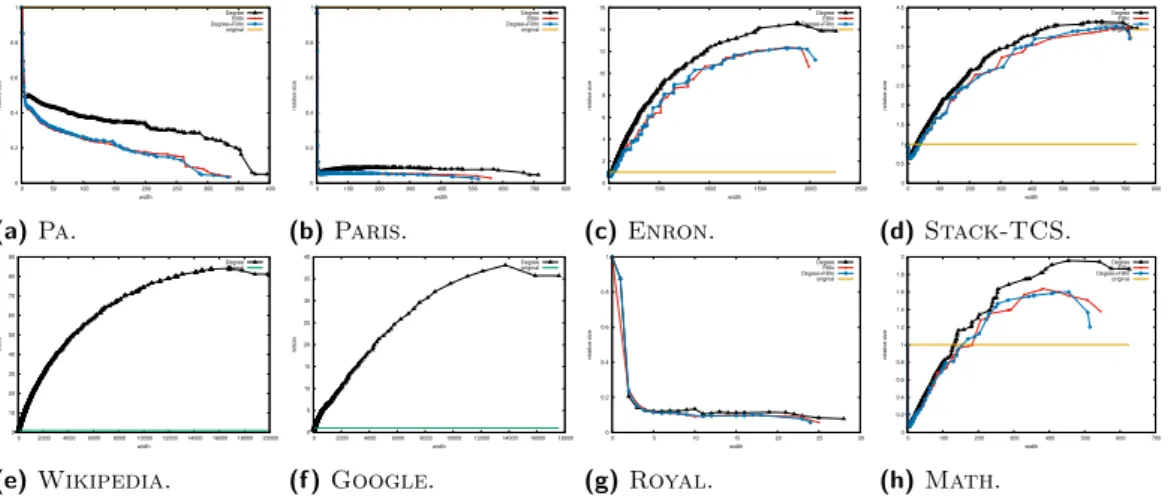
0 0.2 0.4 0.6 0.8 1 0 50 100 150 200 250 300 350 400 relative size width Degree FillIn Degree+FillIn original (a) Pa. 0 0.2 0.4 0.6 0.8 1 0 100 200 300 400 500 600 700 800 relative size width Degree FillIn Degree+FillIn original (b) Paris. 0 2 4 6 8 10 12 14 16 0 500 1000 1500 2000 2500 relative size width Degree FillIn Degree+FillIn original (c) Enron. 0 0.5 1 1.5 2 2.5 3 3.5 4 4.5 0 100 200 300 400 500 600 700 800 relative size width Degree FillIn Degree+FillIn original (d) Stack-TCS. 0 10 20 30 40 50 60 70 80 90 0 2000 4000 6000 8000 10000 12000 14000 16000 18000 20000 relsize width Degree original (e) Wikipedia. 0 5 10 15 20 25 30 35 40 0 2000 4000 6000 8000 10000 12000 14000 16000 18000 relsize width Degree original (f ) Google. 0 0.2 0.4 0.6 0.8 1 0 5 10 15 20 25 30 relative size width Degree FillIn Degree+FillIn original (g) Royal. 0 0.2 0.4 0.6 0.8 1 1.2 1.4 1.6 1.8 2 0 100 200 300 400 500 600 700 relative size width Degree FillIn Degree+FillIn original (h) Math.
Figure 6 Relative sizes of core graphs in partial decompositions, after all bags of a given size
Indeed, if we plot the core graph size in the partial decompositions of infrastructure networks (Figures 6a, 6b), we see that their size is only a fraction of the original size. We see a large drop in the size for low widths; this is logical, since the fill-in process does not add edges for w = 1 and w = 2. After this point, the size is relatively stable, and can go as low as 10% of the original size. In this sense, infrastructure networks seem the best fit for indexes based on decompositions, and represents further confirmation of the good behavior of these networks for hierarchical decompositions.
This desired decomposition behavior no longer occurs for social networks (Figures 6c, 6d) and the other networks in our dataset (Figures 6e, 6f). In this case, the decomposition becomes too large and even unwieldy – for some networks, the decomposition started filling the main memory of our computers (32 GB of RAM); for other networks, they did not finish in reasonable time (i.e., a few days of computation). For most of these networks, the resulting treewidth is much larger than our desired bound of at most√n); this results in core graph
sizes that can be hundreds of times larger than the original size. The only exceptions are hierarchical networks, Royal and Math (Figures 6g, 6h), which are after all supposed to be close to a tree – despite having a relatively high treewidth (remember Figure 3b), partial decompositions work well on them. See Appendix E of [48] for full results.
In practice, however, we do not need to compute full decompositions. For usable indexes, we may want to stop at low treewidths, which allow exact computing. This may be useful for graphs whose decompositions have large core graphs. Indeed (see Appendix G of [48] for details), by stopping at width between 5 and 10, it is often possible to significantly reduce the original size of the graph, even in cases where core graphs are large, such as the Google graph.
Such partial decompositions are an extremely promising tool: on databases where partial decomposition result in a core graph of reduced size, efficient algorithms can be run on the fringe, exploiting its low treewidth, while more costly algorithms are used on the core, which has reduced size. Combining results from the fringe and the core graph can be a challenging process, however, which is worth investigating for separate problems. As a start, we have shown in [47] how to exploit partial decompositions to significantly improve the running time of source-to-target queries in probabilistic graphs.
6
Discussion
In this article, we have estimated the treewidth of a variety of graph datasets from different domains, and we have studied the running time and effectiveness of estimation algorithms. This study was motivated by the central role treewidth plays in many theoretical work attacking query evaluation tasks that are otherwise intractable, where low treewidths are an indicator for low complexity.
Our study on the algorithms for estimation leads to results that may seem surprising. For upper bounds, we discovered that greedy treewidth estimators, based on elimination orderings, provide the best cost–estimation trade-off; they also have the advantage of outputting readily-usable tree decompositions. In the case of lower bounds, we discovered that degeneracy-based bounds display the best behavior; moreover, the algorithms which aim to improve the bounds (LBN and LBN+) only very rarely do so.
In terms of treewidth estimations, we have discovered that, generally, the treewidth of real-world graphs is quite large. With few exceptions, most of the graphs we have tested in this study are scale-free. This may partly explain our findings – scale-free networks exhibit a number of high-degree, or hub, nodes that force high values for the treewidth. The few
exceptions to this rule are infrastructure networks, where treewidths are comparatively lower. Indeed, we were able to reproduce a O(√3n) bound on the treewidth of road networks. We
conjecture these relatively low bounds are explained by characteristics of infrastructure networks: specifically, they are similar to very sparse random networks.
Even in the case of infrastructure networks, the absolute value of treewidth still renders algorithms that are exponential in the treewidth impractical. However, one of the main lesson of this work is that it is still possible to exploit the structure of such datasets, by computing partial tree decompositions: following the approach of Section 5, it is often possible to decompose a dataset into a fringe of low treewidth and a smaller core of high treewidth. This has been used in [47], but for a very specific (and limited) application: connectivity queries in probabilistic graphs.
In brief, though low-treewidth data guarantees a wealth of theoretical results on the tractability of various data management tasks, this is unexploitable in most real-world datasets, which do not have low enough treewidth. One direction is of course to find relaxations of the treewidth notion, such as in [33, 41]. But since low treewidth is sometimes the only notion that ensures tractability [45, 34, 9], other approaches are needed; a promising one lies in the notion of partial tree decompositions. We believe future work in database theory should study in more detail the nature of partial tree decompositions, how to obtain optimal or near-optimal partial decompositions, and how to exploit them for improving the efficiency of a wide range of data management problems, from query evaluation, to enumeration, probability estimation, or knowledge compilation.
References
1 Serge Abiteboul, Richard Hull, and Victor Vianu. Foundations of databases. Addison-Wesley,
1995.
2 Ittai Abraham, Amos Fiat, Andrew V Goldberg, and Renato F Werneck. Highway dimension,
shortest paths, and provably efficient algorithms. In SODA, 2010.
3 Aaron B. Adcock, Blair D. Sullivan, and Michael W. Mahoney. Tree decompositions and social
graphs. Internet Mathematics, 12(5), 2016.
4 M. Ajtai, R. Fagin, and L. J. Stockmeyer. The Closure of Monadic NP. JCSS, 60(3), 2000.
5 Takuya Akiba, Christian Sommer, and Ken-ichi Kawarabayashi. Shortest-Path Queries for
Complex Networks: Exploiting Low Tree-width Outside the Core. In EDBT, 2012.
6 Réka Albert and Albert-László Barabási. Statistical mechanics of complex networks. Rev.
Mod. Phys., 74, 2002.
7 Antoine Amarilli, Pierre Bourhis, Louis Jachiet, and Stefan Mengel. A Circuit-Based Approach
to Efficient Enumeration. In ICALP, 2017.
8 Antoine Amarilli, Pierre Bourhis, and Pierre Senellart. Provenance Circuits for Trees and
Treelike Instances. In ICALP, 2015.
9 Antoine Amarilli, Pierre Bourhis, and Pierre Senellart. Tractable Lineages on Treelike Instances:
Limits and Extensions. In PODS, 2016.
10 Antoine Amarilli, Silviu Maniu, and Mikaël Monet. Challenges for Efficient Query Evaluation
on Structured Probabilistic Data. In SUM, 2016.
11 Antoine Amarilli, Mikaël Monet, and Pierre Senellart. Connecting Width and Structure in
Knowledge Compilation. In ICDT, pages 6:1–6:17, 2018. doi:10.4230/LIPIcs.ICDT.2018.6.
12 Eyal Amir. Approximation Algorithms for Treewidth. Algorithmica, 56(4):448–479, 2010.
13 Stefan Arnborg, Derek G. Corneil, and Andrzej Proskuworski. Complexity of finding
embed-dings in a k-tree. SIAM Journal on Algebraic and Discrete Methods, 8(2), 1987.
14 Guillaume Bagan. MSO queries on tree decomposable structures are computable with linear
15 Albert-László Barabási and Márton Pósfai. Network science. Cambridge University Press, 2016.
16 Anne Berry, Pinar Heggernes, and Geneviève Simonet. The Minimum Degree Heuristic and the
Minimal Triangulation Process. Graph-Theoretic Concepts in Computer Science, 2880(Chapter 6), 2003.
17 Hans L. Bodlaender. A Linear-Time Algorithm for Finding Tree-Decompositions of Small
Treewidth. SIAM J. Comput., 25(6), 1996.
18 Hans L. Bodlaender, Fedor V Fomin, Arie M C A Koster, Dieter Kratsch, and Dimitrios M
Thilikos. On exact algorithms for treewidth. ACM TALG, 9(1), 2012.
19 Hans L. Bodlaender and Arie M C A Koster. Treewidth Computations I. Upper Bounds.
Information and Computation, 208(3), 2010.
20 Hans L. Bodlaender and Arie M C A Koster. Treewidth Computations II. Lower Bounds.
Information and Computation, 209(7), 2011.
21 Hans L. Bodlaender, Arie M. C. A. Koster, and Thomas Wolle. Contraction and Treewidth
Lower Bounds. In ESA, 2004.
22 Angela Bonifati, Wim Martens, and Thomas Timm. An Analytical Study of Large SPARQL
Query Logs. PVLDB, 11(2), 2017.
23 François Clautiaux, Jacques Carlier, Aziz Moukrim, and Stéphane Nègre. New Lower and
Upper Bounds for Graph Treewidth. In WEA, 2003.
24 Bruno Courcelle. The Monadic Second-Order Logic of Graphs. I. Recognizable Sets of Finite
Graphs. Inf. Comput., 85(1), 1990.
25 Nilesh N. Dalvi and Dan Suciu. The dichotomy of conjunctive queries on probabilistic
structures. In PODS, 2007.
26 Holger Dell, Christian Komusiewicz, Nimrod Talmon, and Mathias Weller. The PACE 2017
Parametrized Algorithms and Computation Experiments Challenge: The Second Iteration. In
IPEC, 2017.
27 Julian Dibbelt, Ben Strasser, and Dorothea Wagner. Customizable Contraction Hierarchies.
Journal of Experimental Algorithmics, 21(1), 2016.
28 Vida Dujmović, David Eppstein, and David R Wood. Structure of Graphs with Locally
Restricted Crossings. SIAM J. Discrete Maths, 31(2), 2017.
29 Arnaud Durand and Yann Strozecki. Enumeration Complexity of Logical Query Problems
with Second-order Variables. In CSL, 2011.
30 Paul Erdős and Alfréd Rényi. On Random Graphs I. Publicationes Mathematicae (Debrecen),
6, 1959.
31 Johannes K. Fichte, Neha Lodha, and Stefan Szeider. SAT-Based Local Improvement for
Finding Tree Decompositions of Small Width. In Serge Gaspers and Toby Walsh, editors,
Theory and Applications of Satisfiability Testing – SAT 2017, 2017.
32 Jörg Flum, Markus Frick, and Martin Grohe. Query evaluation via tree-decompositions. J.
ACM, 49(6), 2002.
33 Markus Frick and Martin Grohe. Deciding first-order properties of locally tree-decomposable
structures. J. ACM, 48(6), 2001.
34 Robert Ganian, Petr Hliněn`y, Alexander Langer, Jan Obdržálek, Peter Rossmanith, and
Somnath Sikdar. Lower bounds on the complexity of MSO1 model-checking. JCSS, 1(80), 2014.
35 Yong Gao. Treewidth of Erdős–Rényi random graphs, random intersection graphs, and
scale-free random graphs. Discrete Applied Mathematics, 160(4–5), 2012.
36 Vibhav Gogate and Rina Dechter. A Complete Anytime Algorithm for Treewidth. In UAI,
2004.
37 Martin Grohe, Thomas Schwentick, and Luc Segoufin. When is the Evaluation of Conjunctive
Queries Tractable? In STOC, 2001.
38 Daniel John Harvey. On Treewidth and Graph Minors. PhD thesis, The University of
39 Abhay Jha and Dan Suciu. On the Tractability of Query Compilation and Bounded Treewidth. In ICDT, 2012.
40 Abhay Kumar Jha and Dan Suciu. Knowledge Compilation Meets Database Theory: Compiling
Queries to Decision Diagrams. Theory Comput. Syst., 52(3), 2013.
41 Wojciech Kazana and Luc Segoufin. Enumeration of first-order queries on classes of structures
with bounded expansion. In PODS, 2013.
42 Daphne Koller and Nir Friedman. Probabilistic Graphical Models: Principles and Techniques.
The MIT Press, 2009.
43 Arie M. C. A. Koster, Thomas Wolle, and Hans L. Bodlaender. Degree-Based Treewidth
Lower Bounds. In WEA, 2005.
44 Stephan Kreutzer. Algorithmic Meta-Theorems. CoRR, abs/0902.3616, 2009.
45 Stephan Kreutzer and Siamak Tazari. Lower bounds for the complexity of monadic second-order
logic. In LICS, 2010.
46 S. L. Lauritzen and D. J. Spiegelhalter. Local Computations with Probabilities on Graphical
Structures and Their Application to Expert Systems. Journal of the Royal Statistical Society
Series B (Methodological), 50(2), 1988.
47 Silviu Maniu, Reynold Cheng, and Pierre Senellart. An Indexing Framework for Queries on
Probabilistic Graphs. ACM Trans. Database Syst., 42(2), 2017.
48 Silviu Maniu, Pierre Senellart, and Suraj Jog. An Experimental Study of the Treewidth of
Real-World Graph Data (Extended Version). arXiv.org, 2019. arXiv:1901.06862.
49 Harry M. Markowitz. The Elimination Form of the Inverse and Its Application to Linear
Programming. Management Science, 3(3), 1957.
50 Mikaël Monet. Probabilistic Evaluation of Expressive Queries on Bounded-Treewidth Instances.
In SIGMOD PhD Symposium, 2016.
51 M. E. J. Newman, D. J. Watts, and S. H. Strogatz. Random graph models of social networks.
In Proceedings of the National Academy of Sciences, 2002.
52 Mark E. J. Newman, Steven H. Strogatz, and Duncan J. Watts. Random graphs with arbitrary
degree distributions and their applications. Phys. Rev. E, 64, July 2001.
53 François Picalausa and Stijn Vansummeren. What are real SPARQL queries like? In SWIM,
2011.
54 Léon Planken, Mathijs de Weerdt, and Roman van der Krogt. Computing All-Pairs Shortest
Paths by Leveraging Low Treewidth. Journal of Artificial Intelligence Research, 43, 2012.
55 Luca Pulina and Armando Tacchella. An Empirical Study of QBF Encodings: from Treewidth
Estimation to Useful Preprocessing. Fundamenta Informaticae, 102:391–427, 2010.
56 Neil Robertson and Paul D. Seymour. Graph minors. III. Planar tree-width. J. Comb. Theory,
Ser. B, 36(1), 1984.
57 S. Saluja, K.V. Subrahmanyam, and M.N. Thakur. Descriptive Complexity of #P Functions.
JCSS, 50(3), 1995.
58 James W. Thatcher and Jesse B. Wright. Generalized Finite Automata Theory with an
Application to a Decision Problem of Second-Order Logic. Math. Systems Theory, 2(1), 1968.
59 Thomas van Dijk, Jan-Pieter van den Heuvel, and Wouter Slob. Computing treewidth with
LibTW. Technical report, University of Utrecht, 2006.
60 M. Y. Vardi. The Complexity of Relational Query Languages (Extended Abstract). In STOC,
1982.
61 D. J. Watts and S. H. Strogatz. Collective dynamics of small-world networks. Nature, 393,
1998.
62 Fang Wei. TEDI: efficient shortest path query answering on graphs. In SIGMOD, 2010.
63 Thomas Wolle. Computational aspects of treewidth: Lower bounds and network reliability.