HAL Id: hal-01022986
https://hal.inria.fr/hal-01022986
Submitted on 11 Jul 2014HAL is a multi-disciplinary open access archive for the deposit and dissemination of sci-entific research documents, whether they are pub-lished or not. The documents may come from teaching and research institutions in France or abroad, or from public or private research centers.
L’archive ouverte pluridisciplinaire HAL, est destinée au dépôt et à la diffusion de documents scientifiques de niveau recherche, publiés ou non, émanant des établissements d’enseignement et de recherche français ou étrangers, des laboratoires publics ou privés.
Quantification and Uncertainty Analysis of a Structural
Monitoring Device : Application to the Detection of
Chloride in Concrete Using Electrical Resistivity
Yann Lecieux, Franck Schoefs, Stéphanie Bonnet, Sergio Palma Lopes, Michel
Roche
To cite this version:
Yann Lecieux, Franck Schoefs, Stéphanie Bonnet, Sergio Palma Lopes, Michel Roche. Quantification and Uncertainty Analysis of a Structural Monitoring Device : Application to the Detection of Chloride in Concrete Using Electrical Resistivity. EWSHM - 7th European Workshop on Structural Health Monitoring, IFFSTTAR, Inria, Université de Nantes, Jul 2014, Nantes, France. �hal-01022986�
Q
UANTIFICATION AND UNCERTAINTY ANALYSIS OF A STRUCTURALMONITORING DEVICE
:
APPLICATION TO THE DETECTION OFCHLORIDE IN CONCRETE USING ELECTRICAL RESISTIVITY Yann Lecieux1, Franck Schoefs1, St´ephanie Bonnet1, Sergio Palma Lopes2, Michel Roche1
1GeM, CNRS UMR 6082, UNAM, Universit´e de Nantes, 2 rue de la Houssini`ere, 44322 Nantes 2L’UNAM-IFSTTAR, Route de Bouaye, 44340 Bouguenais
yann.lecieux@univ-nantes.fr
ABSTRACT
In this work, we seek to assess and optimize the performances of an integrated resistivity sensor compatible with Geoelectrical Imaging methods. In this way, we have performed tests in a controlled environment. We specifically seek to evaluate the detection threshold of chlorides by doing tests on concrete specimens containing different concentrations of these ions. Performance assessment of the resistivity probe is based on an analysis of ROC curves and the detection threshold of chlorides is calculated using theα − δ method. KEYWORDS: Embedded sensors, Chloride, Concrete, Resistivity, Statistical analysis
INTRODUCTION
Corrosion of steel reinforcements is the main cause of deterioration of reinforced concrete structures in marine environment. It is mainly due to the penetration of chloride ions in the concrete porosity. The chlorides cause the pitting of the reinforcement. The severity of the pathology increases with the concentration of NaCl ions.
It is not easy to measure directly the initiation of corrosion. Consequently we often prefer to observe a phenomenon linked to the corrosion. In the context of this article, we focus on the DC-electrical resistivity measurement. Indeed, the factors affecting the resistivity of a porous medium include porosity, water content and chloride content. These parameters are determinant in the start of the corrosion process. The study of the resistivity of concrete is thus a good indicator of the durability of the structure [1]. Many experimental devices of resistivity measurements exist, in particular multi-rings resistivity cells or electrodes probes [1, 2].
The main problem of the resistivity measurements in concrete is the dispersion of results. A Co-efficient of Variation (CoV) of the resistivity values from 10% to 30% in different specimens of the same concrete under similar conditions (temperature, humidity) is common [3]. This dispersion has various origins: the heterogeneity of the material, the quality of the electric contacts and the noise measurement of the acquisition system itself. With such CoV, the uncertainty of the resistivity mea-surement cannot be neglected. Statistical analysis and quality assessment methods are used to take into account these uncertainties for quantification. These methods require a large number of mea-surement points to be applied. Therefore, in this work, we employed a resistivity sensor which is an evolution of the one proposed in [2]. This sensor is directly inspired by the technique of soil resistivity measurements based on electrical tomography used in Geophysics. It gives richer information than the one delivered by conventional devices (such as four electrodes Wenner probes). In addition, this sensor can be embedded in concrete which is an important point for a future in-situ integration.
The goal of this project is to assess and optimize the performance of an integrated resistivity sensor compatible with Geoelectrical Imaging methods. In this way, we have performed tests in a controlled environment. We specifically seek to evaluate the detection threshold of chlorides by carrying on tests on concrete specimens containing different concentrations of these ions.
We assume that except the chloride content, the factors affecting the resistivity measure are fixed (specimens of the same chemical composition, temperature and humidity controlled). Performance evaluation of the resistivity probe is based on an analysis of ROC (Receiver Operating Characteristic) curves and the detection threshold of chlorides is calculated using theαδ method [4].
The sensor operating principle is explained in section 1. In the next section we present the results on test performed in a material of known resistivity. Then in section 3 we give the results of the experiments carried out on concrete and the data analysis allowing to calculate the detection threshold of chlorides.
1. RESISTIVITY MEASUREMENT USING MULTI-ELECTRODE WENNER PROBE
The sensor used in this study is directly inspired by the technique of soil resistivity measurements based on electrical tomography used in Geophysics. This technique consists of successively measuring the electrical potential between different pairs of electrodes of a line.
1.1 Physical principle of the resistivity measurement
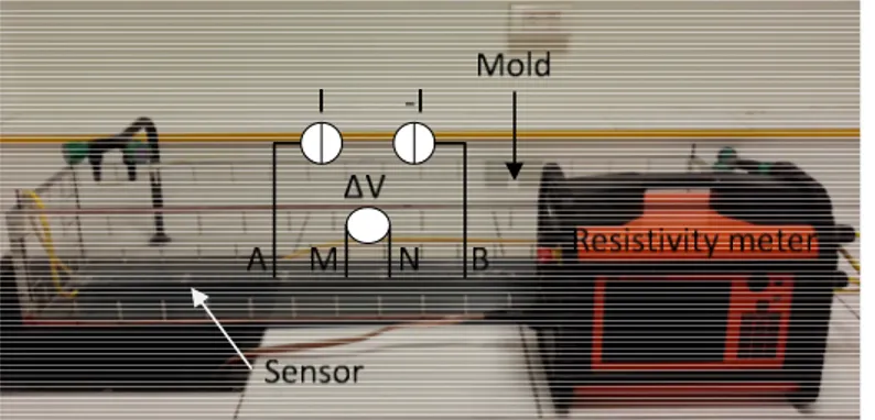
We consider the diffusion in a homogenous medium, of which the electrical resistivity is noted ρ (Ω.m), of an electrical currant I (A) injected using two surface electrodes A (injected current I) and B ( injected current -I). We measure the potential difference∆V between the electrodes M and N (see Figure 1). The expression of the resistivity is thus the following:
ρ = G∆V
I (1)
G (1/m) is the geometric factor. Assuming that the medium is infinite (case study for the soil), G depends only of the distance between electrodes. For a Wenner probe these distances are: AM = MN = NB = a, thus G = 2πa. In this experiment a (mm) is equal to 25.n (n ∈ 2;..; 14) where n is the investigation level. If the medium is not semi-infinite (case study of a concrete slab, beam, or wall) G depends also of the specimen geometry. In such a case, it has to be evaluated numerically or experimentally. Here, it has been computed thanks to a finite element simulation using the software COMSOL.
Figure 1 : Experimental device and principle of the resistivity measurement
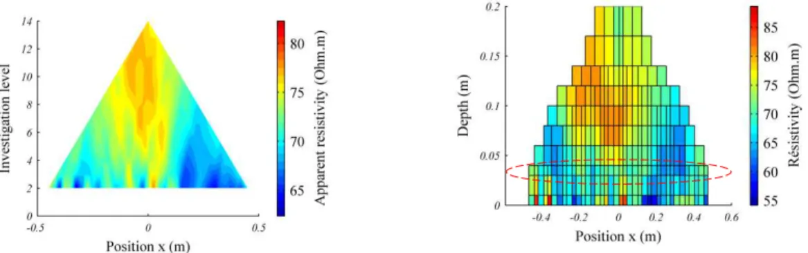
When the medium is no longer homogeneous the measured resistivities computed using the for-mula 1 are called apparent resistivities. By multiplying the number of four electrodes arrays, we obtain a pseudosection of the subsurface apparent resistivities as shown in Figure 2 a). However they are not equal to the true resistivity of the medium. It must be inverted using an optimisation protocol to find a representative model of the subsurface. After the surface potentials are measured the geometric factor
EWSHM 2014 - Nantes, France
is applied to calculate the apparent resistivity for each of the measurement point following the proce-dure described in [2]. These apparent resistivities are then inverted (using the software RES2D inv) to resolve the “true” or inverted resistivity values as a function of depth for a non-homogeneous medium. A sample of result: a section of inverted resistivity is shown in Figure 2 b).
a) Pseudo-section of apparent resistivity b) Section of inverted resistivity
Figure 2 : Sample of apparent and inverted resistivity results in concrete
1.2 Material and methods for the measurement of resistivity in concrete using an embedded sensor
The sensor used here is a PVC bar equipped with 43 electrodes spaced out at least 25mm. The bar is placed inside the mold of the beam before the concrete was poured. The beams have a section of 200 mm × 200 mm and 1170 mm in total length. The electrodes are connected to a device of soil resistivity measurement: the resistivity meter system ABEM Terrameter LS. The 43 electrodes of the sensors are tested with a Wenner sequence of measurement. In our protocol the first measurement level with electrodes spacing of 25 mm is not used. The measurement is performed starting the sequence with electrodes spacing of 50 mm (second level).
2. PERFORMANCES ASSESSMENT OF THE ACQUISITION SYSTEM(TESTS IN WATER)
Before performing tests in concrete, we have worked in a medium of known and homogenous resis-tivity in order to estimate the measurement reliability and the standard error of the entire acquisition system (sensor and Terrameter) in the absence of material uncertainties. The mold used to pour the concrete had been instrumented with the resistivity sensor and then filled with water at a constant temperature of 20◦C. The resistivity of water was controlled using a conductivity cell. Then the pseu-dosection of apparent resistivities obtained with the Terrameter allows to compute the dispersion of the resistivity values due to the acquisition system itself. We perform 10 repeatability tests for each measurement point M(xi,yi) (Figure 2 a). Three analyses are made in order to understand the origin of the measurement error and to model it.
• a) Firstly we analyze the correlation between the measurement error and the value measured, the analysis is performed for each investigation level;
• b) then, we analyze the effect of the distance to the injection electrode, the measurement error is computed for a given investigation level;
• c) finally we compute the measurement bias for each level relative to the reference value given by a conductivity probe.
For the level 2, featuring the highest number of points,for limitation of the statistical bias, we seek to analyze the correlation between the measurement error, computed as the standard deviation of
the sample containing the 10 values of the repeatability test ˜vj(xi,yi), j∈ {1;..; 10} and the magnitude
of the value measured at this point and noted ¯v(xi,yi). This one is defined as the average of the 10
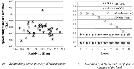
points (step a). The analysis performed here follows the guidelines issued in [5]. We plot in Figure 3 a) the scatter graph obtained for the second level of investigation which contains 37 points.
The scatter graph suggests a very fair correlation that we extrapolate to the independence between the value measured and the measurement error. It is thus possible to aggregate the errors, level by level, by centering the difference on the measuring point. We compute the standard deviation ˜vj(xi,yi) −
¯
vj(xi,yi), (i,j) ∈ {1;..; nN} × {1;..; 10} where nN is the number of measuring points for one level
(step b). It allows to reduce the statistical error since the number of measuring points for each level is given by the relationship: nN+1= nN− 3. nN takes the values 37 to 13 for the levels 2 to 10. Ten
repeatability measurements are available and the smallest sample contains 130 values. We plot on the Figure 3 b) the evolutions of the Standard Deviationσ (Ω.m) and the coefficient of variation (%) depending on the level of investigation. These values stay stable irrespective of the level with a COV of 0.26%.
For each of the ten repeatability tests, a reference value is given by the conductivity probe ˆ
vj(xi,yi), j∈ {1;..; 10}. The bias is computed using the relationship: bj,k = ˆvj− ¯vj,k where ¯vj,k is
the mean value for the level k and for the test j. The values measured using the conductivity probe are in the range from 29 to 30.77Ω.m with a mean value of 29.9 Ω.m and a standard deviation of 0.95 for the ten tests that corresponds to a CoV of 3%. The low influence of the water resistivity or temperature variation is thus taken into account.
a) Relationship error, intensity of measurement b) Evolution of σ (Ω.m) and CoV(%) as a
function of the level
0.05 0.06 0.07 0.08 0.09 0.1 0.11 0.12 28.4 28.6 28.8 29 29.2 29.4 29.6 29.8 R e p e a ta b il it y s ta n d a r d d e v ia ti o n (Ω .m ) Resitivity (Ω m) 0 0.1 0.2 0.3 0.4 0.5 0.6 0.7 0.8 0.9 1 2 3 4 5 6 7 8 9 10 Level Ecart Type CoV (%) Moy Biais ET Biais SD (Ω.m) Mean bias (Ω.m) SD bias (Ω.m)
Figure 3 : Repeatability tests performed in water
The evolution of the average bias and its standard deviation, computed using the results of ten tests, are plotted in Figure 3 b) as a function of the level. The standard deviation changes very little and is very low: in the order of 0.9Ω.m and the biais is low, staying in the range from 0.3 Ω.m to 0.75Ω.m. The CoV is therefore negligible since it is in average of 0.26 % and it always stays below 0.3 %. This confirms the importance to precisely measure a reference value using the conductivity probe for each test. Indeed the variability of the medium, estimated to be around 3 %, is above the variability measured here. Therefore, the error and the bias can be neglected. This graph allows to note an interesting property: the bias reduces significantly (by a factor of 2.5) between the level 2 and the level 10.
EWSHM 2014 - Nantes, France
Chloride content in water mixing (g/L)
Free chloride content (g/g of concrete)
Total chloride content (g/g of concrete)
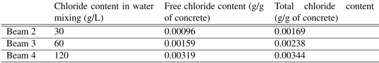
Beam 2 30 0.00096 0.00169
Beam 3 60 0.00159 0.00238
Beam 4 120 0.00319 0.00344
Table 1 : Correspondence between the free chloride content in the concrete and the initial chloride content in the mixing water
3. EVALUATION OF THE MEASUREMENT SENSITIVITY FOR THE DETECTION OF CHLORIDE
(TESTS IN CONCRETE)
In order to assess the detection threshold of chlorides, we have cast concrete beams, with different contents of chlorides, in instrumented molds. The water-cement ratio of the concrete is equal to 0.65. It is made with a Portland cement CEM I. Chloride ions were dissolved in the mixing water before the introduction in the mixer. A portion of these ions is bound to the cement paste while the remaining chlorides are free and are therefore found in pore water. These free ions are detectable using resistivity measurement. It is an interesting property for the structural health monitoring because only free ions may be able to migrate to the concrete reinforcements, locally decrease the PH, leading to the corrosion. A chloride content test was done to give the correspondence between the free chloride content in the concrete and the initial chloride content in the mixing water (c.f. Table 1).
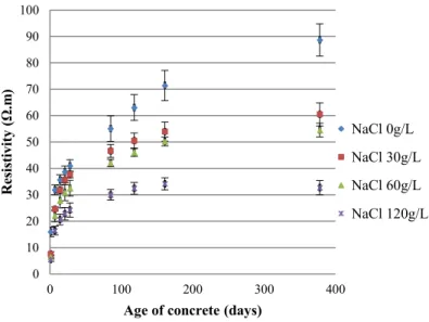
The beams instrumented with the resistivity sensors have been stored in a climatic enclosure controlled for temperature (20◦C) and relative humidity (85%). The resistivity measurements have been performed the days 1, 7, 14, 21, 28, 85, 118, 161 and 378 after pouring of concrete. The evolution of the resistivity as a function of the time for the 4 chloride contents are plotted in Figure 4. Note that the error bars depict the standard deviation of all the “true” or “inverted” resistivity values for the level 3. The material is supposed to be homogenous (mastered manufacturing processes in laboratory and phenomenon of segregation negligible at this scale). The standard deviation error for all of the resistivity values, measured in a same beam, is in the order of 10% of the mean resistivity which can be considered to be low. This curve shows a significant increase of the resistivity during the first days of the concrete life. For the first two days, the increase is related to the setting time and then the hardening of the concrete leading to a reduction of the porosity. It is the major phenomenon inducing an increase of the resistivity. At 90 days, the material has nearly reached its maximum strength. After 90 days, the water remaining not consumed by the chemical reactions starts to evaporate leading to the drying out of the porous space. With the time, the increase of resistivity becomes increasingly weak but stays significant.
3.1 Repeatability tests performed in concrete
We consider first the repeatability tests. The objective is to confirm the good repeatability highlighted with the tests in water. We conducted 5 tests for each measurement point M(xi,yi) (points on the Figure 2 a), at day 118 on the concrete beam poured without chlorides. Then we performed the same analysis as explained in the case of water for the steps a) and b). Nevertheless, in this analysis, the numerical error resulting from the inversion process appears.
We plot on the Figure 5 a) the scatter graph for the level 2. It suggests a very fair correlation between the measurement error and the mean value measured at each point. This result is the same at all levels. Consequently our hypothesis is that the measurement error is independent of the intensity of the measure. It is thus possible to aggregate the errors for each level.
We plot on the Figure 5 b) the standard deviation (Ω.m) and the COV (%) evolution as a function of the level. We notice that the standard deviation is constant and the CoV not change much. With
0 10 20 30 40 50 60 70 80 90 100 0 100 200 300 400 R es is ti v it y ( Ω .m )
Age of concrete (days)
NaCl 0g/L NaCl 30g/L NaCl 60g/L NaCl 120g/L
Figure 4 : Monitoring of the drying in a concrete made with a Portland cement CEM I (water-cement ratio = 0.65) containing different contents of chlorides in the mixing water
a COV of 0.1 %, two conclusions are inescapable: we can neglect the repeatability error and in the subsequent stages of the study, no repeatability tests are needed.
a) Relationship error, intensity of measurement b) Evolution of σ (Ω.m) and CoV(%) as a
function of the level
0 0.02 0.04 0.06 0.08 0.1 0.12 55 60 65 70 R e p e a ta b il it y s ta n d a r d d e v ia ti o n ( Ω .m ) Resistivity (Ω.m) 0 0.02 0.04 0.06 0.08 0.1 0.12 2 3 4 5 6 7 8 9 10 Level Ecart Type CoV (%) SD (Ω.m)
Figure 5 : Repeatability tests performed on concrete (without chloride in mixing water)
3.2 Evaluation of the chloride detection threshold
In order to determine the detection threshold of chlorides, we consider the study of a given measure-ment level. We focus on an intermediary level to avoid surface phenomena that are not of interest in the context of the evaluation of the chloride penetration near concrete reinforcement. An additional constraint is to have enough points to obtain a good measurement of the material variability. Thus we choose the level 3 containing 37 elements of wich the resistivity is computed during the inversion process. This level corresponds to a depth of investigation approximately equal to 35 mm (see the area circled in red on the Figure 2 b). In the context of the structural health monitoring, it could be the position of concrete reinforcements. As we can see in Figure 4, the higher the chloride level is, and the easier it is to detect chlorides with a resistivity measurement device at a given point in time. This article attempts to quantify the detection capability at a given point in time as a function of the
EWSHM 2014 - Nantes, France
chloride content. The temporal evolution allows to analyze the influence of the open porosity that de-creases over time. First of all, we will determine the optimal detection threshold and then the optimal probability of detection as a function of the chloride content at different dates. To this end, we use a probabilistic approach to define the quantities “Probability of Detection” (PoD) and “Probability of False Alarm” (PFA). We use the same definition as proposed in a previous study of void detection within tendon ducts [6]. The “noise” is here the concrete without chlorides for which no detection of chlorides should occur. We seek to detect a defect (here the presence of chloride in concrete) com-pared with a material without defects. The resistivity of a concrete without chlorides is higher than the resistivity of the same concrete containing chlorides. Thus the distribution of the signals “resistivity noise” and “resistivity signal” are reversed from the definitions usually applied [5]. The probability to detect the random defect (measured defect) ˆdand the probability of false alarm are then given by :
PoD = Z ad
−∞fSN( ˆd)∂ ˆd ; PFA =
Z ad
−∞fN(η)∂ η (2)
Where ad is the detection threshold. Below this value, no defects are detectable. fSN and fN are
respectively the probability density functions of the “signal + noise” and the “noise”. We choose to define the detection threshold using the ROC curve. It links the points of coordinates [PFA ; PoD]. Each point corresponds to measurements performed using different parameters that affect it (for ex-ample, the settings, the visibility, the operator’s experience). The curve plotted in 6 b) is obtained by continuously varying the parameter ad. According to theαδ method, we find the optimal detection
threshold that minimizes the gapδ between the corresponding point of the ROC curve and the best performance point (BPP) at coordinates [0 ; 1] (see [6]).
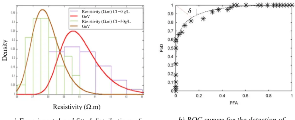
a) Experimental and fitted distributions of resistivity at 28 days
b) ROC curves for the detection of 30g/l of NaCl at 28 days. Resistivity (Ω.m) D en si ty Resistivity (Ω.m) Cl =0 g/L GeV Résistivity (Ω.m) Cl =30g/L GeV δ
Figure 6 : Evaluation of the chloride detection threshold
We plot the ROC curves and apply the method to a concrete at 28 days for the investigation level 3. To determine the detection threshold, we use the most unfavorable configuration i.e. the concrete containing 30g/l in the mixing water. The resistivity distribution for the “noise” (0g/l) and the “signal + noise”(30g/l) are plotted in Figure 6 a). In order to fit the distribution of resistivity, we have tested three classical distributions: a Normal distribution, a Generalized Extreme Values Distribution (GEV) and a Student distribution. To find the best one, we implement the maximum-likelihood method (by using the maximum of the log(likelihood) estimate (MLE)). The three parameters distribution GEV gives the best MLE and fits well the asymmetry of signal. Then we plot the experimental ROC curves (obtained by numerical integration using an increment of 0.2) and the ROC curves obtained by fitting the distributions. We observe a good agreement between the ROC curves except in the central area where the fitting of the noise distribution is not totally satisfactory (see Figure 6 a)). Then we compute the detection threshold ad corresponding to the lowest measurement δ . The line segment is plotted
in red. We thus obtained δ =0.2, and ad =37.85 Ω.m. The value ofδ , in the range [0, √
2
2 ] can be
considered low in risk analysis. The point of optimal detection has coordinates: [0.14 ; 85.5] and the probability of optimal detection is 85.5%.
CONCLUSION
In this work, we have assessed and optimized the performances of an integrated resistivity sensor compatible with Geoelectrical Imaging methods. In this way, we have performed tests in a controlled environment. Thanks to a statistical analysis of uncertainties and a probabilistic modelling we have assessed a detection threshold of chlorides in concrete. In this study, with a detection threshold of 37.85Ω.m, the probability to detect a chloride content in concrete at 28 days higher than 30g/l is 85.5%.
This work offers promising prospects on the recommendation of a detection threshold as a func-tion of time. We could also establish a unique threshold in order to optimize the SHM as a funcfunc-tion of time. Another prospect is to perform such analysis in a realistic situation i.e. with a chloride gradient in a concrete and a stochastic variability of the resistivity.
REFERENCES
[1] Polder R. B. and Peelen W. H.A. Characterisation of chloride transport and reinforcement corrosion in concrete under cyclic wetting and drying by electrical resistivity. Cement and Concrete Composites, 24(5):427 – 435, 2002.
[2] R. du Plooy, S. Palma Lopes, G. Villain, and X. Derobert. Development of a multi-ring resistivity cell and multi-electrode resistivity probe for investigation of cover concrete condition. {NDT} & E International, 54(0):27 – 36, 2013.
[3] J.F. Lataste, T. De Larrard, F. Benboudjema, and J. Semenadisse. Study of electrical resistivity: vari-ability assessment on two concretes: protocol study in laboratory and assessment on site. European Journal of Environmental and Civil Engineering, 16(3-4):298–310, 2012.
[4] F. Schoefs, J. Boero, A. Clement, and B. Capra. The alpha delta method for modelling expert judgement and combination of non-destructive testing tools in risk-based inspection context: application to marine structures. Structure and Infrastructure Engineering, 8(6):531–543, 2012.
[5] F. Schoefs, A. Clement, and A. Nouy. Assessment of{ROC} curves for inspection of random fields. Structural Safety, 31(5):409 – 419, 2009.
[6] F. Schoefs, Abraham O., and Popovics J. S. Quantitative evaluation of contactless impact echo for non-destructive assessment of void detection within tendon ducts. Construction and Building Materials, 37(0):885 – 892, 2012. Non Destructive Techniques for Assessment of Concrete.
EWSHM 2014 - Nantes, France