Antenna Physical Poles Extracted From Measured Backscattered Fields

HAL Id: hal-01394032

https://hal.archives-ouvertes.fr/hal-01394032

Submitted on 8 Nov 2016

HAL is a multi-disciplinary open access

archive for the deposit and dissemination of

sci-entific research documents, whether they are

pub-lished or not. The documents may come from

teaching and research institutions in France or

abroad, or from public or private research centers.

L’archive ouverte pluridisciplinaire HAL, est

destinée au dépôt et à la diffusion de documents

scientifiques de niveau recherche, publiés ou non,

émanant des établissements d’enseignement et de

recherche français ou étrangers, des laboratoires

publics ou privés.

Backscattered Fields

Francois Sarrazin, Philippe Pouliguen, Ala Sharaiha, Janic Chauveau, Patrick

Potier

To cite this version:

Francois Sarrazin, Philippe Pouliguen, Ala Sharaiha, Janic Chauveau, Patrick Potier.

Antenna

Physical Poles Extracted From Measured Backscattered Fields. IEEE Transactions on Antennas

and Propagation, Institute of Electrical and Electronics Engineers, 2015, 63 (9), pp.3963-3972.

�10.1109/TAP.2015.2448760�. �hal-01394032�

Abstract—This paper presents a new approach to extract the physical poles of antennas. The Singularity Expansion Method (SEM) allows modelling the antenna backscattering using poles which are theoretically independent of the wave incident angle, making them useful for antenna identification. Nevertheless, only the physical poles respect this property while the spurious poles change for each incident angle. Indeed, we call physical the poles linked to the antenna itself and spurious the poles linked to anything but the antenna (excitation, noise…). The goal of this paper is to highlight the method to define the optimal time windowing applied on the antenna backscattering in order to obtain the physical poles of the antenna. The approach is based on the Window Decreasing Technique and the Window Increasing Technique. The SEM is applied on the backscattered field measured in the boresight direction of three antennas: a narrowband patch antenna, a wideband helix antenna and a UWB antenna. By using these poles to reconstruct the field backscattered in several directions, we show that the poles extracted from one direction with this new approach are relevant to reconstruct the backscattered field for any other directions. Moreover, we show that these poles can be extracted directly from these other directions.

Index Terms—Backscattered field, antenna characterization, complex natural resonance, helix antenna, matrix pencil method, patch antenna, poles, singularity expansion method, ultra wideband antenna, window decreasing technique, window increasing technique

I. INTRODUCTION

HE Singularity Expansion Method (SEM) has been first established by C. Baum in 1971 [1]. Based on a rigorous mathematical proof, the SEM describes the global behavior of an object illuminated by an excitation wave in terms of poles, also known as complex natural resonances (CNR). The antenna backscattering due to an illuminated wave can be divided into two successive parts: the early time and the late time. While the early time response is mainly due to the excitation signal, the late time part is fully due to the internal and external resonances along the antenna. The SEM theory [1] states that only the late time response h(t) of an antenna can be modelled as a decay

This paragraph of the first footnote will contain the date on which you submitted your paper for review. This work was financially supported in part by the Direction Generale de l’Armement.

Francois Sarrazin was with the University of Rennes 1, Rennes (35042), France and is now with the Royal Military College, Kingston (K7K 7B4), Canada (e-mail: francois.sarrazin@rmc.ca).

Ala Sharaiha is with the University of Rennes 1, Rennes (35042), France (e-mail: ala.sharaiha@univ-rennes1.fr).

exponential sum as

ℎ 𝑡 ≈ .)/0𝑅)𝑒+,- (1)

where 𝑠) is the 𝑛th resonant pole, 𝑅) is the residue associated

to the 𝑛th resonant pole and 𝑁 is the number of poles of the model. Each pole is defined as 𝑠)= 𝜎)± 𝑗2𝜋𝑓), where 𝑓) is

the resonant frequency and 𝜎) is the damping coefficient.

The SEM has been first applied in the antenna domain in 1973 [2-3] and is presently still under study mainly to accurately model the antenna effective length using poles and residues [4-6]. These latter studies focus especially on reducing the amount of data needed to fully characterize an antenna. The main property of the SEM is that poles are independent of the incident wave angle as well as its polarization. Thus, it has been widely used in the radar domain to object identification such as, for example, spheres [7], aircrafts [8-9] and more recently for chipless RFID tags [10]. Indeed, poles can be interpreted as the identity card of the object which can be obtained from any incident wave angle. Practically, pole extraction leads to both spurious and physical poles. The physical poles are linked to the late time response and hence to the antenna’s behavior itself. Indeed, the currents induced on the antenna propagate along the object and then radiate back according to the antenna’s shape. However, the early time response is an entire function without poles singularities. Since a part of this early time is considered in the pole extraction process, this leads to the extraction of spurious poles. Spurious poles also include the poles due to the presence of noise and to the overestimation of the number of poles needed to fully model the late time response. In order to use these poles for identification purpose, only the physical poles have to be selected. Therefore, one has to be very careful when selecting the late time response.

The early time duration 𝑇_< is theoretically defined as 𝑇_<= 2𝐷/𝑐 + 𝑇A, where 𝐷 is the biggest dimension of the antenna, 𝑐

is the speed light and 𝑇A is the pulse duration. Nevertheless, this

computation usually leads to an overestimated 𝑇< since it

always take into account the largest dimension of the antenna, whatever the incident wave angle. Moreover, it implies that this

Philippe Pouliguen is with the Direction Generale de l’Armement (DGA), Strategy Directorate, Office for advanced research and innovation, Bagneux (92221, France (e-mail: philippe.pouliguen@intradef.gouv.fr)

Janic Chauveau and Patrick Potier are with the Direction Generale de l’Armement (DGA), Information Superiority, Bruz (35170), France, (e-mail: janic.chauveau@intradef.gouv.fr, patrick.potier@intradef.gouv.fr).

Antenna Physical Poles Extracted from

Measured Backscattered Fields

Francois Sarrazin, Philippe Pouliguen, Ala Sharaiha, Senior, IEEE, Janic Chauveau and Patrick Potier

dimension is known a priori. A common technique to define more accurately the considered window on which the SEM is applied is the Window Moving Technique (WMT) [11-13]. More recently, the Window Increasing Technique (WIT) has shown better results when dealing with noisy data [14]. Nevertheless, the end time of the window has never been studied although it impacts a lot the extracted poles. The main objective of this paper is to present a new approach to define the considered window on which the SEM is applied to extract the physical poles. This approach is based on the Window Decreasing Technique (WDT) to determine the beginning of the late time and then the WIT in order to define the window’s optimal length to avoid noise perturbation. Both techniques are based on the stability of the physical poles regarding the time window while the spurious poles vary from one window to another.

In this paper, the new approach is applied on three different antennas: a narrowband patch, a wideband helix and a UWB antenna. For each antenna, one physical set of poles is defined from the only boresight direction. Then, these poles are used to model the late time field backscattered for other incident angles. This shows the relevance of the set of poles and hence the quality of the pole extraction. Finally, the poles are directly extracted from these other directions. Indeed, in order to use these poles for antenna identification, one needs to be able to extract them directly from all directions. All the measurements have been done in the anechoic chamber CHEOPS of the Direction Générale de l’Armement, Bruz, France. This chamber is 25*25*12 m length and its Radar Cross Section (RCS) sensitivity is -60 dBm2. The measurements are done in the frequency domain in a frequency band larger than the matching bandwidth of each antenna. Then, a Gaussian shape is applied to the backscattering response before applying an Inverse Fourier Transform in order to deal with time domain data. The chamber is calibrated using a metal plate with known RCS and a specific sphere is also measured to confirm the first calibration.

Several numerical methods allow extracting poles and residues from the antenna response. In this paper, the Matrix Pencil Method (MPM) [15-16] is chosen using the Total Least Square (TLS) approach [17]. Indeed, this method offers a stronger robustness to noise than other classical extraction methods, even if the data are measured in the frequency domain [18-20]. Since the time response on which the MPM is applied is real, poles appear in complex conjugate pairs. In order to improve the readability of the figures, only the poles with positive resonant frequencies are plotted in this paper.

The section II deals with the narrow band patch antenna. The selection of the optimal window is explained in details. This includes the results of the WDT and the WIT. Then, the sections III and IV give the results for the helix antenna and the UWB antenna, respectively.

II. THE PATCH ANTENNA A. Presentation of the patch antenna

We first consider a dual polarized aperture coupled microstrip

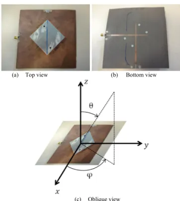
patch antenna presented in Fig. 1. There are two feeds to excite two different polarizations. In this study, only one is used and the second one is open-circuited. Each feed is composed of one microstrip line with 𝜆/4 impedance transformer to excite via a slot the 60 mm large square radiating patch. The square ground plane is 150 mm long and the distance between the ground plane and the patch is 12.5 mm. The reflection coefficient S11 is under -10 dB between 1.63 GHz and 1.92 GHz (4 % matching bandwidth). Measurements have been done between 1 GHz and 3 GHz.

B. The Window Decreasing Technique (WDT)

The measured electric far field backscattered by the patch antenna in the boresight direction (𝜃 = 0°) is presented in Fig. 2. The incident wave is polarized according to the y-axis. The first step consists in defining the beginning of the late time response. According to the theory, the early time duration is equal to 2.6 ns. To verify this value and study its impact, we suggest to use the Window Decreasing Technique (WDT). This

(a) Top view (b) Bottom view

(c) Oblique view Fig. 1. Presentation of the patch antenna.

Fig. 2. Measured electric far field backscattered by the patch antenna in the boresight direction in the time domain for a Gaussian excitation signal.

technique consists in applying the MPM on a selected window containing the whole signal (for example from 0 ns to 6 ns in Fig. 2). Then, the window’s start time is upper shifted while the window’s end time is unchanged (for example from 0.1 ns to 6 ns) and the MPM is applied again. In opposite to the classical WMT where the window’s size doesn’t change, the WDT doesn’t add new samples for each window. It avoids adding some new noisy data which disturb the pole extraction.

The WDT is applied on the patch antenna backscattered field with an end time equal to 6 ns. Results are presented in terms of resonant frequencies and damping coefficients in Fig. 3. For start time from 0 ns to 2.4 ns, poles are not completely stable, especially regarding their damping coefficients which tend to grow up in module. Then, between 2.4 ns and 4 ns, poles are very stable. Indeed, the resonant frequencies stay the same while the damping coefficients don’t vary much. Finally, for start time higher than 4 ns, poles change and become less stable. Moreover, we can see in Fig. 2 that the field is very low starting from 4 ns, it means that almost only noise is predominating in these last windows.

Thus, the WDT allows splitting this response into early time and late time parts at 2.4 ns. We notice that this value is very close to the theoretical beginning of the late time computed previously, i.e. 2.6 ns. Nevertheless, the WDT allows keeping more useful data (0.2 ns) than the classical computation of 𝑇_<.

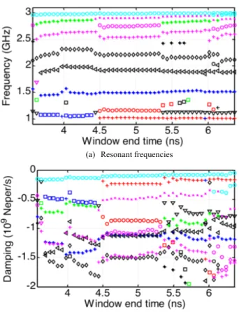
C. The Window Increasing Technique (WIT)

The Window Increasing Technique (WIT) [14] is applied to

the late time backscattered field of the patch antenna (start time _{equal to 2.4 ns). Results are presented in Fig. 4. Compared to} the WDT, the window’s start time is fixed and the window’s size increases each time. We can see that until 4.5 ns, poles are not stable. But then, between 4.5 ns and 5.3 ns, we observe a very good stability of the poles regarding both the resonant frequencies and the damping coefficients. After 5.3 ns, poles vary a lot. We can conclude that for a window’s end time smaller than 4.5 ns, the considered windows are too short to allow extracting well the CNRs. For window’s end time higher than 5.3 ns, the windows are too large and too much noisy signal is conserved. Indeed, the received signal level is very low after that time.

From these results, we conclude that the considered window is very important in order to obtain physical poles, i.e. link to the late time response only and as less disturbed as possible by the noise. Indeed, we saw that from one window to another, the poles can change a lot. For this patch antenna, the optimum window starts at 2.4 ns and end between 4.5 ns and 5.3 ns. In parts D and E, the window from 2.4 ns to 5 ns is considered to apply the MPM.

D. Physical poles extracted from the backscattered field

In addition to the window’s definition, another degree of freedom is the order 𝑁 of the SEM model, i.e. the number of poles that the MPM attends to extract from the response. The influence of 𝑁 is now studied. Poles extracted from the well-windowed backscattered field are presented in Fig. 5 in the complex plane for several 𝑁 values from 30 to 50. We can see a very good stability of the poles regarding 𝑁. Indeed, relative

(a) Resonant frequencies

(b) Damping coefficients

Fig. 3. The MPM applied on a decreasing window with a fixed end time equal to 6 ns.

(a) Resonant frequencies

(b) Damping coefficients

Fig. 4. The MPM applied on an increasing window with a fixed start time equal to 2.4 ns.

difference between those poles is under 0.5 % except for the damping coefficient of the second pole (around 1.2 GHz) where the relative difference reaches 15 %. It means that once the considered window is properly defined (using the WDT and WIT), the poles obtained using the MPM are very stable regarding the model order 𝑁.

These poles are plotted in Fig. 6 using a 𝑅 / 𝜎 weighting according to the marker’s size. This weighting highlights the most important poles. The late time field backscattered by the patch antenna can be reconstructed using these poles and (1) with a Normalized Mean Square Error (NMSE) minor than 0.001 %. Thus, a 16-poles’ set is enough to model with a high accuracy the patch antenna backscattered field.

E. Poles extracted from all directions

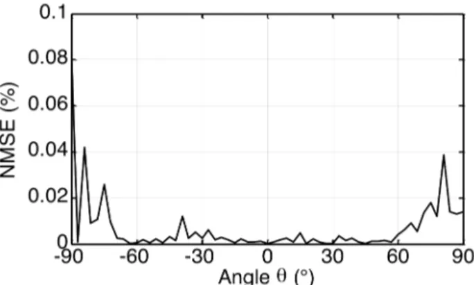
One of the main advantages of the SEM is that the poles are theoretically independent of the incident wave angle. Indeed, only the residues are different regarding the direction. This property is particularly interesting for antenna identification. The poles’ set presented in Fig. 6 has been extracted from the backscattered field in the boresight direction (𝜃 = 0°). In order to verify its validity in all the other directions, this poles’ set is used to reconstruct the field backscattered by the patch antenna in all directions of the upper half plane (𝜑 = 0°). It has to be noticed that the residues have been computed for each direction. The NMSE of the reconstructed field (using poles and residues)

as a function of the angle 𝜃 is presented in Fig. 7. We can see that the NMSE is minor than 0.02 % for all directions of incidence. Thus, the poles’ set defined in the boresight direction is very relevant for any directions.

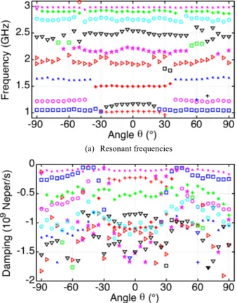
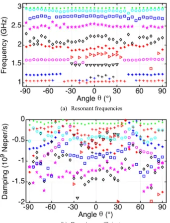
However, in order to use these poles in an identification process, one has to be able to extract this poles’ set directly from any direction. Indeed, due to the particular shape of the antenna radiation pattern, some zero radiation could appear in a particular direction and at a particular frequency. Thus, we extract poles from the field backscattered by the patch antenna in all directions of the 𝜑 = 0° plane. They are presented in terms of the resonant frequencies and the damping coefficients as a function of 𝜃 in Fig. 8.

Overall, the resonant frequencies are locally stable while the

(a) Resonant frequencies

(b) Damping coefficients

Fig. 8. Poles extracted from the measured electric far field backscattered by the patch antenna as a function of 𝜃 (𝜑 = 0° plane).

Fig. 5. Poles extracted from the windowed electric far field backscattered by the patch antenna for several N values from 30 to 50, represented in the complex plane.

Fig. 7. The Normalized Mean Square Error of the reconstructed response using the same set of poles as a function of the angle of incidence.

Fig. 6. Poles extracted from the windowed electric far field backscattered by the patch antenna, represented in the complex plane using a |𝑅|/|𝜎| weighting.

damping coefficients vary a bit from an angle to another. For −20° ≤ θ ≤ 20°, poles are very stable and close to those extracted in the boresight direction, i.e. when 𝜃 = 0°. The pole around 1.5 GHz is stable between -40° and 40°. Outside this range, another pole is extracted instead of this one. It has almost the same damping coefficient (around -1.2 109 _{Neper/s) but its}

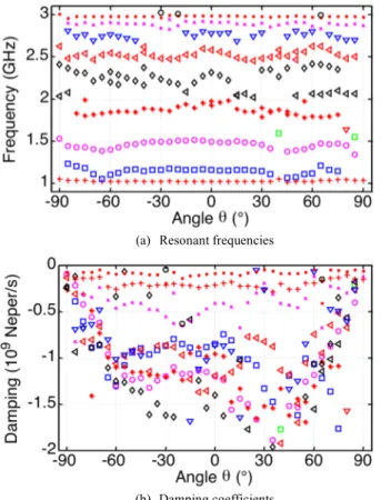
frequency is a bit higher (around 1.7 GHz). While the poles around 1.9 GHz and 2.5 GHz are almost always extracted in the same way for all angles, the resonant frequency of the pole around 2.2 GHz vary between 2 and 2.4 GHz. The same analysis is presented in Fig. 9 for the φ = 90° plane. Results are very similar to those of the φ = 0° with a good stability of the poles nearby the boresight direction (𝜃 = 0°). Nevertheless, for angles far from 𝜃 = 0°, the magnitude of the damping coefficients decrease a lot. Indeed, the level of the received backscattering in these directions (close to 𝜃 = ±90°) is very low compared to the previous case. This is due to the radiation pattern of the patch antenna. Indeed, as presented in Fig. 10 from simulation, the radiation pattern is not exactly the same in the two planes and the gain at 𝜃 = ±90° is much lower for the φ = 90° plane.

As a conclusion, the physical poles defined from the boresight direction are well extracted from other directions. This is especially true for the frequencies while the damping coefficients vary more. Moreover, the quality of the poles’ extraction can be linked to the radiation pattern of the antenna. Indeed, a zero radiation in any direction implies a very low backscattering level which disturbs a lot the poles’ extraction.

F. Poles extracted from all directions (x-axis polarized incident wave)

In this part, the poles’ independence regarding the polarization is studied. An incident wave polarized in the x-axis direction is now considered while the antenna’s position doesn’t change. Poles extracted from the field backscattered by the patch antenna in the boresight direction and illuminated by an x-axis polarized wave are presented in Fig. 11. There are two “new” poles compared to the previous polarization: around 1.6 and 2.8 GHz and the pole around 1.2 GHz is missing. Concerning the other poles, only their damping coefficients are different, especially for the main pole at 1.9 GHz. This new polarized incident wave seems to excite new different antenna modes. Thus, some new poles are extracted while some previous poles are not anymore. Indeed, all the poles are present in both polarization but their weights are so small in one of them that they cannot be extracted from measured data, i.e. noisy data. Poles extracted when the antenna is illuminated by an x-axis polarized wave are presented as a function of the θ angle for the φ = 0° plane in Fig. 12. Results are as stable as those for the y-axis polarized incident wave and are very close in terms of interpretation.

III. THE HELICAL ANTENNA A. Presentation of the helical antenna

The helical antenna studied in this part is presented in Fig. 13 [21]. A 4-turns printed helix antenna wrapped around a

(a) Resonant frequencies

(b) Damping coefficients

Fig. 9. Poles extracted from the measured electric far field backscattered by the patch antenna as a function of 𝜃 (𝜑 = 90° plane).

Fig. 11. Poles extracted using x-axis and y-axis polarized incident wave in the boresight direction, represented in the complex plane.

Fig. 10. Simulated radiation pattern of the patch antenna for two planes: φ = 0° and φ = 90° at 2 GHz.

cylindrical Rhoacell foam is placed into a truncated cone cavity with small radius equal to 58 mm and large radius equal to 120 mm. The helix is 45 mm high while the cavity is only 32 mm. This high gain antenna presents a reflection coefficient S11 minor than -10 dB between 4 GHz and 5.8 GHz, which means a 9.2 % matching bandwidth. The antenna has been measured between 3 GHz and 8 GHz.

B. Poles extracted from the backscattered field in the boresight direction

The field backscattered by the helical antenna is presented in Fig. 14 for the boresight direction (𝜃 = 0°). As for the patch antenna, the WDT is first applied in order to define the theoretical beginning of the late time. Then, the WIT is used to obtain the optimal window’s length. Finally, the MPM is applied with several 𝑁 values in order to look at the stability of the poles regarding 𝑁. This approach allows defining the optimal window between 1.2 ns and 3.2 ns. Then, the physical poles of the helical antenna are extracted using the MPM and presented in Fig. 15 with a 𝑅 / 𝜎 weighting. 12 pairs of poles are needed to model the field backscattered by the helical antenna. The NMSE of the reconstructed field using this poles’ set is minor than 0.01 % so this 24-poles’ set models with a very high accuracy the field backscattered by the antenna.

C. Poles extracted from all directions

First, we compute the NMSE of the reconstructed response using the same set of poles for each direction of the φ = 0° plane. Results are presented in Fig. 16. We observe that the

NMSE is lower than 0.1% in all directions and even lower than 0.01 % when θ is between -70° and 70°. It means that, whatever the incident wave angle, the poles’ set defined from the

Fig. 15. Poles extracted from the windowed electric far field backscattered by the helical antenna, represented in the complex plane using a |𝑅|/|𝜎| weighting.

(a) Resonant frequencies

(b) Damping coefficients

Fig. 12. Poles extracted from the measured electric far field backscattered by the patch antenna as a function of 𝜃, φ = 0°, x-axis polarized incident wave.

(a) Profile view

(b) Oblique view Fig. 13. Presentation of the helical antenna.

Fig. 14. Measured electric far field backscattered by the helical antenna in the boresight direction in the time domainfor a Gaussian excitation signal.

boresight direction is very relevant to model the backscattered field of this helical antenna.

Then, we extract poles directly from all these directions. Results are presented in terms of resonant frequencies and damping coefficients in Fig. 17. We observe that the resonant frequencies are stable even there are some slight variations, especially for angles close to 𝜃 = ±90°. The damping coefficients vary more regarding θ. Nevertheless, if we consider only the main poles (between 5 GHz and 7 GHz) most of their damping coefficients are comprised between -2 and -3 109 Neper/s whatever 𝜃. It means that they are of the same range than those extracted in the boresight direction.

IV. THE UWBANTENNA A. Presentation of the UWB antenna

The Fig. 18 presents a stripline fed printed wide-slot antenna with a fork-like tuning stub [22]. It is a 41 mm square antenna composed of two ground planes in the front and back of the stripline structure. There is a rectangular wide slot (32*21 mm) on each ground plane. Its matching bandwidth is from 2.5 GHz to 12.5 GHz, i.e. a 130 % relative bandwidth. The antenna backscattering has been measured between 2 GHz and 15 GHz.

B. Poles extracted from the backscattered field in the boresight direction

The electric far field backscattered by the UWB antenna in the boresight direction (𝜃 = 𝜑 = 90°) is presented in Fig. 19. The same approach than before is applied on the field backscattered by the UWB antenna to define the optimal window between 1.1 ns and 2.5 ns. For brevity, only the final poles’ set extracted using the MPM is presented in Fig. 20 using a 𝑅 / 𝜎 weighting.This 32-poles’ set allows modeling the backscattered field with a very good accuracy (NMSE minor than 0.01 %). This set of poles is larger than the previous ones. Indeed, the number of poles is related in part to the antenna’s bandwidth. The larger the bandwidth is, the larger the required number of poles is.

Fig. 19. Measured electric far field backscattered by the UWB antenna in the boresight direction (𝜃 = 𝜑 = 90°) in the time domain for a Gaussian excitation signal.

(a) Resonant frequencies

(b) Damping coefficients

Fig. 17. Poles extracted from the measured electric far field backscattered by the helical antenna as a function of 𝜃.

(a) Face view (b) Oblique view Fig. 18. Presentation of the UWB antenna.

Fig. 16. The Normalized Mean Square Error of the reconstructed response of the helical antenna using the same set of poles as a function of the angle of incidence θ.

C. Poles extracted from all directions

The Fig. 21 presents the NMSE of the reconstructed backscattered field for 𝜑 = 90° and 0 ≤ 𝜃 ≤ 180°. The direction 𝜃 = 90° corresponds to the boresight direction, i.e. the direction from which the poles have been extracted. We can see that the NMSE is very low (minor than 0.01 %) for 80° ≤ 𝜃 ≤ 100°, i.e. around the boresight direction and stays lower than 1 % for 30° ≤ 𝜃 ≤ 100°. Nevertheless, the NMSE increases up to 6 % for 𝜃 = 0° and more than 10 % for 𝜃 = 180° which is not negligible. We conclude that the poles’ set defined from the only boresight direction is not large enough to model completely the antenna, i.e. in all directions. Unlike the patch and the helix antenna, this antenna is an UWB. Thus, more poles are needed to completely model the antenna. Moreover, the radiation pattern could vary a lot from one frequency to another one. Therefore, since we consider only one direction, some poles can be hard to extract. Indeed, the residue associated to each pole varies according to the incident angle. It means that one pole could be significant in one direction and negligible in another one, making it impossible to extract if looking to the wrong direction. Moreover, for 𝜃 = 180°, the connector disturbs a lot the antenna’s behavior, which can explain the high NMSE for this angle.

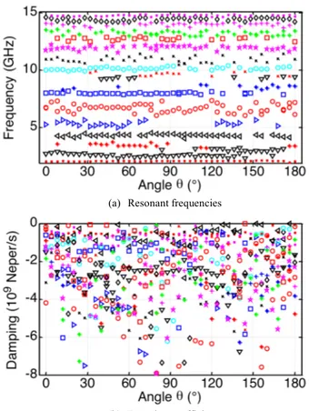
Poles extracted from fields backscattered for 𝜑 = 90° and 0 ≤ 𝜃 ≤ 180° are presented in Fig. 22. Although the damping coefficients seem to not be stable, the resonant frequencies are

quite stable, at least for 0 ≤ 𝜃 ≤ 120°. Indeed, the 8 GHz pole is almost always extracted as well as the two poles around 10 GHz. These three pairs of poles are the most significant in the boresight direction as we can see in Fig. 20. It means that the main poles can be extracted from several directions at least in terms of resonant frequencies.

Moreover, it has to be noticed that the level of the measured RCS is between -40 dBm2 _{and -60 dBm}2 _{but becomes 10 dB}

lower if only the late time response is considered (Fig. 23). This level is lower than the sensitivity of the anechoic chamber (-60 dBm2_{). The SEM is very sensitive following the antenna}

under study [23] but the pole extraction process is also very sensitive to the Signal to Noise Ratio (SNR) of the data [18]. The low SNR explains in part the poor stability of the damping

(a) Resonant frequencies

(b) Damping coefficients

Fig. 22. Poles extracted from the measured electric far field backscattered by the UWB antenna as a function of 𝜃.

Fig. 23. Measured Radar Cross Section of the UWB antenna (solid)and measured Radar Cross Section of the UWB antenna linked to the late time response only (dashed).

Fig. 20. Poles extracted from the windowed electric far field backscattered by the UWB antenna using a |𝑅|/|𝜎| weighting.

Fig. 21. The Normalized Mean Square Error of the reconstructed response of the UWB antenna using the same set of poles as a function of the angle of incidence θ.

coefficients in the UWB antenna example. However, thanks to the new poles’ selection approach presented in this paper, we saw that it is possible to obtain a very good stability of the resonant frequencies regarding the angle of incidence even for low SNR.

V. CONCLUSION

Although the SEM allows theoretically defining physical poles of an antenna which can be extracted whatever the direction, its sensitivity to the noise make this property hard to reach when dealing with antenna measurements, i.e. noisy data. In this paper, a new approach has been presented to select the optimal window on which the MPM is applied. It is based on the WDT to determine the beginning of the late time response and then the WIT allows defining the optimal window’s length. Three different antennas are considered in this paper: a narrowband patch antenna, a wideband helix antenna and a UWB antenna. First, our methodology has been applied on the measured field backscattered by these antennas in their boresight directions. This allows defining a poles’ set which model with a high accuracy the backscattered field. Then, the pertinence of these poles’ set has been studied by reconstructing the backscattered fields from other directions using always the same set of poles. For the two first antennas, the poles’ set are very relevant whatever the considered direction. Concerning the UWB antenna, some other poles have to be considered to fully model the antenna responses. Finally, the poles have been extracted directly from the field backscattered from all directions (other than boresight). The main poles are generally well extracted whatever the direction, especially regarding their resonant frequencies. As a conclusion, the new approach presented here gives very good results to obtain a physical set of poles for antennas. Nevertheless, in the case of omnidirectional antennas, more than one direction has to be considered to fully characterize them.

ACKNOWLEDGMENT

The authors thank Lilia Manac’h and Narcisse Rimbault for lending their antennas.

REFERENCES

[1] C. E. Baum, “On the singularity expansion method for the solution of electromagnetic interaction problems,” EMP Interaction Note 8, Air Force Weapons Laboratory, Kirkland AFB, New Mexico, 1971. [2] F. Tesche, “On the analysis of scattering and antenna problems using the

singularity expansion technique,” IEEE Transactions on Antennas and

Propagation,” vol. 21, no 1, pp 53-62, Jan. 1973.

[3] P. R. Barnes, “On the singularity expansion method as applied to the EMP analysis and simulation of the cylindrical dipole antenna,” EMP

Interaction Note 146, Oak Ridge National Loboratory, Tennessee, Nov.

1973.

[4] S. Licul and W. A. Davis, “Unified frequency and time-domain antenna modeling and characterization,” IEEE Transactions on Antennas and

Propagation, vol. 53, no 9, pp 2882-2888, 2005.

[5] C. Marchais, B. Uguen, A. Sharaiha, G. L. Ray and L. Le Coq, “Compact characterisation of ultrawideband antenna responses from frequency measurements,“ IET Microwaves, Antennas & Propagation, vol. 5 , Issue: 6, pp 671-675, 2011.

[6] D. Rialet, S, K. Podilchak, M. Clenet, M. Essaaidi and Y. M. M. Antar, “Characterization of compact disc monopole antennas using the singularity expansion method,” IEEE International Conference on

Wideband, pp. 412-413. Sep. 2012.

[7] W. Lee, T. K. Sarkar, H. Moon and M. Salazar-Palma, “Identification of multiple objects using their natural resonant frequencies,” IEEE Antennas

and Wireless Propagation Letter, vol. 12, pp. 54-57, 2013.

[8] C. E. Baum, E. J. Rothwell, K. M. Chen and D. P. Nyquist, “The singularity expansion method and its application to target identification,”

Proceedings of the IEEE, vol. 79, no 10, pp 1481-1492, Oct 1991.

[9] J. Chauveau, N. De Beaucoudray and J. Saillard, “Selection of contributing natural poles for the characterization of perfectly conducting targets in resonance region,” IEEE Transactions on Antennas and

Propagation, vol. 55, no 9, pp 2610-2617, Sep. 2007.

[10] A. T. Blischak and M. Manteghi, “Embedded Singularity chipless RFID tags,” IEEE Transactions on Antennas and Propagation,” vol. 59, no 11, pp 3961-3968, Nov. 2011.

[11] C. Hargrave, V. Clarkson, A. Abbosh and N. Shuley, “Radar target identification: estimating the start of the late time resonant response,”

International Conference on Radar, pp. 335-340, Sep. 2013.

[12] M. Manteghi and R. Rezaiesarlak, “Short time Matrix Pencil for chipless RFID detection applications,” IEEE Transactions on Antennas and

Propagation, 2013.

[13] S. K. Hong, W. S. Wall, T. D. Andreadis and W. A. Davis, “Practical implications of poles series convergence and the early-time in transient backscatter,” NRL Memorendum Report, Virginia Polytechnic Institute and State University, Blacksburg, Virginia, vol. NRL/MR/5740—1-9411, 2012.

[14] F. Sarrazin, P. Pouliguen, A. Sharaiha, P. Potier and J. Chauveau, “Window increasing technique to disciminate mathematical and physical resonant poles extracted from antenna response,” IET Electronic Letters, vol. 50, no 5, pp 343-344, Feb. 2014.

[15] Y. Hua and T. K. Sarkar, “Matrix pencil method for estimating parameters of exponentially damped/undamped sinusoids in noise,” IEEE

Transactions on Acoustics, Speech and Signal Processing, vol. 38, no 5,

pp 814-824, 1990.

[16] T.K. Sarkar and O. Pereira, “Using the Matrix Pencil method to estimate the parameters of a sum of complex exponentials,” IEEE Antennas and

Propagation Magazine, vol. 37, pp 45-55, Feb. 1995.

[17] S. Van Huffel, “Analysis of the total least square problem and its use in parameter estimation,” PhD. Thesis, Kattrolicke Universiterit Leuven, 1990.

[18] F. Sarrazin, J. Chauveau, P. Pouliguen, P. Potier and A. Sharaiha, “Accuracy of the singularity expansion method in time and frequency domains to characterize antennas in presence of noise,” IEEE

Transactions on Antennas and Propagation, vol. 62, no 3, pp 1261-1269,

Mar. 2014.

[19] F. Sarrazin, A. Sharaiha, P. Pouliguen, J. Chauveau and P. Potier, “Analysis of two methods of poles extraction for antenna caracterization,"

IEEE Antennas and Propagation Society International Symposium (APSURSI), pp.1,2, 2012.

[20] F. Sarrazin, A. Sharaiha, P. Pouliguen, J. Chauveau, S. Collardey and P. Potier, "Comparison between Matrix Pencil and Prony methods applied on noisy antenna responses," Loughborough Antennas and Propagation

Conference (LAPC), pp.1,4, Nov. 2011.

[21] N. Rimbault, A. Sharaiha and S. Collardey, “Low profile high gain helix antenna over a conical ground plane for UHF RFID applications,”

International Symposium on Antenna Technology and Applied Electromagnetics, pp. 1-3, 2012.

[22] C. Marchais, G. Le Ray, A. Sharaiha, “Stripline slot antenna for UWB communications,” IEEE Antennas and Wireless Propagation Letters, vol. 5, no. 1, pp. 319-322, Dec. 2006.

[23] F. Sarrazin, A. Sharaiha, P. Pouliguen, J. Chauveau and P. Potier, “Sensitivity of the singularity expansion method applied on dipole antenna backscattering,” IEEE International Symposium on Antenna

François Sarrazin was born in Poitiers,

France, in 1987. He received the M.S. degree in electronics and electrical engineering from Polytech’Nantes (Ecole

polytechnique de l’université de Nantes),

Nantes, France, in 2010. In 2013, he received the Ph.D. degree in the field of antenna characterization from RCS measurement from the Institute of Electronics and Telecommunications of Rennes (IETR), University of Rennes 1, Rennes, France. In 2014, he worked at the Royal Military College of Canada (RMCC), Kingston, Canada. He is now working at the Antenna and Propagation Laboratory of the CEA-LETI, Grenoble, France. His main research activities include antenna characterization using the Singularity Expansion Method (SEM) in both the time and spatial domains, electrically small antenna and frequency agile antenna.

Philippe Pouliguen received the M.S.

degree in signal processing and telecommunications, the Ph.D. degree in signal processing and the “Habilitation à Diriger des Recherches” degree in electronics from the University of Rennes 1, France, in 1986, 1990 and 2000. In 1990, he joined the Direction Générale de l’Armement (DGA) at the Centre d’Electronique de l’Armement (CELAR), now DGA Information Superiority (DGA/IS), in Bruz, France, where he was a “DGA expert” in electromagnetic radiation and radar signatures analysis. He was also in charge of the EMC (Expertise and ElectoMagnetism Computation) laboratory of CELAR. Since December 2009, he is the head of “acoustic and radio-electric waves” scientific domain at the office for advanced research and innovation of the strategy directorate, DGA, Bagneux, France. His research interests include electromagnetic scattering and diffraction, Radar Cross Section (RCS) measurement and modeling, asymptotic high frequency methods, radar signal processing and analysis, antenna scattering problems and Electronic Band Gap Materials. In these fields, he has published more than 30 articles in refereed journals and more than 100 conference papers.

Ala Sharaiha (SM’09)received the Ph.D. and Habilitation à Diriger la Recherche (HDR) degrees in telecommunication from the University of Rennes 1, France, in 1990 and 2001 respectively. Currently, he is a Full Professor at the University of Rennes 1, Rennes, France and the Co-Head of the ‘Complex Radiation Systems” Team in the ‘Antennas and Microwave Devices’ Department. His main research activities include small antennas, broadband and UWB antennas, reconfigurable antennas, printed spiral and helical antennas, antennas for mobile communications, etc. Conducted and involved in more than 20 industrial and collaborative projects.

Prof. Sharaiha has published more than 250 journal and conference papers, concerning antenna theory, analysis, design and measurements, and he holds 12 patents. His published

works have been cited over 500 times in Google Scholar. He has graduated/mentored over 20 Ph.D. students/post-docs,and co-authored with them.

He is presently a member of the European School of Antennas Board and a member of the small antennas working group of the European Association on Antennas and Propagation (EuRAAP). He is a senior member of the IEEE and is a reviewer for the IEEE Transactions on Antennas and Propagation, IEEE Antennas Wireless Propagation Letter, the IET Letters and the IET Microwave Antennas Propagation. He was the conference Chairman of the 11th International Canadian Conference ANTEM (Antenna Technology and Applied Electro- Magnetics), held at Saint-Malo in France, 2005.

Janic Chauveau was born in

Saint-Nazaire, France, in 1981. He received the M.S. degree in electronics and electrical engineering from Polytech’Nantes (Ecole polytechnique de l’université de Nantes), Nantes, France, in 2004. He received the Ph.D. degree in electronics from the University of Nantes, France, in 2007. He is currently working in the field of radar signatures at the Direction Générale de l’Armement (DGA), DGA-Maîtrise de l’Information, Bruz, France. His research interests include electromagnetic scattering and inverse scattering problems.

Patrick Potier received the Ph.D. degree

in structure and property of the material from the University of Rennes, Rennes, France, in 1984. From September 1984 to September 1987, he was a Research Engineer with Thomson CSF, Paris, France. Since September 1987, he has been an Engineer with the Center “Maîtrise de l’information” (Information superiority) de la “Direction Générale de l’armement” (General Armaments Directorate, the French procurement agency), Bruz, France. He treats the aspects of antennas and radiation and ensures the follow-up of various studies and theses mainly on the topics broad band reflect or transmit arrays.