Flat Gain Broad-Band Metasurface Antennas

HAL Id: hal-03099341

https://hal-univ-rennes1.archives-ouvertes.fr/hal-03099341

Submitted on 6 Jan 2021

HAL is a multi-disciplinary open access

archive for the deposit and dissemination of

sci-entific research documents, whether they are

pub-lished or not. The documents may come from

teaching and research institutions in France or

abroad, or from public or private research centers.

L’archive ouverte pluridisciplinaire HAL, est

destinée au dépôt et à la diffusion de documents

scientifiques de niveau recherche, publiés ou non,

émanant des établissements d’enseignement et de

recherche français ou étrangers, des laboratoires

publics ou privés.

To cite this version:

Marco Faenzi, David Gonzalez-Ovejero, Stefano Maci. Flat Gain Broad-Band Metasurface Antennas.

IEEE Transactions on Antennas and Propagation, Institute of Electrical and Electronics Engineers,

2021, 69 (4), pp.1942-1951. �10.1109/TAP.2020.3026476�. �hal-03099341�

Abstract—Modulated metasurface (MTS) antennas can provide a broadside pencil beam at the frequency where the cylindrical surface wave (SW) wavelength matches the period of the impedance modulation. For modulations with constant period, the mismatch between the SW wavelength and the period imposes a limitation on the gain-bandwidth product. However, this limitation can be overcome by shaping the local period as a function of the radial distance. Doing so, we generate an annular active region on the antenna aperture, where the SW-to-impedance interaction mainly occurs. Such active region moves from the antenna center to the circular rim as the frequency decreases. This paper shows that one can optimize the profile of the local periodicity function to obtain broadside pencil beams over large bandwidths, while preserving the flatness of the gain versus frequency response and a good stability of the phase center. The antenna performances so obtained are really unique for flat antennas based on printed technology. Finally, we present a simple formula for the product between average gain and bandwidth, which gradually blends into the already known expression for modulations with constant period. This formula establishes an absolute limit of the gain-bandwidth product, which only depends on the wavelength-normalized antenna radius at the central frequency.

Index Terms—Broadband antennas, circular polarization, impedance boundary conditions, leaky waves, metasurface antennas, surface waves.

I. INTRODUCTION

PERTURE ANTENNAS based on modulated

metasurfaces (MTSs) [1]-[4] have recently drawn considerable attention. Among their advantages, stand out a low weight and low profile, a relatively easy and cheap fabrication process, and a simple feeding scheme. The radiation effect in this class of antennas arises from the interaction between a surface wave (SW) and the spatially modulated tensor reactance, which transforms the bounded SW into a leaky wave (LW). By properly choosing the spatial modulation of the reactance tensor entries, one can control the

The work of M. Faenzi and D. González-Ovejero has been supported by Région Bretagne under the Stratégie d’Attractivité Durable (SAD) volet 2 programme, contract no. SAD17012, and by the European Union through the European Regional Development Fund, in part by the French Region of Brittany, Ministry of Higher Education and Research, Rennes Métropole and Conseil Départemental 35 through the CPER Project STIC & Ondes. The work of Stefano Maci has been supported by the Project of Relevant Italian Interest (PRIN) “Metasurface Antennas for Space”.

M. Faenzi and D. González-Ovejero are with Univ Rennes, CNRS, IETR (Institut d’Électronique et de Télécommunications de Rennes), UMR 6164, 35000 Rennes, France (e-mail: {marco.faenzi, david.gonzalez-ovejero}@univ-rennes1.fr).

S. Maci is with the Department of Information Engineering and

leakage rate, the direction and polarization of the radiation and even the shape of the pattern. This ability to accurately control the aperture fields has led to circular apertures that satisfy a predetermined pattern mask [5]-[7], that maximize the aperture efficiency [5],[6],[8], or that provide either dual-polarization [9],[10], multiple beams [11],[12] or dual frequency operation [13],[14].

Despite the flexibility shown by modulated MTS antennas, they have typically suffered from a relatively narrow bandwidth of gain. According to the results presented in [15], the main reason for the bandwidth limitation in modulated MTS antennas with a broadside beam is the mismatch between the periodicity d of the modulation and the dispersive variation with frequency of the SW wavelength. This variation is mostly due to the dispersion in the substrate and provokes a gradual reduction of the antenna gain at broadside.

Let us consider the case of a circular MTS antenna with radius a and with free-space wavelength λ0 at its central frequency f0. Assuming a constant period d of the impedance modulation along the radius and an optimally chosen amplitude modulation index m (see for instance [16]), the circular aperture will provide a fractional bandwidth Δf/f0=1.2(a/λ0)(vg/c), where c is the speed of light in free

space, and vg is the group velocity of the SW at f0 when it propagates on the MTS uniform average reactance. In addition, the aperture gain in absence of losses (directivity) is

G=(2πa/λ0)2(a/λ0)/(a/λ0+2) [15]. In the case of electrically large antennas, the latter expressions provide a fractional gain-bandwidth product approximately equal to 47(a/λ0)(vg/c).

Typical values of Δf/f0, where Δf is the total bandwidth, go from 9% to 3% when the gain increases from 28.5 to 40 dBi (see Fig. 5 in [15]).

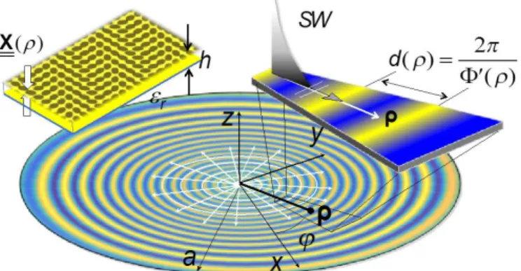
Fig. 1. Reference coordinate system and transparent reactance pattern for the broadband MTS aperture. Right inset: canonical problem of a flat SW wavefront that locally matches the modulation period. Left inset: printed elliptical elements used to implement the homogenized reactance.

Flat Gain Broad-Band Metasurface Antennas

Marco Faenzi, David Gonz

á

lez-Ovejero, Senior Member, IEEE and Stefano Maci, Fellow, IEEE

ACCEPTED MANUSCRIPT

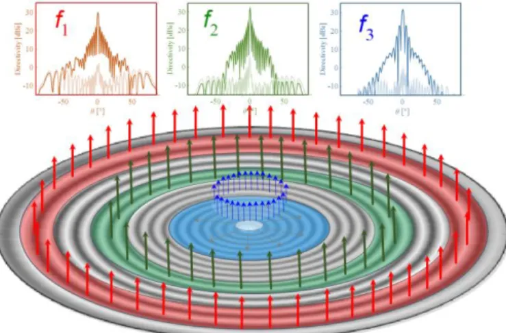
The bandwidth performance can be significantly improved by adopting a period d that changes as a function of the aperture radius [17],[18]. The period d of the modulation in [18] increases exponentially along the radial distance to match the SW wavelength in different annular regions (Fig. 1). Therefore, the designed aperture behaves as an active region antenna, where each annular region radiates the desired broadside beam at a given frequency. Increasing or decreasing the frequency implies shifting the active region towards the center or the rim of the structure, respectively. Fig. 2 illustrates the above described mechanism. It is important to note that the area outside the active region at a certain frequency barely interacts with the SW and it radiates very weakly.

Fig. 2 Active regions at three different frequencies and example of radiation patterns (f1 < f2 < f3).

Nonetheless, this exponential evolution of the period leads to a gain versus frequency response with ripples of approximately ±2 dB around its average value. Here, we show that it is possible to optimize the period function to get rid of these oscillations. Furthermore, it is seen for the first time that the phase center of these antennas is quite stable within the bandwidth. In order to reach this performance, we extend here the procedure in [18] to arbitrary period functions, optimized to have a flat gain response over a large bandwidth. To this end, we build on the technique described in [18] by introducing an accurate description of the transparent reactance, which is directly retrieved from the full-wave analysis of a local periodic canonical problem.

This paper is organized as follows. Section II presents the formulation of the problem for exponential variation of the period. Section III illustrates the design process. Section IV presents full-wave results for two different flat gain broadband apertures. Finally, conclusions are drawn in Section V.

II. EXPONENTIAL VARIATION OF THE RADIAL PERIOD We model the MTS as a sheet transition tensor impedance boundary condition (IBC) [19]. The tensor X relates the tangential electric field Et averaged at z=0 with the

discontinuity of tangential magnetic fields at the interface as

(

0 0

)

ˆ

j

t

=

 

z=+

−

z=−

E

X

z

H

H

_t (1)

where ˆz is the normal to the MTS plane.

The analyzed apertures (Fig. 1) consist of circular regions with radius a. Hence, we will use a polar coordinate system centered in the aperture at the texture layer section, with radial distance ρ, azimuth angle , and unit vectors ( ˆ ˆ, ). A generic position in the aperture is given by cosxˆ+siny and ˆ

X assumes the form [16], [18]

( )

(

( )

( )

)



( )

( )

(

)



ˆ ˆ ˆ ˆ cos ˆ ˆ ˆ ˆ sin X m m m        = +_{ }  + _   −      −  _  +   + _{ } X I (2)

where

X

_ is the average reactance, m m_, _ are the radially-dependent modulation indexes, and Φ(ρ) is the phase of the modulation given by

( )

₀ 2

_{( )}

( )

0 d d       = +  



(3)

where d(ρ) represents the local period of the modulation in ρ. We point out that, by adopting a non-uniform periodicity function d(ρ) along the radial distance, the reactance X in (2) takes the shape of a spiral that unwinds outward with a variable expansion rate that is dictated by (3).

A. Average Gain and Bandwidth

The authors treated in [18] the case m=m with an

exponential variation of the radial period of the kind

(

1

)

2

(

(

2 1

)

)

/ ( ) 1 1 a d d d e d e e      = − + −  −   (4)

where δ is a non-dimensional constant that defines the speed of the exponential growth, while d1 and d2 are the values that

the local period of the modulation assumes in ρ=0 and ρ=a; i.e., d1=d(0), d2=d a( ). The rate of growth of the exponential function depends on , which optimal value was derived in the

Appendix of [18] as . It was

shown that this choice leads to the average antenna gain ([18], eq. 28)

( )

2 ₂ min 3 2 1 4 35 2 1 ave opt a G d d a      ₋     (5)

where σmin is the ratio between the SW wavelength and the free-space wavelength at the minimum frequency of operation (occurring approximately for _sw,mind₁). The antenna bandwidth is comprised between the two frequencies for which the SW wavelength goes from the minimum value

,min 1 1

sw d

 = to the maximum value _sw,max=_{2 2}d . The factors 1,2

 are larger than one and depend on the acceptable gain (with respect to the average gain) used to define the bandwidth. For instance, these factors approach unity for a -6 dB gain bandwidth.

(a)

(b)

Fig. 3. Gain versus frequency responses for two different MTS antennas with

δ=δopt and: a) a=11.11 cm, d1=7mm and d2=13.7mm, (b) a=16.66 cm, d1=7mm

and d2=13.7mm. The peak gains and the radiation patterns in the insets have

been obtained by a full wave MoM solution for the homogenized impedance [19]. The average gain is Gave=29 dBi for a=11.11 cm with a 1dBin-band

oscillation and Gave=30 dBi for a=16.66 cm with a 2dB in-band oscillation.

Nonetheless, the choice of an exponential tapering is affected by an impairment: the gain oscillates around the average value with a ripple that increases for larger aperture radius. This undesired oscillation is related to the poor control of the aperture fields’ amplitude tapering, which is caused by the dispersivity of the surface. Fig. 3 shows two examples of broadband antenna, in both cases the substrate thickness is

h=0.635mm and the relative permittivity is εr=6.15. A

full-wave Method of Moments (MoM) solver for homogenized IBCs [19] has been used to obtain the simulation results for these antennas with radius 11.11 cm (Fig. 3(a)) and 16.66 cm (Fig. 3(b)). Both antennas have the same d1 and d2 (see the

caption in Fig. 3), and therefore the same bandwidth (22.2-29.1 GHz). Using (5), one can predict an average gain Gave=29

dBi for a=11.11 cm with 1dB in-band oscillation and Gave=30

dBi for a=16.66 cm with 2dB in-band oscillation. One can easily notice that the obtained gain is higher for the larger aperture, at the expense of larger oscillations with respect to the frequency. As expected, the side lobes exhibit higher

levels at frequencies where the gain response resents a minimum of its oscillation.

(c)

(d)

(e)

Fig. 4. (a) Fabricated prototype with an inset showing the elliptical patches used to synthesize the impedance tensor. (b) Local periodicity as a function of the radial distance. (c) Directivity versus frequency response: measured (blue line), computed with the IBC-MoM in [19] (red line), computed by CST (green line). (d) Coordinates of the phase center versus frequency calculated from measurements using the method in [20]. (e) Comparison between the z components of the phase centers calculated using the measured patterns, CST

ACCEPTED MANUSCRIPT

B. Phase Center

In some applications, the frequency stability of the phase center is an important property. The phase center (PHC) of these antennas is quite stable with frequency, since they are approximately symmetric and fed by a single monopole at the center. To illustrate this property, we have calculated the PHC for the antenna fabricated and measured in [18]. Fig. 4(a) shows the prototype and a zoom into the elliptical patches used to synthesize the IBC with the local periodicity function represented in Fig. 4(b). The PHC calculation follows the method described in [20], which is summarized here for convenience. First, the phase is obtained in the angular range of the main beam (at -3dB level). Next, the angular direction of the null of phase gradient is determined numerically. Finally, the PHC is found as the radius of the osculating spheres that match the phase gradient up to the second order derivatives around the direction of the null. It is worth noting that this procedure is different from those typically implemented in commercial softwares. In the latter, there is no search of the phase gradient null, and the osculating circle approximation is done directly on data of the main beam in a range symmetrically displaced with respect to the maximum amplitude value. This process has been found to provide significant errors in the phase center estimate even for small deviations between the maximum of the beam and the null of the phase gradient.

The variation of the PHC position with frequency is reported in Fig. 4(d), and it is obtained from measurements; Fig. 4(e) shows the z-deviation of the phase center calculated using the measured patterns, the patterns obtained from a full wave analysis in CST and those computed with the IBC-MoM in [19]. The small PHC discontinuity at 27 GHz obtained from measurements is due to a change of standard gain horn in the measurement set up. One can also observe that the phase center fluctuation is around 10 mm over the 6 GHz bandwidth.

III. ANTENNA SYNTHESIS FOR NON-EXPONENTIAL RADIAL PERIOD

One can deduct from (5) that, after setting the bandwidth, the average gain can be increased almost linearly with the radius. However, as shown in Fig. 3, when one increases the aperture size to get higher gains, the oscillation of the in-band gain becomes more pronounced. This effect is due to the insufficient control on the amplitude distribution of the “-1” indexed Floquet mode that one can get with the one-parameter () exponential periodicity function. To obtain a flat gain in frequency, we should replace the exponential period function

d(ρ) in (4) by a more general function that results from an

optimization scheme.

Fig. 5. Flow diagram for the optimization process. All the steps of this procedure are described in detail in Sections III-A to III-E. First, Section III-A presents the setup of the algorithm, namely the average gain Gave for a given

bandwidth and radius or the other way around. In section III-A, we also discuss the cost function C, the design of the periodicity function d(ρ) and the choice of the amplitude control frequency ωp. Section III-B describes the

method adopted for the evaluation of the gain based on the analytical formula (8). Section III-C illustrates the method for the design of the modulation indexes of the MTS. Finally, sections III-D and III-E provide details on the synthesis of the metasurface by metal elements and on the procedure adopted to characterize the “-1” indexed Floquet mode attenuation and propagation constants within the MTS design bandwidth.

Fig. 5 shows the flow diagram for the entire optimization process. The different steps of this process are represented by blocks in Fig. 5, these blocks are commented in the caption of Fig. 5 and described in detail in Sections III-A to III-E.

A. Optimization Scheme

As a first step, it is necessary to choose an appropriate substrate for the MTS design. We note that such choice affects the selection of the printed elements composing the MTS texture, i.e., the elliptical patches shown in Fig. 1 and Fig. 4(a). This selection allows one to fix the average transparent reactance X_ in (2) at  , which is defined as the in-band ₀ center frequency and is maintained invariant for all the iterations in the optimization process. Then, the dispersion of the wavenumber βsw is characterized for a SW propagating on the average transparent reactance X_ in the band of interest. To that end, one may adopt a constant quasi-static capacitance

0

C and a linear variation of the MTS admittance

(

0

)

1/ C

 −  [21]. This approximation can be used for the

initial choice of substrate and elements. Here, however, we use a more refined evaluation of βsw based on a full-wave periodic analysis [22].

The optimization process starts with the definition of the objective bandwidth comprised between the angular frequencies



_min and



_max, the desired average gain G_ave and the acceptable gain oscillation within the antenna bandwidth. Here, we will assume a ±1 dB of oscillation. The objective bandwidth imposes the maximum period d2 (at the periphery

X

of the aperture) and a minimum period d1 (in the feed region). The values d2 and d1 are defined to match the maximum and minimum SW wavelengths at the minimum and maximum frequencies min and, max respectively. As for the selection of

ave

G we note that such value can be approximated using the following formula , 0 0 0 28.7 g ave 28.7 ave v f a a G f c    _{ } (6)

where f0 is the antenna central frequency, λ0 is the corresponding free space wavelength, and v_{g ave,} is the integral average of the group velocity associated with X_

( )



over the bandwidth. This relation, although not relying on a rigorous basis, gradually blends into the formula given in [15]1 for modulated MTS antennas with a constant period and optimized to provide a maximum gain.

Next, one selects a set of N equally spaced frequencies fn (or

angular frequencies ωn) within the bandwidth, and associates

to each frequency the SW wavelengths values λsw,n=2π/βsw,n as

predicted from the SW dispersion curve. We will refer to ωn

as phase control frequencies. Each λsw,n is assigned to a given

value of the radial coordinate ρn so to construct the periodicity

function d(ρ). Later on, we describe the procedure followed to determine the positions ρn in the optimization algorithm. It is

important to bear in mind that just adapting the shape of the function d(ρ) will not be sufficient to get a flat frequency response. This is due to the difficulty of controlling the amplitude of the radiating “-1” indexed Floquet mode over large bandwidths. Therefore, in conjunction with the set of ρn,

it is important to choose an amplitude control frequency ωp. A

constant amplitude power distribution is imposed at ωp, which

can span over a predefined frequency range (typically the entire design bandwidth). Such frequency ωp can be changed

at each iteration within the same optimization process until an optimal value is found. The initial value of ωp is normally

selected as the in-band center frequency ω0. Further details of this process are provided in Section III-C.

At each iteration of the optimization procedure the cost function is defined as the average distance between the calculated gain G(_i) (where i are in-band equispaced

frequency samples at which the antenna gain is calculated) and the objective constant average gain Gave, namely

( ) . i ave i ave G G C G  − =



(7)

We emphasize that the gain G(_i) depends on the control frequency ωp, at which the profile of the aperture amplitude

distribution is set up as uniform (see also section III-C). In the optimization process we assume that each frequency

fn is associated with the center of the n-th active region, which

is located at the radial control point ρn. In this n-th active

1 _{We note that the formula rigorously derived in [15] has a coefficient}

different from the one in (6), 47 instead of 28.7. However, the coefficient in [15] is referred to a gain decay of -3dB, while here we refer to a +/-1 dB

region, λsw,n will match the value of the periodicity function d(ρn). Thus, the periodicity function d(ρn) is determined by

imposing d(ρn)=λsw,n. As initial guess of the optimization

procedure, we assume that the control points ρn are equispaced

along the radius. At each iteration of the optimization algorithm, both the position of the control points ρn and the

amplitude control frequency ωp are adaptively modified along

the radius and on the relevant frequency range, respectively. A swarm optimization search is used to maximize the flatness of the frequency response according to (7). We also point out that, at any iteration, the control points positions ρn do not

change their increasing order with n to ensure that d(ρ) possesses a monotonically increasing functional dependence with ρ.

In the following, the subscript n is understood and suppressed when describing the set of phase control frequencies _n, whereas we will maintain the subscript p for the amplitude control frequency ωp.

B. Calculation of Gain

To calculate the cost function according to (7), it is necessary to compute the gain as a function of the frequency at each step of the optimization process. To this end, we use the flat-optics based formula for the gain [8]

( )

(

)

(

)

2 ( , ) 2 0 2 0 , 8 , a _j a S e d G S d          _{   }  =





(8)

where S(ρ,ω) in (8) is the power density function per unit surface and

( )

0

( , )  ( )  _sw   _sw  d

 =  − −



 (9)

is the phase of the “-1” indexed modal field component of the adiabatic Floquet wave expansion [16]; Φ(ρ) in (9) represents the reactance phase provided by (3), and Δβsw accounts for an

incremental deviation of the SW wavenumber βsw due to the

reactance modulation around its average value

X

. The latter is determined as in [23] by solving the periodic canonical problem that locally matches the local period determined as explained in Section III-A (see the right inset of Fig. 1).

C. Estimate of the MTS Impedance at the Amplitude Control Frequency

The gain presents a frequency dependency due to both the aperture field power density S(ρ,ω) and the phase (,) in (9). This dependency originates from the dispersivity of the metasurface.

The in-band amplitude of the aperture fields is controlled by adaptively changing the frequency ωp. At this frequency, the

power density distribution of the “-1” indexed mode is imposed as uniform on the aperture. In particular, we enforce that S(ρ,ωp) is a uniform function with a rapid zero drop-off at

the edge and close to the source. The analytical expression of

S(ρ,ωp) is given in [18], eq.(31). From S(ρ,ωp), one can

ACCEPTED MANUSCRIPT

“-1” indexed Floquet mode as

(

)

0 ( , ) / 2 , 1 ( ', ) ' ' 2 p p sw p S P S d            = −

_

(10)

where Psw is the power associated to the SW. Such

information on α(ρ,ωp), see Fig. 5(b) in [18], combined with

the solution of a local canonical problem [23] allows one to determine the relevant modulation indexes m that best match the α(ρ,ωp) profile obtained by (10). The association between α(ρ,ωp) and m  and d(ρ) is visualized in Fig. 6.

( )

Fig.6. The colored surface represents the solution for  of the local canonical problem for several modulation indexes m and periodicity values d at the amplitude control frequency ωp. For every periodicity and its corresponding

radial distances ρn one selects the modulation index that provides the desired

α(ρn,ωp) value. All these α(ρn,ωp) are represented by the yellow dots.

The successive step consists in finding α(ρ,ω) and Δβsw(ρ,ω) as discussed in the section III-D. Finally, by using α(ρ,ω) we can compute S(ρ,ω) as a function of the frequency ω from the inversion formula of (10)

(

)

(

(

)

)

0 1 ( , ) 2 , exp 2 ', ' . 2 SW P d             = −

_

(11)

We note that by changing the control frequency _p at which S(ρ,ωp) is designed, also changes S(ρ,ω) for any other

in-band frequency.

D. Estimate of the MTS Impedance at any Frequency

In order to evaluate the functions α(ρ,ω) and Δβsw(ρ,ω) for

any ω (see the next section III-E), it is first necessary to characterize the reactance tensor X

(

ρ,ω

)

at any frequency  from the knowledge of X

(

ρ,ω_p

)

at p. To this end, the

surface is synthesized by locally periodic metallic patch elements through a database.

This element synthesis process relies on a least-square error (LSE) minimization at the amplitude control frequency ωp.

We note that to reduce the time required to synthesize the reactance tensor at each iteration, we exploit the azimuthal dependence of X in (2), which is simply linear. Therefore, the elements are designed only along the = direction, instead 0 of on the entire aperture. The reactance tensor for other values of



can then be easily recovered by straightforward algebraic relations.

After obtaining the geometry of the patches at p, we use

the in-band reactance database of the synthesized metal elements at  to determine X

(

ρ,ω

)

. This is performed by adopting a periodic MoM solver [22] that uses Rao-Wilton-Glisson (RWG) basis functions to discretize the MTS constitutive elements. The database is built up by assuming that each patch is immersed into a periodic environment constituted of identical elements arranged according to the periodic lattice. The analysis of this homogeneous structure, which is extremely fast, is repeated once for every  to construct a database that associates the entries of the anisotropic reactance tensor X

(

 

, p

)

to different angular

frequencies  and unit-cell geometries along . The extraction of the  −dependent transparent reactance tensor relevant to each element is performed using the MoM matrix with the method described in [22]. It is interesting to note that, for the particular case of the elliptical patches, this operation is carried out using the quasi-analytical formulation in [24]. To illustrate the output of this process, Fig. 7 shows the evolution of the Xρρ component of the reactance tensor X at some

frequency points within the design bandwidth.

Fig.7. The color lines represent the X component of the reactance tensor (ρ,ω)

X for different in-band frequencies ω and along the =0 direction. The X component is evaluated on a few frequency samples within the design bandwidth of the aperture.

Afterwards, by using the curves in Fig. 7 it is straightforward to reconstruct for each element (see the inset on the left of Fig. 1) the actual variation with frequency of the synthesized modulation indexes and of the average reactance

( )

X  . It is worth noting that even if the modulation indexes

ρ

m and m_φ are designed to be equal at the amplitude control frequency p (see section III-C), these two synthesized

functions mρ(ρ,ω) and mφ(ρ,ω) may slightly differ at other

frequencies .

E. In-band Relationship between Modulation Indexes and Leakage/Propagation Parameters

To complete a full iteration of the optimization loop, one should also find for every frequency  the relation between the synthesized modulation indexes mρ(ρ,ω), mφ(ρ,ω), the

leakage parameter α(ρ,ω) and Δβsw(ρ,ω). The parameters α(ρ,ω) and Δβsw(ρ,ω) represent the complex propagation

constant deviation of the “0” indexed mode with respect to the wavenumber supported by the constant (non-modulated) average transparent reactance X

( )

 .

For a given point on the aperture (0,0), such relation is obtained by using the modulation indexes mρ(ρ,ω), mφ(ρ,ω)

and the transparent reactance X

( )

 calculated in Sec. III-D

(see Fig. 7). Using these inputs, one can solve the periodic canonical problem that locally matches a modulation with: average reactance X

( )

 , modulation indexes mρ(ρ0,ω),

mφ(ρ0,ω) and period d(ρ0) [23].

The explicit formulation of this canonical problem is provided in Sec. III of [23], and constitutes a generalization for tensorial impedance of the solution found by Oliner for Leontovitch modulated scalar boundary conditions. The latter formulation is given in [25]. In the scheme of Fig. 5, the database which represents the solution of the periodic local problem is formally represented through the functional dependence

(

 

, sw

)

=FX, ,d

(

m m, 

)

. (12)

More specifically (12) represents a database of α(ρ,ω) and Δβsw(ρ,ω) for every possible impedance modulation parameter

(namely, X, ,d m m, ) at every in-band frequency .

After fixing the unit-cell size and the bandwidth of the antenna, both databases (the one for the printed elements in the band of interest and the mappings expressed by (12)) are calculated before starting the optimization process once and for all. Such information can be simply reused at any iteration of the optimization procedure at the relevant steps represented by the different blocks in Fig. 5. This renders the entire loop runtime quite fast (about 1 minute to evaluate 25 frequency samples at Ka-band for a 11.11cm radius aperture, on a 3.60 GHz I7-Intel core machine).

IV. NUMERICAL RESULTS

The optimization process described in Section III has been applied to design two broadband MTS antennas with

a=11.11cm, and characterized by the following target

bandwidth/average gains

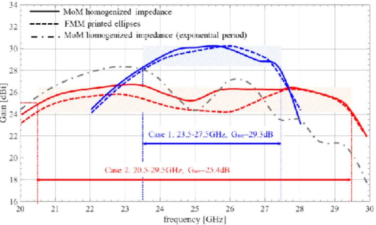
• Case 1: Bandwidth 23.5-27.5 GHz, average gain 29.3 dBi

• Case 2: Bandwidth 20.5-29.5 GHz, average gain 25.4 dBi.

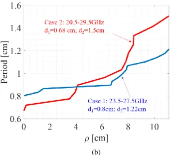
Fig. 8(a) presents the obtained gains as a function of frequency: the blue and red lines represent case 1 and case 2, respectively. On the other hand, Fig. 8(b) shows the optimized non-uniform period of the impedance modulation, with the same correspondence of colors. The solid lines in Fig. 8(a) have been obtained by using the MoM analysis in [19] to simulate the ideal IBC obtained with the optimized variables at the end of the iterative process represented in Fig. 5. This process has required about one thousand iterations in both cases for converging to the optimal solutions represented in

Fig. 8(a). The dashed lines correspond to a fast multipole method (FMM) analysis [6] of the structure synthesized by elliptical patches printed on a Rogers RO3006 substrate, with relative permittivity εr=6.15 and thickness h=0.635mm. In

both configurations, the basic square unit cell has a 1.6 mm side length. The FMM solution uses the analytical basis functions introduced in [24]. We observe that the dashed and solid lines present a good agreement and that the global response is much less oscillating than for the curves shown in Fig. 3 and Fig. 4 for an exponential variation of the radial period. The oscillation of the gain is approximately ±1 dB around an average gain of 29.3 dBi and 25.4 dBi for case 1 and case 2, respectively. Fig. 8(a) also shows a comparison between the performance of a broadband antenna designed with the proposed optimization method and a broadband antenna with an exponential variation of the periodicity function. The grey dot-dashed line in Fig. 8(a) represents the gain versus frequency response for the latter case; it has been obtained using the periodicity function in (4) with the same radius and values of d1, d2 (given in Fig. 8(b)) that characterize

case 2 introduced above. The amplitude control frequency is

fp=27GHz, as for the example in Fig. 3(a). From Fig. 8(a) it is

clear that the gain response for case 2 (red line), obtained with the optimization algorithm in Fig. 5, is considerably less oscillating around its average gain Gave. The gain response of

case 2 also features a larger bandwidth with respect to the design based on the exponential shape of the periodicity function. Besides, the peak aperture efficiency in case 1 (29% at 26 GHz, with peak directivity of 30dBi) is slightly higher than in the corresponding 11.11 cm design described in [18].

Fig. 9 presents the directivity patterns computed at various frequencies in one of the principal planes for case 1. All the sub-figures show a comparison between the co-polar components obtained with the MoM tool in [19] (solid blue lines) and with the FMM solver in [6] (dashed black lines). As for the cross-polar components, the solid green lines have been computed with the MoM analysis in [19] and the dashed red lines with the FMM solver [6]. The latter are obtained by implementing the optimized boundary conditions by printed elliptical patches.

ACCEPTED MANUSCRIPT

(b)

Fig. 8. (a) Gain versus frequency responses for the two optimized antennas with 11.11 cm radius: case 1 (blue lines) and case 2 (red lines). The solid lines stand for full-wave analysis of the homogenized impedance with the MoM tool in [19], while the dashed lines correspond to the FMM simulation [6] of the apertures synthesized by elliptical patches. The dot-dashed grey line represents the gain versus frequency response obtained for a 11.11 cm radius antenna designed by the exponential periodicity function in (4) and the same values of d1 and d2 used in case 2, and an amplitude control

frequency fp=27GHz, as in Fig. 3(a). b) Final distribution of the period as a

function of the radial distance: blue line for case 1 and red line for case 2. The agreement is excellent for both components, and shows the broadside radiation over a broad bandwidth. It is interesting to note that by tailoring the profile of d(ρ) one can also obtain dual-frequency or multi-frequency responses, topic that will be separately treated in a future work. Finally, Fig. 10 presents equivalent comparisons relevant to the case 2.

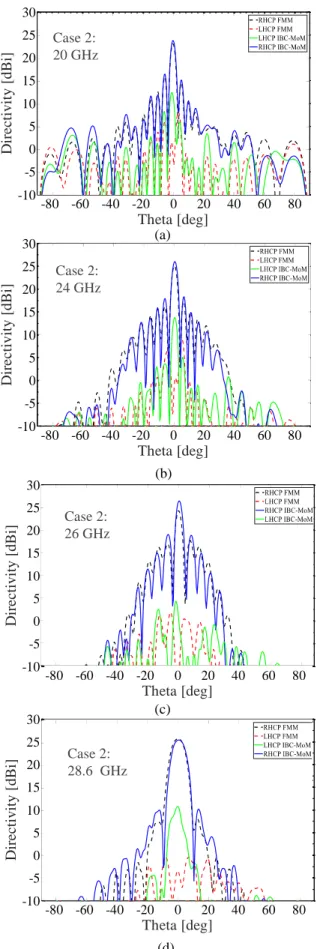
We also note that, for some frequencies, the patterns shown in Fig. 9(a) and Fig. 10(c) present side-lobe levels higher than -10dB (around -8dB). This effect is mainly due to two factors. The first one arises from the annular shape of the active regions, in particular those near the rim of the aperture (that radiate at lower frequencies within the band of interest). Indeed, the Hankel transform of an annular region with uniform amplitude presents higher side-lobe levels than a circular region with equivalent area. The second factor emerges from the radiative effect, even if weak, of the annular regions adjacent to the active one, which radiate minor beams off-broadside.

In this regard, we point out that the cost function defined in (7) for the proposed optimization algorithm includes no specific constraints on the side-lobe level. As a future research line, one may consider the control of the side-lobe level in this class of antenna. To that end, one can include specific constraints on the cost function or use different power density distribution profiles to mitigate the weak radiation coming from non-active rings.

Fig. 9. Directivity patterns for the broadband MTS in Fig. 8(a) (case 1) at (a) 23, (b) 25 and (c) 27 GHz. The blue solid lines and the green solid lines represent the RHCP and the LHCP components calculated with MoM technique in [19]. Black dashed lines and the red dashed lines represent the RHCP and the LHCP components calculated with the FMM tool in [6]. The MTS is implemented by elliptical elements, as in Fig. 4 (a).

Fig. 10. Directivity patterns for the broadband MTS in Fig. 8(a) (case 2) at (a) 20 GHz, (b) 24 GHz, (c) 26 GHz, (d) 28.6 GHz. The blue solid lines and the green solid lines represent the RHCP and the LHCP components calculated with MoM technique in [19]. Black dashed lines and red dashed lines represent the RHCP and the LHCP components calculated with the FMM tool in [6].

V. CONCLUSIONS

A design method has been presented for modulated metasurface antennas able to provide a nearly flat gain response over broad bandwidths. In one of our previous work, we adopted an exponential shape for the radial period d(ρ) of the modulated reactance, which led to a quite high oscillation of the in-band gain. In this work, we introduce an accurate formula for the gain-bandwidth product, and overcome the gain oscillations and the bandwidth limitation by optimizing the shape of the function d(ρ) and by introducing an amplitude control frequency.

On the one hand, we rely on an accurate description of the SW dispersion to optimize the periodicity function d(ρ). This function is defined by assigning to a set of radial positions periodicity values comprised between the maximum and minimum SW wavelengths at the minimum and maximum frequencies. These radial positions change at each iteration and so does the shape of d(ρ). On the other hand, we also control the amplitude of the “-1” indexed mode at each iteration. To that end, the optimization algorithm detects the optimal amplitude control frequency fp where the “-1” indexed

power density profile should be quasi-uniform. By including a variable amplitude control frequency, one obtains a more efficient illumination of the aperture rim. Therefore, it is possible to further extend the bandwidth to lower frequencies of operation. We have used the proposed technique to design two different antennas. Both designs demonstrate the possibility for trading-off bandwidth for gain without sacrificing the flatness of the frequency response. Future work will include reducing the relatively high sidelobe levels in this class of antennas.

ACKNOWLEDGMENT

The authors wish to thank Prof. Matteo Albani (University of Siena) for useful comments about the derivation of the antenna phase centers.

REFERENCES

[1] B. H. Fong, J. S. Colburn, J. J. Ottusch, J. L. Visher, and D. F. Sievenpiper, “Scalar and tensor holographic artificial impedance surfaces,” IEEE Trans. Antennas Propag., vol. 58, no. 10, 435 pp. 3212– 3221, Oct. 2010.

[2] A. M. Patel and A. Grbic, “A printed leaky-wave antenna based on a sinusoidally-modulated reactance surface,” IEEE Trans. Antennas

Propag., vol. 59, no. 6, pp. 2087–2096, Jun. 2011.

[3] G. Minatti et al., “Modulated metasurface antennas for space: Synthesis, analysis and realizations,” IEEE Trans. Antennas Propag., vol. 63, no. 4, pp. 1288–1300, Apr. 2015.

[4] D. González-Ovejero, N.Chahat, R. Sauleau, G. Chattopadhyay, S. Maci, and M. Ettorre, “Additive Manufactured Metal-Only Modulated Metasurface Antennas,” IEEE Trans. Antennas Propag., vol. 66, no. 11, pp. 6106-6114, Nov. 2018.

[5] G. Minatti, F. Caminita, E. Martini, M. Sabbadini, and S. Maci, “Synthesis of modulated-metasurface antennas with amplitude, phase, and polarization control,” IEEE Trans. Antennas Propag., vol. 64, no. 9, pp. 3907–3919, Sep. 2016.

[6] M. Faenzi et al., “Metasurface Antennas: New models, applications and realizations,” Sci. Rep., vol. 9, pp. 10178, 2019.

[7] M. Bodehou, C. Craeye, E. Martini, and I. Huynen, “A quasi-direct method for the surface impedance design of modulated metasurface antennas,” IEEE Trans. Antennas Propag., vol. 67, no. 1, pp. 24-36, Jan. 2019. -80 -60 -40 -20 0 20 40 60 80 -10 -5 0 5 10 15 20 25 30 Theta [deg] D ir e ct iv it y [ d B i] RHCP IBC-MoM LHCP IBC-MoM RHCP FMM LHCP FMM -80 -60 -40 -20 0 20 40 60 80 -10 -5 0 5 10 15 20 25 30 Theta [deg] D ir e c ti v it y [ d B i] RHCP IBC-MoM LHCP IBC-MoM RHCP FMM LHCP FMM -80 -60 -40 -20 0 20 40 60 80 -10 -5 0 5 10 15 20 25 30 Theta [deg] D ir ec ti v it y [ d B i] RHCP IBC-MoM LHCP IBC-MoM RHCP FMM LHCP FMM -80 -60 -40 -20 0 20 40 60 80 -10 -5 0 5 10 15 20 25 30 Theta [deg] D ir e ct iv it y [ d B i] RHCP IBC-MoM LHCP IBC-MoM RHCP FMM LHCP FMM Case 2: 20 GHz Case 2: 24 GHz Case 2: 26 GHz Case 2: 28.6 GHz (a) (b) (c) (d)

ACCEPTED MANUSCRIPT

[8] G. Minatti, E. Martini, and S. Maci, “Efficiency of metasurface

antennas,” IEEE Trans. Antennas Propag., vol. 65, no. 4, pp. 1532-1541, April 2017.

[9] A. T. Pereda et al., “Dual circularly polarized broadside beam metasurface antenna,” IEEE Trans. Antennas Propag., vol. 64, no. 7, pp. 2944–2953, Jul. 2016.

[10] M. Li, S. Xiao, and D. F. Sievenpiper, “Polarization-insensitive holographic surfaces with broadside radiation,” IEEE Trans. Antennas

Propag., vol. 64, no. 12, pp. 5272-5280, Dec. 2016.

[11] D. González-Ovejero, G. Minatti, G. Chattopadhyay, and S. Maci, “Multibeam by metasurface antennas,” IEEE Trans. Antennas Propag., vol. 65, no. 6, pp. 2923–2930, Jun. 2017.

[12] Y. B. Li, X. Wan, B. G. Cai, Q. Cheng, and T. J. Cui, “Frequency-controls of electromagnetic multi-beam scanning by metasurfaces,” Sci. Rep., vol. 4, Nov. 2014, Art. no. 6921.

[13] M. Faenzi, D. González-Ovejero, F. Caminita, and S. Maci, “Dual-band self-diplexed modulated metasurface antennas,” in Proc. 12nd Eur.

Conf. Antennas Propag., London, 2018.

[14] Y. Li, A. Li, T. Cui, and D. F. Sievenpiper, “Multiwavelength multiplexing hologram designed using impedance metasurfaces,” IEEE

Trans. Antennas Propag., vol. 66, no. 11, pp. 6408-6413, Nov. 2018.

[15] G. Minatti, M. Faenzi, M. Sabbadini, and S. Maci, “Bandwidth of gain in metasurface antennas,” IEEE Trans. Antennas Propag., vol. 65, no. 6, pp. 2836-2842, Jun. 2017.

[16] G. Minatti, F. Caminita, E. Martini, and S. Maci, “Flat optics for

leaky-waves on modulated metasurfaces: Adiabatic Floquet-wave

analysis,” IEEE Trans. Antennas Propag., vol. 6, no. 9, pp. 3896-3906, Sep. 2016.

[17] S. Pandi, C. A. Balanis, and C. R. Birtcher, “Analysis of Wideband Multilayered Sinusoidally Modulated Metasurface,” IEEE Antennas

Wireless Propag. Lett., vol. 15, pp. 1491-1494, 2016.

[18] M. Faenzi, D. González-Ovejero, and S. Maci, “Wideband active region metasurface antennas,” IEEE Trans. Antennas Propag., vol. 68, no. 3, pp. 1261-1272, Mar. 2020.

[19] D. González-Ovejero and S. Maci, “Gaussian ring basis functions for the analysis of modulated metasurface antennas,” IEEE Trans. Antennas

Propag., vol. 63, no. 9, pp. 3982–3993, Sep. 2015.

[20] M. Albani and S. C. Pavone, “On the (local) phase center of an antenna and its explicit derivation,” Int. Conf. Electromagn. Advanced

Applications (ICEAA), Granada, Spain, 2019, pp. 1303-1303.

[21] M. Mencagli, E. Martini, and S. Maci, “Transition function for closed-form representation of metasurface reactance,” IEEE Trans. Antennas

Propag., vol. 64, no. 1, pp. 136-145, Jan. 2016.

[22] S. Maci and A. Cucini, “FSS-based EBG surface” in Electromagnetic

Metamaterials: Physics and Engineering Aspects, N. Engheta, R.

Ziolkowski Eds., Hoboken, NJ:Wiley, 2006.

[23] F. Caminita and S. Maci, “New wine in old barrels: The use of the Oliner’s method in metasurface antenna design,” 44th Eur. Microw.

Conf., Rome, 2014.

[24] M. Mencagli, E. Martini, and S. Maci, “Surface wave dispersion for anisotropic metasurfaces constituted by elliptical patches,” IEEE Trans.

Antennas Propag., vol. 63, no. 7, pp. 2992-3003, Jul. 2015.

[25] A. Oliner and A. Hessel, “Guided waves on sinusoidally-modulated reactance surfaces,” IRE Trans. Antennas Propag., vol. 7, no. 5, pp. 201–208, Dec. 1959.

Marco Faenzi was born in Siena, Italy. He received the M.Sc. degree in telecommunications engineering and

the Ph.D. degree from the

Department of Information

Engineering and Mathematics,

University of Siena, Siena, in 2011 and 2015, respectively. In 2011, he held a Ph.D. position at the

Department of Information

Engineering and Mathematics, University of Siena, to develop high-gain modulated metasurface antennas for space. In 2018 he owned a position as Post-Doctoral Researcher with the Institut d’Électronique et de Télécommunications de Rennes, Rennes, France. Since April 2020 he is again with the

Department of Information Engineering and Mathematics at University of Siena, Siena, Italy where is currently covering a position as Post-Doctoral Researcher. His present research framework is focused on quasi-direct inversion methods for contoured beams apertures design based on modulated metasurface technology. He has worked on optimizing the aperture efficiency of metasurface holographic antennas and, during his post-doctoral appointments, toward the characterization, optimization, and synthesis of multi-band- and broadband-modulated metasurface apertures. He has also applied metasurface technology to the implementation of multibeam and high efficiency monopulse antennas with linear and circular polarizations.

Dr. Faenzi received the Sergei A. Schelkunoff Transactions Prize Paper Award from the IEEE Antennas and Propagation Society in 2016 and the Post-Doctoral Fellowship co-financed by the European Space Agency and the University of Siena in the framework of a Networking/Partnering Initiative in 2015.

David González-Ovejero (S’01– M’13–SM’17) was born in Gandía, Spain, in 1982. He received the M.S.

degree in telecommunication

engineering from the Universidad Politécnica de Valencia, Valencia, Spain, in 2005, and the Ph.D. degree in electrical engineering from the Université catholique de Louvain, Louvain-la-Neuve, Belgium, in 2012. From 2012 to 2014, he was a Research Associate with the University of Siena, Siena, Italy. In 2014, he joined the Jet Propulsion Laboratory, California Institute of Technology, Pasadena, CA, USA, where he was a Marie Curie Post-Doctoral Fellow. Since 2016, he has been a tenured researcher with the French National Center for Scientific Research, Institut d’Electronique et de Télécommunications de Rennes, Rennes, France.

Dr. González-Ovejero was a recipient of a Marie Curie International Outgoing Fellowship from the European Commission 2013, the Sergei A. Schelkunoff Transactions Prize Paper Award from the IEEE Antennas and Propagation Society in 2016, and the Best Paper Award in Antenna Design and Applications at the 11th European Conference on Antennas and Propagation in 2017. Since 2019, he has been an Associate Editor of the IEEE TRANSACTIONS ON

ANTENNAS AND PROPAGATION and the IEEE

TRANSACTIONS ON TERAHERTZ SCIENCE AND TECHNOLOGY.

Stefano Maci (M’92–SM’99–F’04) received the Laurea degree (cum laude) in electronics engineering from the University of Florence, Florence, Italy, in 1987. Since 1997, he has been a Professor with the University of Siena, Siena, Italy. In 2004, he was the Founder of the European School of Antennas, a postgraduate school that presently

comprises 30 courses on antennas, propagation, electromagnetic theory, and computational electromagnetics, with 150 teachers from 15 countries. He has coauthored over 150 articles published in international journals, among which 100 are in IEEE journals, 10 book chapters, and about 400 papers in the proceedings of international conferences. These article have received around 6700 citations. His current research interests include high-frequency and beam representation methods, computational electromagnetics, large phased arrays, planar antennas, reflector antennas and feeds, metamaterials, and metasurfaces. Prof. Maci was a recipient of the European Association on Antennas and Propagation (EurAAP) Award in 2014, the Sergei A. Schelkunoff Transactions Prize Paper Award, and the Chen-To Tai Distinguished Educator Award from the IEEE Antennas and Propagation Society (IEEE AP-S) in 2016. Since 2000, he has been a member of the Technical Advisory Board of 11 international conferences and the Review Board of 6 international journals. He has organized 25 special sessions in international conferences and held 10 short courses in the IEEE AP-S Symposia about metamaterials, antennas, and computational electromagnetics. From 2004 to 2007, he was a WP Leader of the Antenna Center of Excellence (ACE, FP6-EU), and from 2007 to 2010, he was the International Coordinator of a 24-institution consortium of the Marie Curie Action (FP6). Since 2010, he has been a Principal Investigator of six cooperative projects financed by the European Space Agency. He was the Director of the University of Siena’s Ph.D. Program in information engineering and mathematics from 2008 to 2015 and a member of the National Italian Committee for Qualification to Professor from 2013 to 2015. He is the Director of the consortium FORESEEN, which currently consists of 48 European institutions, and a Principal Investigator of the Future Emerging Technology Project Nanoarchitectronics of the 8th EU Framework Program. He was a Co-Founder of two spin-off companies. He is a Distinguished Lecturer of the IEEE AP-S and EuRAAP. He was a former Member of the IEEE AP-S AdCom, the EurAAP Board of Directors, and the Antennas and Propagation Executive Board of the Institution of Engineering and Technology, U.K. He was an Associate Editor of the IEEE TRANSACTIONS ON ANTENNAS AND PROPAGATION and the Chair of the Award Committee of IEEE AP-S.