Optimization of non destructive testing when assessing stationary stochastic processes: application to water and chloride content in concrete-Part I and II

HAL Id: hal-01008637

https://hal.archives-ouvertes.fr/hal-01008637

Submitted on 6 Feb 2018

HAL is a multi-disciplinary open access archive for the deposit and dissemination of sci-entific research documents, whether they are pub-lished or not. The documents may come from teaching and research institutions in France or abroad, or from public or private research centers.

L’archive ouverte pluridisciplinaire HAL, est destinée au dépôt et à la diffusion de documents scientifiques de niveau recherche, publiés ou non, émanant des établissements d’enseignement et de recherche français ou étrangers, des laboratoires publics ou privés.

Optimization of non destructive testing when assessing

stationary stochastic processes: application to water and

chloride content in concrete-Part I and II

Franck Schoefs, Trung-Viet Tran, Emilio Bastidas-Arteaga, Géraldine Villain,

Xavier Derobert, Alan O’Connor, Stéphanie Bonnet

To cite this version:

Franck Schoefs, Trung-Viet Tran, Emilio Bastidas-Arteaga, Géraldine Villain, Xavier Derobert, et al.. Optimization of non destructive testing when assessing stationary stochastic processes: application to water and chloride content in concrete-Part I and II. International Conference Durable Structures: from construction to rehabilitation, ICDS12, 2012, Lisboa, Portugal. �hal-01008637�

1

OPTIMIZATION OF NON DESTRUCTIVE TESTING WHEN

ASSESSING STATIONARY STOCHASTIC PROCESSES:

APPLICATION TO WATER AND CHLORIDE CONTENT IN

CONCRETE – PART1

Schoefs F. a_{, Tran T.V.}a_{, , Bastidas-Arteaga E.}a_{, Villain G.} b_{, Derobert X.} b_, O’Connor A.J.c_{, Bonnet S.} a

a_{LUNAM Université, Université de Nantes, Institute for Research in Civil and}

Mechanical Engineering, CNRS UMR 6183/FR 3473, Nantes, France; bLUNAM Université, IFSTTAR, MACS, Nantes, France; cTrinity College Dublin, Ireland

ABSTRACT

The localization of weak properties or bad behaviour of a structure is still a challenge for the improvement of Non Destructive Testing (NDT) tools. In case of random loading or material properties, this challenge is arduous because of the limited number of measures and the quasi-infinite potential positions of local failures. The paper shows that the stationary property is sufficient to find the minimum quantity of NDT measurements and their position for a given quality assessment. A measure of the quality is suggested and the illustration is performed on a one-dimensional Gaussian stochastic field for two supports: water content assessment by capacitive NDT tools and chloride ingress by semi-destructive measurements.

KEYWORDS: NDT, stochastic field, random properties, capacitive method, chloride ingress.

1 INTRODUCTION

Structural and material properties is well recognized since at least two decades to provide valuable information for: structural model updating; material property updating; monitoring of degradation and maintenance optimization; loading analysis and modelling; survey of critical quantities in the structure.

The scope of the paper takes place in this last family where a decision should be made from a set of measure of a material property (yield strength, elasticity modulus) or a mechanical quantity of interest (strain, stress) Z. In a lot of cases, the material properties are random and two

2

questions must be addressed: where is the defect and what is the probability of this event. The decision lies on a risk analysis that combines this measure of probability with the subsequent potential consequences. In practical cases, the building of large structures (soil, concrete, composite) generates a stochastic field for Z and its probabilistic properties should be used. The most simple is the stationary stochastic property. Within this context, the main objective of this work is to find the optimal geo-position of NDT measurements and their number to satisfy a given level of quality when a stationary field can describe the stochastic field and the noise of measurement should be accounting for. We suggest two illustrations in the paper part 2: a concrete beam and the water content measurement through capacitive measurements and a concrete bridge in Ireland with the semi-destructive measurement of chloride profiles.

2 PROBABILISTIC MODELING OF MEASUREMENTS IN CASE

OF SPATIAL VARIABILITY

2.1 Scope of the paper: stakes and limits

Structural health monitoring is well recognized since at least two decades to provide valuable information for:

- structural modelling updating; - material property updating;

- monitoring of degradation and maintenance optimization; - loading analysis and modelling;

- survey of critical quantities in the structure.

The scope of the paper takes place in this last family. The objective is to get a direct (so called non-model based) decision from the measurement and to detect:

- even the worst case;

- or the distribution of the worst cases (probabilistic distribution tails). The quantity of interest Z(B(x, θ),E(x, θ)) is supposed to be dependent of the hazard during building represented by the stochastic field B(x, θ) and external factors E(x, θ) where x denotes the vector of position and q is the hazard:

θ ∈ Ω

where Ω is the probabilistic space supposed to generates all the event that influence even B(x, θ) or E(x, θ). For simplicity, it is written

Z(x, θ) in the following. We note

ˆz(x,θ

i

)

one realization after measurement.

When the quantity of interest is spatially dependent and no additional information is available for characterizing the potential position of a weak region, the question is to select at which position the measurement should be done. When Non Destructing Testing tools are carried out during service

3

life, adjustments of the protocol (position, setting of the device…) can be suggested progressively with time.

When we have to design an embedded network of sensors (scope of the present paper) the choice should be the solution of an optimization problem where the quality of the data encourages increasing the number of sensors when the cost reduction tends to limit their quantity.

In this paper we consider that a solution can be obtained only if the structure of spatial variability is known. He we assume that the stochastic field is stationary (probability density function is the same whatever the location) with a known fluctuation parameter (correlation parameter) but an unknown probability density function. So we assume:

- the measured quantity can be modelled with a stationary stochastic field: as a consequence, µz and σz are constant whatever x and parameter x will be used when necessary only.

- the stochastic field is assumed to be Gaussian i.e. the considered property is normally distributed whatever the position;

- the measure is perfect in the sense that statistics moments computed from the set of

z

ˆ

(

θ

_i

)

,

i

∈

[

1

,...,

N

]

tend to the probabilistic moments of Z(θ) when N! ∞;

- a quality of the measurement can be expressed even on the form (1), (2) or (3):

Confidence interval, when the distribution of values around the mean value

is focussed on:

[

]

(

Z Z Z Z

)

z I a th z S

_p

_P

_P

_z

P

P

εµ

µ

εµ

µ

−

+

∈

=

≥

,

,ˆ

ˆ

;

ˆ , ( 1 ) where

P

_S,zˆ is the probability computed from the sensor measurements,

P

_th

the theoretical probability (implicitly non null), and pa denotes the minimum

acceptable probability to get a measurement zˆinside a given range governed by the exact value of the expectation µz and an error around this

mean value computed by the percentage ε. Note that zˆcan be replaced by its statistics like the mean value or standard deviation when statistical error (i.e. samples of small size) is investigated ([21][22]).

Distribution of extreme values, left side, when extreme low values (strength)

is analysed,

(

Z Z

)

z I a th z S

z

P

P

p

P

P

εµ

µ

−

≤

=

≤

,

,ˆ

ˆ

ˆ , (2)

4

Distribution of extreme values, right side, when extreme high values

(stress) is studied,

(

Z Z

)

z I a th z S

z

P

P

p

P

P

εµ

µ

+

≤

=

≥

,

,ˆ

ˆ

ˆ , (3)

Equations (1), (2) and (3) are compatible with a lot of numerical post-treatment algorithms for detection assessment.

Note that, at this stage no mechanical model is s-used (model free or non model based approach) and we consider a one-dimension (1D) field for illustration. Of course the methodology can be expanded to any stationary stochastic fields: 2D or 3D.

Let us assume that we get a set of independent realizations –i.e. structural components-

z

ˆ

(

θ

_i

)

of Z(θ). From a huge number of data (N≈1000),

P

S,zˆcan be estimated directly from the frequency of measurements only if it is not too small. When only a limited number of data is available (N<100), we have to assess the empirical distribution from a numerical sampling knowing the empirical distribution: it can be reached by using Monte Carlo Markov Chain. The number of components being limited the stake will be to get independent realization Ns on a given component and to consider a set

of components Nt.

Here we compute

P

_S,zˆby considering the probability density function with parameters

Z Zˆ

and

σ

ˆ

µ

computed from the empirical distribution of measurements:

( )

_∑

₍

₎

∑

= =

−

=

=

N i Z i Z N i i Z

_N

z

_N

z

1 ˆ ˆ 1 ˆ

ˆ

(

,

)

(

)

1

)

,

(

ˆ

1

)

(

x

x

θ

σ

x

x

θ

µ

x

µ

;

(4)

This variable is denoted

Zˆ

. In the following, the challenge will be to consider a model of spatial variability and to assess a set of independent realisations of Z(θ).

2.2 Spatial variability

Risk Based Inspection analysis or reliability methods applied to real structures generally assume: (i) either there is no spatial variability involved in the problem: random variables allow us to describe the hazard involved; (ii) the location of the most critical defect from reliability point of view is known and the distribution of defects in its neighbouring doesn’t affect the reliability.

5

It is well known that the reality is more complex and that we should account for stochastic fields too. Then the stochastic field could take several forms more or less complicated: (i) the most simple is the stationary stochastic field that is able to model the chloride distribution or other properties in the concrete for instance ([1],[2],[3]); (ii) more sophisticated is the piecewise stationary process that can integrate the variability of the con-creating by steps or the corrosion of structures in contiguous but different environments; (iii) finally, fully non stationary fields are certainly the most acceptable for a fine representation of properties.

However, except for natural soils, materials used for construction (airplanes, bridges …) are produced following a quality process and control. We can consider that some variation are fair, for instance the spatial change of the mean value. This paper focuses on the first model (i) only. In this paper, we used an expansion Karhunen–Loève to represent the spatial variability with this assumption of stationary ([11]):

)

(

).

(

.

.

)

,

(

1

x

x

_i n i i i Z Z

f

Z

_∑

=

+

=

µ

σ

λ

ξ

θ

θ

( 5 ) where, n is number of terms in the expansion,

_ξ

i is a set of centered

reduced Gaussian random variable (standard normal variables),

_λ

_I and

f

_i are respectively the eigenvalues and eigenfunctions of the covariance function:

ρ

( x

Δ

)

. The major interest of this representation is that

_λ

i and

f

i

have analytical expressions for specific forms of the correlation function. For instance, let us consider a one-dimensional (in space) stochastic field (x=x) with an exponential form of correlation function as follows:

0

;

exp

)

(

⎟

>

⎠

⎞

⎜

⎝

⎛ Δ

−

=

Δ

with

b

b

x

x

ρ

( 6 ) Then, it is shown that eigenvalues and eigenfunctions λI and fi have analytical expressions (7) and (8):

)

1

(

2

2 2 i

b

b

i

ω

λ

+

=

(7)

6

⎪

⎪

⎪

⎩

⎪

⎪

⎪

⎨

⎧

−

+

=

even

i

for

a

a

x

odd

i

for

a

a

x

x

f

i i i i i i i

ω

ω

ω

ω

ω

ω

.

2

)

.

.

2

sin(

)

sin(

.

2

)

.

.

2

sin(

)

cos(

)

(

(8)

where, b is lounge of correlation and ωi is solution of transcendental

equations:

⎪

⎩

⎪

⎨

⎧

=

−

=

−

even

i

for

a

b

odd

i

for

a

b

0

)

.

tan(

1

0

)

.

tan(

1

ω

ω

ω

ω

(9)

2.3 Assessment of the autocorrelation function from

measurements

We assume that the stationary stochastic field can be characterized by an autocorrelation function (ACF) considered for spatial variability of structures with their parameter, called scale of fluctuationθ. A complete overview of the auto-correlation functions and their application is available in [5]. Let us focus on the assessment of this function from experimental data (sensors or NDT tests).

Two major procedures have been reported in the literature for the estimation of δ for a spatially variable property from a digitized record of data. In the first procedure, reported by Li [4], the Maximum Likelihood Estimate method (MLE) is used in which different values for the model parameter of the proposed ACF model is assumed and the value that maximizes the corresponding MLE is taken as the model parameter. In the second procedure, proposed by Vanmarcke [7], a proposed ACF model can be adjusted to provide the best fit to the actual sample correlation coefficients ρ(Δx) thereby providing estimates of the corresponding model parameter (i.e. b in (6) and (10)).

In this paper, we select an exponential ACF (see (6)):

0

;

exp

)

(

⎟

>

⎠

⎞

⎜

⎝

⎛ Δ

−

=

Δ

with

b

b

x

x

ρ

(10)

7 ⎟ ⎟ ⎟ ⎟ ⎠ ⎞ ⎜ ⎜ ⎜ ⎜ ⎝ ⎛ − ⎟⎟ ⎠ ⎞ ⎜⎜ ⎝ ⎛ = ⎟ ⎟ ⎠ ⎞ ⎜ ⎜ ⎝ ⎛ ⎟ ⎟ ⎠ ⎞ ⎜ ⎜ ⎝ ⎛ − =

_∏

∑

= = 2 exp 2 1 2 exp 2 1 1 2 1 2 k i i k k i i L ν π ν π (11)

where νi is the ith component of the vector of independent standard values obtained from equation:

⎟⎟

⎠

⎞

⎜⎜

⎝

⎛ −

=

− Z Z

z

C

σ

µ

ν

1 (12)

where z is the vector of realizations of the random variable Z and C a lower triangular matrix such that CCT_{= ρ and ρ the autocorrelation matrix. Beside,} maximize L is equivalent to minimize L1:

∑

=

=

k i i

L

1 2 1

ν

(13)

 

8

OPTIMIZATION OF NON DESTRUCTIVE TESTING WHEN

ASSESSING STATIONARY STOCHASTIC PROCESSES:

APPLICATION TO WATER AND CHLORIDE CONTENT IN

CONCRETE – PART2

Schoefs F. a_{, Tran T.V.}a_{, , Bastidas-Arteaga E.}a_{, Villain G.} b_{, Derobert X.} b_, O’Connor A.J.c_{, Bonnet S.} a

a_{LUNAM Université, Université de Nantes, Institute for Research in Civil and}

Mechanical Engineering, CNRS UMR 6183/FR 3473, Nantes, France; bLUNAM Université, IFSTTAR, MACS, Nantes, France; cTrinity College Dublin, Ireland

ABSTRACT

The localization of weak properties or bad behaviour of a structure is still a challenge for the improvement of Non Destructive Testing (NDT) tools. In case of random loading or material properties, this challenge is arduous because of the limited number of measures and the quasi-infinite potential positions of local failures. The paper shows that the stationary property is sufficient to find the minimum quantity of NDT measurements and their position for a given quality assessment. A measure of the quality is suggested and the illustration is performed on a one-dimensional Gaussian stochastic field for two supports: water content assessment by capacitive NDT tools and chloride ingress by semi-destructive measurements.

KEYWORDS: NDT, stochastic field, random properties, capacitive method, chloride ingress.

3 OPTIMISATION OF GEO-POSITION OF SENSORS

3.1 Optimisation problem description

In this paper, we consider a one-dimensional mechanical problem with a set of sensors to be equally distributed with distance δI on Nt structures of

length L (beams of a bridge, cables, wing of an airplane, …). The optimization problem is written as a minimization problem of the number of sensors for a structure with a finite length L. In fact the question is to find the minimum number of sensors Ns in each component knowing the number

9

(

(

1

)

(

2

)

(

3

)

)

min

N

or

or

N

_S

=

_s (13)

In a complete risk analysis it can be written:

))

(

(

argmin

*

,

C

E

N

N

N

Nt Ns t S

=

=

(14)

Where E(C) denotes the expectation of the cost [19].

In this paper, we consider the optimization of position and number of inspection for two illustrations: a concrete beam and the water content measurement through capacitive measurements (IFFSTAR, France) and a concrete bridge in Ireland with the semi-destructive measurement of chloride profiles (Bridge Ferry-Carring, Ireland).

3.2 Study case 1

In this part, we consider the optimization of position and number of inspection for assessing the volume water content W (%) in a reinforced concrete beam by capacitive method (CAPA) in-site IFFSTAR, Nantes, France. Its main characteristics are 16 meters length, 1 meter height and 0.4 meter width. A grid has been drawn on each lateral surface and 2 lines of measurement have been selected: distance from the top line and the first line of measurements is 7 cm and distance between two lines is 20 cm. Distance between each measurement on one line is 20 cm.

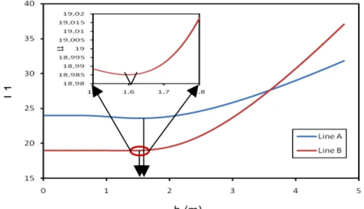
Based on measurement experimental, Fig 1 gives the same representation for the scale of fluctuation of W. The minimum values for the two exposures are 1.63 and 1.61m respectively for the line A and B. This confirms that the scale of fluctuation should be the similar because it is governed by the material properties and not for the exposure.

Herein, we focus to optimization positioning and number of captor on the RC beam when considering a stochastic stationary Gaussian field of volume water content W with its parameter µW = 10 and σW = 1.62, correlation length b = 1.62 m and the distance between two captors varied from 0.1 to 5m.

Let us consider the case with repetitive tests (i.e. without noise of measurement), and constrain [1] were ε=1(%). For a normally distributed random variable Pth=0.463 andPS,zˆ ≥0.42. Fig 2 presents this curve for

PI=42% and its fitting with a power function (red line). Based on this result, given Nt, we obtain the distance between two captors δI following [15]:

10

δ

I

=

0

.

921

( )

N

t 0.4327 [15]

and the position and minimum number of sensors are deduced. For example, for Nt=10,δI=2.2m and Ns=16/2.2 = 7.27 measure on each component, and the total number of sensor is: N=10*7=70 captors.

Fig 1: Evolution of function L1 with scale of fluctuation b of W (Data of RC beam at IFSTTAR, France)

Fig 2: The curve of Nt and δI satisfying PI =42%

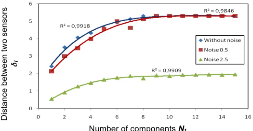
Let us considered now the absence of repetitive tests: noise of measurement exists (see Rouhan et al. 2003 for definition). Based on preliminary results (Schoefs et al. 2012) we focus study on two value of the standard deviation of a centered normally distributed with noise: 0.5 and 2.5. The later figure presents this result for the case ε=3σW = 4.68 and for PI=90% where we show the predominant role of the noise especially when it is higher than the standard deviation of the signal itself..

b (m) L1 Di st a n ce bet w een tw o se n so rs δI Number of components Nt

11

Fig 3: The curve of Nt and δI considering the noise measurement satisfying PI =90%

3.3 Study case 2

In this part, we consider the optimization of position and number of inspection for assessing the surface concentration chloride Cs in a reinforced concrete beam by semi-destructive measurement at Bridge Ferry-Carring, Ireland. Its main characteristics are 15 meters length, 1 meter height and 0.4 meter width.

The data treatment lies on a previous physical analysis to gather similar situations and distinguish others. By considering the second Fick law without initial chloride concentration (i.e. C0=0) we consider that:

- the surface chloride content CS depends on the environment and

two exposures are considered: for each beam: north and south. For the structure considered in [20], Fig 4 shows the evolution of L1 with

scale of fluctuation b for Cs and two minimum values of this function are

obtained for the two exposures: 0.7 and 1.9m respectively for the North and the South exposures.

Herein, we focus to optimization positioning and number of captor at zone North on the RC beam when considering a stochastic stationary Gaussian field of volume water content W with its parameter µCs = 19.61E-4 and σCs = 4.82E-4, correlation length b = 0.7 m and the distance between two captors varied from 0.1 to 5m.

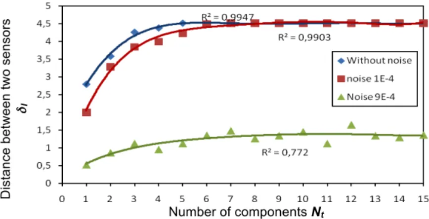
Based on preliminary results (Schoefs et al. 2012) we focus study on two value of the standard deviation of a centered normally distributed with noise: 1E-4 and 9E-4. The later figure presents this result for the case ε=3σW = 14.46E-4 and for PI=90% where we show the predominant role of the noise especially when it is higher than the standard deviation of the signal itself in the Fig 5.

Di st a n ce bet w een tw o se n so rs δI Number of components Nt

12

Fig 4: Evolution of function L1 with scale of fluctuation b of CS (Data of

Bridge Ferry-Carring, Ireland)

Fig 5: The curve of Nt and δI considering the noise measurement satisfying PI =90%

4 CONCLUSIONS

This papers aim to focus on the first step of a work dealing with uncertainty in measure assessment and intrinsic spatial variability. Only the case of stationary Gaussian fields of properties is investigated herein. It is shown how to model a stationary stochastic field and to follow up this property to get a good representation of a random variable from a limited number of NDT measurements. We developed an illustration based on capacitive and semi- destructive measurements with and without error of measurements.

Di st a n ce bet w een tw o se n so rs δI Number of components Nt

13

This result can be exploited in further reliability updating once the first measurements are available.

ACKNOWLEDGEMENTS

The authors would like to thank the ECND-PdL project (project about Condition Assessment, Monitoring and Non Destructive in the Pays de la Loire region) to support this project. Contact: Franck.Schoefs@univ-nantes.fr.

.

REFERENCES

[1] BAZANT Z. P., NOVÁK D., “Probabilistic Nonlocal Theory for Quasibrittle Fracture Initiation and Size Effect. I: Theory”, Journal of

Engineering Mechanics. 2000a ,Vol. 126, No. 2, 166-174.”

[2] BAZANT Z. P., NOVÁK D., Probabilistic Nonlocal Theory for Quasibrittle Fracture Initiation and Size Effect. II: Application”, Journal

of Engineering Mechanics, 2000b. Vol. 126, No. 2, 175-185.

[3] BAZANT Z. P., XI Y., “Statistical Size Effect in Quasi-brittle Structures: II. Nonlocal Theory”, ASCE J. of Engrg. Mech. 1991, Vol. 117, No. 11, 2623-2640.

[4] FABER M.H., “Risk Based Inspection: The Framework”. Structural

Engineering International (SEI), 12(3), August 2002, pp. 186-194.

[5] GOMES, H. M., and AWRUCH, A. M., “Reliability of reinforced concrete structures using stochastic finite elements”, Engineering Computations, 2002, 19(7-8), 764- 786.

[6] KENSHEL O.M., “Influence of spatial variability on whole life management of reinforced concrete”. PhD Thesis, University of Dublin, Trinity College, August 2009.

[7] LI, Y., “Effect of spatial variability on maintenance and repair decisions for concrete structures”, PhD thesis, Delft University, Delft, Netherlands. 2004

[8] MARK G.S., and ALI AL-HARTHY., “Pitting corrosion and structural reliability of corroding RC structures: Experimental data and probabilistic analysis”. Rreliability Engineering and System Safety, 2008, 93, 373-382.

[9] ROUHAN, A., SCHOEFS, F. Probabilistic modelling of inspections results for offshore structures. Structural Safety, Vol. 25, 2003, pp. 379-399.

[10] SCHOEFS F., TRAN T.V., BASTIDAS-ARTEAGA E., “Optimization of inspection and monitoring of structures in case of spatial fields of

14

deterioration/properties”. Applications of Statistics and Probability in

Civil Engineering, Taylor & Francis Group, London, ISBN

978-0-415-66986-3. 2011c

[11] SCHOEFS F., BOÉRO J., CLÉMENT A., CAPRA B., “The ad method for modeling expert Judgment and combination of NDT tools in RBI context : application to Marine Structures”. Structure and

Infrastructure Engineering: Maintenance, Management, Life-Cycle Design and performance (NSIE), Special Issue “Monitoring, Modeling and Assessment of Structural Deterioration in Marine Environments”,

accepted January 2010, Vol. 8, N° 6, April 2012, pp. 531-543, doi: 10.1080/15732479.2010.505374.

[12] YUAN X.-X, PANDEY M.D., “Analysis of approximations for multinormale integration in system reliability computation”, Structural

Safety, 2006, 28, 361-377.

[13] SØRENSEN J.D. and FABER M.H., “Codified Risk-Based Inspection Planning”. Structural Engineering International (SEI), 12(3), August 2002, pp. 195-199.

[14] SCHOEFS F., YÁÑEZ-GODOY H., Lanata F., “Polynomial Chaos Representation for Identification of Mechanical Characteristics of Instrumented Structures: Application to a Pile Supported Wharf”.

Computer Aided Civil And Infrastructure Engineering, spec. Issue “Structural Health Monitoring”,Volume 26, Issue 3, pages 173–189,

April 2011b.

[15] SCHOEFS F., CLÉMENT A., NOUY A., “Assessment of spatially dependent ROC curves for inspection of random fields of defects”.Structural Safety, Vol. 31, Issue 5, September 2009, pp. 409-419

[16] SCHOEFS F., “Risk analysis of structures in presence of stochastic fields of deterioration: coupling of inspection and structural reliability”.

Australian Journal of Structural Engineering, Special Issue “Disaster & Hazard Mitigation”, 2009, Vol. 9, N°1, pp. 67-78.

[17] SCHOEFS F., TRAN T.V., E. BASTIDAS-ARTEAGA., “Optimization of inspection and monitoring of structures in case of spatial fields of deterioration/properties”. 10th International Conference on Applications of Statistics and Probability in Civil Engineering – ICASP 2011, Switzerland, August 1-4, 2011a

[18] STEWART M.G., and Al-HARTHY A., “Pitting corrosion and structural reliability of corroding RC structures: Experimental data and probabilistic analysis”. Reliability Engineering and System Safety, 2008, 93, 373-382.

[19] STRAUB, D., FABER, M.H., “Modelling dependency in inspection performance”, Proc. Application of Statistics and Probability in Civil Engineering, ICASP 2003 – San Franncisco, Der Kiureghian, Madanat and Pestana eds., Mill-press, Rotterdam, ISBN 90 5966 004 8. pp. 1123-1130.

15

[20] TRAN T.V., SCHOEFS F., BASTIDAS-ARTEAGA E., VILLAIN G., DEROBERT X., “Optimization of NDT measurements for structural reliability assessment in case of spatial variability”, International Workshop « Non Destructive Testing and Evaluation: Physics, Sensors, Materials and Information », November 21-22 2011, Ecole Centrale de Nantes, France.

[21] TRAN T.V., BASTIDAS-ARTEAGA E., SCHOEFS F., BONNET S., O’CONNOR A.J., and LANATA F. “Structural reliability analysis of deteriorating RC bridges considering spatial variability”. 6th International Conference on Bridge Maintenance, Safety and Managements – IABMAS 2012, Italy, July 8-12, 2012a.

[22] TRAN T.V., SCHOEFS F., BASTIDAS-ARTEAGA E., VILLAIN G., DEROBERT X., “Optimization Of Geo-positioning Of Sensors In Case Of Spatial Fields Of Deterioration/Properties”, EACS 2012 – 5th

European Conference on Structural Control , paper #212, 11 pages, Genoa, Italy – 18-20 June 2012, 2012b.

[23] VANMARCKE, E., “Random fields: analysis and synthesis”, MIT Press, Cambridge, Mass; London. 1983.

[24] VANMARCKE, E., and GRIGORIU, M., “Stochastic Finite Element Analysis of Simple Beams”. Journal of Engineering Mechanics, 1983, 109(5), 1203-1214.

View publication stats View publication stats