Auteurs:
Authors: Moussa Djioua et Réjean Plamondon
Date: 2008
Type: Rapport / Report
Référence:
Citation:
Djioua, M. & Plamondon, R. (2008). A new algorithm and system for the
extraction of delta-lognormal parameters (Rapport technique n°
EPM–RT–2008-04).
Document en libre accès dans PolyPublie
Open Access document in PolyPublie
URL de PolyPublie:
PolyPublie URL: https://publications.polymtl.ca/3165/
Version: Version officielle de l'éditeur / Published versionNon révisé par les pairs / Unrefereed
Conditions d’utilisation:
Terms of Use: Tous droits réservés / All rights reserved
Document publié chez l’éditeur officiel
Document issued by the official publisher
Maison d’édition:
Publisher: Les Éditions de l’École Polytechnique
URL officiel:
Official URL: https://publications.polymtl.ca/3165/
Mention légale:
Legal notice: Tous droits réservés / All rights reserved
Ce fichier a été téléchargé à partir de PolyPublie, le dépôt institutionnel de Polytechnique Montréal
This file has been downloaded from PolyPublie, the institutional repository of Polytechnique Montréal
A NEW ALGORITHM AND SYSTEM FOR THE EXTRACTION OF DELTA-LOGNORMAL PARAMETERS
Moussa Djioua et Réjean Plamondon Département de Génie électrique
Laboratoire Scribens École Polytechnique de Montréal
EPM-RT-2008-04
A New Algorithm and System for the Extraction of
Delta-Lognormal Parameters
Moussa DJIOUA et Réjean PLAMONDON
Département de Génie Électrique,
Laboratoire Scribens,
École Polytechnique de Montréal.
Moussa Djioua, Réjean Plamondon
Tous droits réservés Bibliothèque nationale du Québec, 2008 Bibliothèque nationale du Canada, 2008 EPM-RT-2008-04
A New Algorithm and System for the Extraction of Delta-Lognormal Parameters : Moussa Djioua, Réjean Plamondon
Département de génie électrique, Laboratoire Scribens École Polytechnique de Montréal
Toute reproduction de ce document à des fins d'étude personnelle ou de recherche est autorisée à la condition que la citation ci-dessus y soit mentionnée.
Tout autre usage doit faire l'objet d'une autorisation écrite des auteurs. Les demandes peuvent être adressées directement aux auteurs (consulter le bottin sur le site http://www.polymtl.ca/) ou par l'entremise de la Bibliothèque :
École Polytechnique de Montréal
Bibliothèque – Service de fourniture de documents Case postale 6079, Succursale «Centre-Ville» Montréal (Québec)
Canada H3C 3A7
Téléphone : (514) 340-4846
Télécopie : (514) 340-4026
Courrier électronique : [email protected]
Ce rapport technique peut-être repéré par auteur et par titre dans le catalogue de la Bibliothèque : http://www.polymtl.ca/biblio/catalogue/
3
-Abstract—In this report, we present a new analytical method to estimate the parameters of
Delta-lognormal functions. According to the Kinematic Theory of rapid human movements, these parameters contain information both on the motor commands and on the timing properties of a neuromuscular system. The new algorithm, called XZERO, exploits relationships between the zero crossings of the first and the second time-derivatives of a lognormal function and its four basic parameters. The methodology is described and evaluated in various testing conditions. Furthermore, for the first time, the extraction accuracy is quantified empirically, taking advantage of the exponential relationships that link the disperssion of the extraction errors with its signal to noise ratio. A new extraction system, which uses a benchmark of three estimation methods, is also proposed and evaluated in the mid-term perspective of developing machine intelligence applications that rely on lognormal functions.
Index Terms— Pattern recognition, Kinematic Theory, rapid movement, Delta-Lognormal
model, lognormal function, parameter extraction, motor control, nonlinear regression, optimization, curve fitting.
—————————— ——————————
1 INTRODUCTION
I
N pattern analysis and recognition of on-line handwriting, various methods use a disconti-nuous representation scheme to represent a complex pattern, like a graph, a letter, a word, a signature, etc., with the superimposition of handwriting strokes, considered as a specific class of rapid human movements [1],[2],[3],[4],[5]. In motor control, these strokes are considered as primitives from which, complex movements are build[6],[7],[8],[9],[10], [11],[12]. Thus, handwriting strokes have been intensively used and studied in many fields of research.
For example, in the forensic sciences, a detailed study of individual stroke patterns, fo-cusing on tiny variations, often constitutes the grounds for a decision about the authen-ticity of a signature or a document [13],[14]. In education, various interactive teaching methods have been developed to reproduce letters and words from the concatenation of neat strokes [15], [16]. In the neurosciences, strokes are analyzed to both characterize neuro-degenerative processes like Parkinson’s and Alzheimer’s diseases [17],[18] and, to eva-luate the recovery processes in the rehabilitation of patients from cerebrovascular acci-dents [19]. In anthropomorphic robotics, the superimposition of handwriting strokes is used to explore the biomechanical principles employed by humans to produce movements and later to apply them in the control of a robot arm [20].
Many of these examples suggest that for a realistic analysis and understanding of how the motor control system performs complex movements, one should study the basic properties of single strokes. Running such a study for a specific application, one could then use a segmen-tation/superimposition strategy to construct an efficient machine intelligent system, which could globally processes complex movements to design for example an online handwriting recognition system [1]. The cornerstone of this whole methodology is then to understand, in the first place, the stroke genesis, since it reflects some fundamental properties of the neu-romuscular system of a writer, as well as some basic features of the motor control strat-egies that are used to produce a simple movement. In this perspective, many studies have been conducted to understand the emergence of a basic pattern: the stereotyped bell-shaped velocity profile of these basic primitives [21],[22],[23],[24]. Among the various
-computational models and theories developed to model this phenomenon, the Kinematic Theory [25] exploits an analytical expression, a Delta-Lognormal function, which takes into account the behavior of agonist and antagonist lognormal neuromuscular systems, specified by four system parameters, and describes the effective motor control of a movement by three command parameters. So far, many applications based on this theory have been developed [26],[27],[28],[35]. However, in term of fully automatic pattern analysis, the quest for an effi-cient software tool (an extraction system), which accurately estimates the seven parameters such that a velocity profile can be fitted with a Delta-Lognormal equation with a minimum reconstruction error remains an open problem. Consequently, various methods have been proposed to track this task, leading to three main categories of approaches: statistical, deter-ministic and evolutionary. Statistical methods rely on parameter estimation algorithms that deal with lognormal random variable densities [29], [30]. Deterministic methods focus on specific points on the velocity curve to first estimate the parameters and then use optimization algorithms to converge on optimal solutions [31],[32]. Evolutionary methods, using for ex-ample breeder genetic algorithms, have also been implemented [33], [34], [35].
Moreover, comparative studies have shown that the deterministic methods were more effi-cient than the statistical [27] and the evolutionary ones [33],[34]. So far, two deterministic approaches have lead to successful applications dealing with the analysis-by-synthesis of handwriting and signature verification [26],[27],[28],[31],[35], as well as the quantification of the performances of the Delta-Lognormal model with more than 26 other kinematic mod-els [36],[37],[38],[39]. However, some studies have shown that these deterministic algo-rithms fail especially when the antagonist component is preponderant before the agonist component and when important noise is present in the signal [32],[40].
-In this paper, we propose a new analytical algorithm developed to compensate for these vari-ous failures, to improve the performances of the existing extraction system, and to enlarge the range of Delta-Lognormal profiles that can be processed automatically. In summary, the new algorithm exploits analytical expressions that link the zero crossing of the first and the second time-derivatives of a lognormal function to its parameters. Furthermore, this study includes a methodology to quantify the accuracy of the extraction results under noise constraints by constructing a confidence interval for each extracted parameter value.
The remaining of the paper is organized as follows: In section 2, an overview of the Kinemat-ic Theory and its Delta-Lognormal model is presented, while the architecture of the extrac-tion system is depicted in Secextrac-tion 3. The new XZERO algorithm is described in details in Section 4. The performance results obtained in ideal and noisy conditions are presented and discussed in Section 5. In Section 6, a complete extraction system is proposed and the metho-dology used to quantify its accuracy is developed. Typical examples involving real data are presented in section 7 to highlight the power of the upgraded Delta-Lognormal extraction system.
2
OVERVIEW OF THE DELTA-
LOGNORMAL MODELAmong the various models used to study rapid movements, the Delta-Lognormal model has been found over the years to be one of the most powerful in its capability to reconstruct, with a minimum of errors, the velocity profile of handwritten strokes [25],[26],[41],[42]. This model is the kernel of the Kinematic Theory of Rapid Human Movements, initially proposed in the context of handwriting [25], [41] and later extended to process other bio-signals [2],[40]. This Theory describes the velocity profile of an end-effector by a Delta-Lognormal equation:
-( )
(
2)
(
)
1 ; , ,0 1 1 2 ; , ,0 2 2 v t =DΛ t t μ σ −DΛ t t μ σ2 (1) where,(
)
(
)
(
)
2 0 2 2 0 0 1 exp 1 ln for 2 2 ; , , 0 e t t t t t t t t μ σ σ π σ μ ⎧ ⎧ ⎡ ⎤ ⎫ 0 lsewhere − − − > ⎨ ⎬ ⎪ − ⎣ ⎦ Λ =⎨ ⎩ ⎭ ⎪ ⎩ (2) and, 1, 2D D : the amplitudes of the input commands. Their effects correspond to the distances cov-ered by the individual agonist (1) and antagonist (2) components.
0
t : the time occurrence of the input commands, a time-shift parameter. 1, 2
μ μ : the logtime delays, the time delays of the neuromuscular systems expressed on a logarithmic time scale. Explicitly, eμrepresents the median of a lognormal profile.
1, 2
σ σ : the logresponse times, the response times of the neuromuscular systems expressed on a logarithmic time scale.
According to this representation, a rapid movement, produced by an end-effector, is the result of a synergy made up of an agonist and an antagonist neuromuscular systems. Each neuromuscular system is modeled by the convolution product of an infinite number of coupled subsystems and its corresponding impulse response converges toward a lognormal function. These impulse responses, once convolved with the input commands, represent re-spectively the agonist and the antagonist components of the velocity profile, which can be described synthetically by the seven parameters
(
t D0, , , , , ,1 μ σ1 1 D2 μ σ of the Delta-2 2)
Lognormal pattern.-3 O
UTLINES OF THE DELTA-
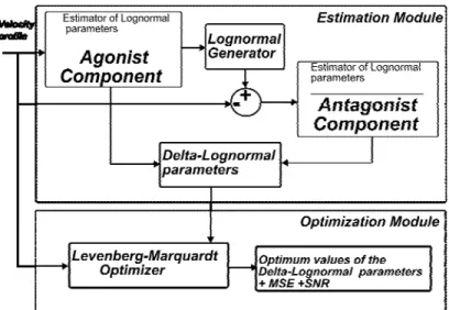
LOGNORMAL EXTRACTORThe functioning of the Delta-Lognormal extractor is schematised in Figure 1. Given a typical velocity profile , the algorithm first estimates the agonist lognormal parame-ters by considering as a single lognormal profile. Then, the antagonist lognormal profile is deduct by subtracting the agonist lognormal profile from the velocity. The second step consists in the estimation of the antagonist lognormal parameters. Then, the estimated values of the seven parameters serve as a starting solution for an optimizing algorithm. Indeed, these initial estimated values may represent only a coarse solution de-pending on the experimental conditions under which handwriting data was collected. Starting from these coarse solutions, the extractor seeks for optimized values using a mean square nonlinear regression technique that minimizes the distance between experi-mental data and the predicted Delta-Lognormal model [43].
( )
v t
( )
v t
At the end of the process, one can obtain both the optimal values of the seven parameters and the mean square reconstruction error (MSE) between the original and the recon-structed velocity profiles.
Fig 1: General architecture of the Delta-Lognormal extraction system
4.
T
HEXZERO
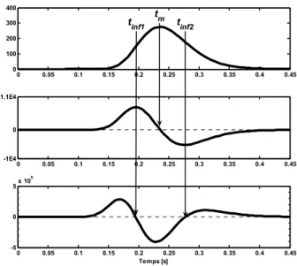
ALGORITHMThe previous architecture has been exploited by other algorithms in the past [31],[32] and it has been shown that its critical path was the initial estimation process: the better the starting solutions, the better the optimization results. Our new algorithm proposes an original solution to this estimation process; it exploits the analytical relationships that ex-ist between three specific time-indexes of a lognormal profile Λ
( )
t (a maximum and two inflexion points) and its four parameters. As illustrated in Figure 2, the time occurrence of the maximum corresponds to the solution of d t dtΛ( )
=0 and the time occurrences of the inflexion points correspond respectively to the solutions of d2Λ( )
t dt2 =0. For this reason, the new algorithm has been named XZERO, referring to these zero crossings. .-0 0.05 0.1 0.15 0.2 0.25 0.3 0.35 0.4 0.45 0 100 200 300 400 0 0.05 0.1 0.15 0.2 0.25 0.3 0.35 0.4 0.45 -1E4 0 1.1E4 0 0.05 0.1 0.15 0.2 0.25 0.3 0.35 0.4 0.45 -5 0 5x 10 5 Temps [s] tm tinf1 tinf2
Fig 2. Illustration of a lognormal function and its first and second time-derivatives to highlight the time-indexes of the maximum and the inflexion points.
4.1. Estimation of lognormal parameters
The estimation of single lognormal parameters consists in linking the experimental val-ues of these zero crossings to their corresponding analytical expressions.
Let consider
(
2)
0; , ,
v t t μ σ be a lognormal function weighted by and shifted by : D t0
(
)
(
)
( ) ( ) 2 0 2 ln 2 2 2 0 0 0 0 , ; , , ; , , 2 0 elsewere t t D e t v t t D t t t t μ σ μ σ μ σ σ π ⎡ − − ⎤ ⎣ ⎦ − ⎧ ⎪ > ⎪ = Λ = ⎨ − ⎪ ⎪⎩ t (3)(
2)
( )
(
)
22 0 0 ; , , , 2 k D v t t v t k e t t μ σ σ π − = = − (4) where(
)
(
)
0 0 ln t t dk 1 k dt t t μ σ σ − − = → = − 10-The first lognormal derivative is given by: ( ) ( ) ( ) (( )) ( ) 2 2 0 0 ; ; ; 2 k dv t k v t k d D e v t k k dt dt σ t t π σ t t σ − ⎡ ⎤ = = ⎢ ⎥= − − − ⎢ ⎥ ⎣ ⎦ & + (5)
where and are respectively the first and the second time-derivative of a function . The non-trivial zeros of this function occur when
v& v&&
( )
v t σ+ =k 0v.g.:(
0)
2 0 ln 0 m t t k kμ
t t eμ σσ
σ
σ
− − − + = → = = − → = +The time occurrence of the maximum that corresponds to this zero crossing is given by: 2
0
m
t
= +
t e
μ σ−(6)
Similarly, the second time-derivative of the shifted and weighted lognormal function is:
( )
(
)
( )
( ) ( )
( )
(
)
(
)
2 2 0 2 2 2 2 0 ; ; ; ; 3 2 1 d v t k v t k d v t k dt dt t t v t k k k t t σ σ σ σ σ ⎛ + ⎞ = = ⎜⎜− − ⎟⎟ ⎝ ⎠ k = + + − − && (7)The zeros of this function are calculated by solving the following equation:
2 3 2 2 1
k + σk+ σ − =0 (8) 11
-Let k1,2 3 2 2
σ σ
− ± +
= 4 be the two solutions Then, the roots are given by:
2 2 inf 1 0 exp 3 2 4 0 1 t = +t ⎪⎧μ σ− ⎜⎛ σ+ σ + ⎟⎞⎪⎫= +t αeμ σ− ⎨ ⎜ ⎟⎬ ⎪ ⎝ ⎠⎪ ⎩ ⎭ (9.a) 2 2 inf 2 0 exp 3 2 4 0 2 t = +t ⎪⎧μ σ− ⎜⎛ σ− σ + ⎟⎞⎪⎫= +t αeμ σ− ⎨ ⎜ ⎟⎬ ⎪ ⎝ ⎠⎪ ⎩ ⎭ (9.b) with 1 2 1 2 4 0 1 a a =σ⎧⎪σ+ σ + ⎫⎪> →α = − ⎨ ⎬ ⎪ ⎪ ⎩ ⎭ e <1 (10.a) 2 2 2 2 4 0 2 a a =σ⎧⎪σ− σ + ⎫⎪< →α = − ⎨ ⎬ ⎪ ⎪ ⎩ ⎭ e >1 (10.b) and inf 1 m inf 2 t < t <t (11) In practice, these three time indexes are calculated from sampled velocity profiles by considering the time occurrences of the maximum velocity to estimate and the time occurrences of the maximum and the minimum of the acceleration to estimate and
respectively. m t inf 1 t inf 2 t
Thus, by using (6), (9.a) and (9.b) one can express t D0, ,μandσ as a function of and . inf 1 , m t t tinf 2 12
-4.1.1 Estimation of σ
The parameter σ is estimated by solving a non-linear equation. Indeed, let consider the interval I , which covers 99.97% of the surface under a lognormal curve:
[
]
3 3 min max , , I =⎡eμ σ− eμ σ+ ⎤= t t ⎣ ⎦ (12)where and are the extreme bounds of the interval, as estimated from the log-normal profile using empirical thresholds (v.g. the times when the velocity reaches 1% of its maximum). Then:
min t tmax
(
)
3 3 3 3 max min eμ σ+ −eμ σ− =e eμ σ −e−σ t −t (13)( )
max min 2sinh 3 t t eμ σ − (14) 2 3 min m t −t e eμ⎡ −σ −e−σ⎤ ⎣ ⎦ (15)and finally, σ is evaluated by solving the following nonlinear relationship:
( ) max ( )min 2 3 ( ) min 0 2sinh 3t t m F σ eσ e σ t σ − − t − ⎡ ⎤ = ⎣ − ⎦− − = (16)
4.1.2. Estimation of the other parameters
Using the estimated value σ ofσ , the estimated value ˆˆ μ of μ can be computed by:
-(
)
(
)
2 2 2 1 ˆ ˆ ˆ ˆ ˆ ˆ inf 2 inf1 a a ˆ2 ˆ1 t −t =eμ σ− e− −e− = α α− eμ−σ (17) 2 inf 2 inf 1 2 1 ˆ ˆ ln t ˆ tˆ μ σ α α ⎛ − ⎞ = + ⎜ − ⎝ ⎠⎟ (18)with α et ˆ1 α the estimated values of ˆ2 α and1 α .Then one can estimate : 2 t0
ˆ ˆ2 0 ˆ m t = −t eμ σ− (19) and D, using:
( )
(
)
( ) ( )2 0 2 1 ln ˆ ˆ ˆ 2 m 0 ˆ ˆ 2 m t t m m D v t v e t t μ σ σ π − − − = = − (20) ( ) 2 2 2 2 2 1 ˆ ˆ ˆ ˆ ˆ ˆ 2 2 m ˆ ˆ ˆ ˆ 2 2 D D v e e e σ μ σ μ μ σ μ σ σ π σ π − − − − + − = = (21) 2 ˆ ˆ 2 m ˆ ˆ 2 D v= σ πeμ−σ (22) where is the maximum velocity. vm4.2. Estimation of the Delta-Lognormal parameters
The estimation of the agonist lognormal parameters is performed by exploiting directly the above method since a Delta-Lognormal profile is given by:
( )
1( )
2( )
v t =v t v t− (23)
-where and are respectively the agonist and the antagonist components. Us-ing (16) to (22), the agonist parameters are estimated by considerUs-ing the main peak of the velocity profile as a single lognormal function (
( )
1
v t v t2
( )
( )
1( )
, inf 1 inf 2v t ≈v t t < <t t ). The antagonist parameters are then evaluated after subtracting the agonist
componentv t1
( )
. From the total velocity profilev t( )
. The time indexes of the resulting lognormal functionv t2( )
are given by:2 2 2 2 0 m t = +t eμ σ− (24) 2 2 2 1 inf 12 0 a t = +t eμ σ− e− (25) 2 2 2 2 inf 22 0 a t = +t eμ σ− e− (26)
The following expressions are then used to estimate σ : 2
2 2 2 2 1 2 2 2 2 1 inf 22 0 inf 12 0 a a a a t t e e e t t e e μ σ μ σ − − − − − − = = − (27) Considering inf 22 0 1 2 inf 12 0 ln t t B a a t t ⎛ − ⎞ = − = ⎜ − ⎝ ⎠⎟, a positive constant: inf 22 0 inf 22 0 inf 12 inf 22 inf 12 0 inf12 0 1 t t 0 ln t t t t B t t t t ⎛ − < → < → < = ⎜ − ⎝ − ⎠ ⎞ − ⎟ (28) 2
(
2) (
2 2)
1 2 2 2 2 4 2 2 2 4 a a− − =B σ σ + σ + −σ σ − σ + − =B 0 (29) then(
)
2 2 2 2 4 B2 σ σ + = (30) 15Using 2 2
l=σ , equation (30) becomes a second order polynomial:
l2+ −4l B2 =0 (31) The parameter σ is calculated from the positive solution of (31): 2
2 2
ˆ B 4 2
σ = + − (32) The estimated value μˆ2 of the parameter μ2is computed by the following expression:
2 inf 22 inf 12 2 2 ln t At μ =σ + ⎢⎡ − ⎤⎥ ⎣ ⎦ (33) with $22 $12 a a A e= − −e− (34) and finally, the estimated value of is given by: ˆD2 D2
2 2 0.5 22
2
2max 2
D =v σ πeμ − σ (35)
where v2maxis the maximum value of v t2
( )
.5.
T
ESTING UNDER IDEAL CONDITIONSAfter implementing XZERO on a software benchmark, a testing phase under ideal con-ditions has been performed. It consisted in building an ideal database of Delta-Lognormal functions, and comparing the performances of our new algorithm with two previously developed deterministic algorithms: INFLEX [31] and INITRI [32]. INFLEX uses a graphical method for the initial estimation, based on the characteristics of the tangents of the inflexion points of the main velocity peak, while INITRI uses analytical relationships
-between the parameters and the time occurrence of the maximum velocity and two other arbitrary points located in the rising phase of the velocity curve.
5.1. Construction of the database
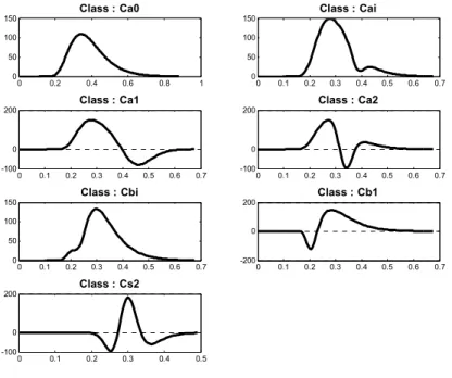
Theoretically, one can generate an infinite number of velocity profiles from the super-position of two agonist and antagonist lognormal components. The construction of our database aimed at grouping this large variety into a few classes. To reach this goal, two main features were considered to classify the ideal profiles into seven classes (i) the number of zero crossings appearing in the velocity profile, and (ii) the position of the antagonist component with respect to the agonist one [40]. Figure 3 depicts typical exam-ples for each class Cuw, where the subscript u indicates where the dominance of the
anta-gonist component occurs with respect to the antaanta-gonist one (b : before, a: after or s:
si-multaneous) and the subscript w represents the number of zero crossings 0, 1 or 2. The
label i (imaginary) is used when there is no real roots to the zero crossing equation
[32],[41]. As one can see in these plots, the different timings of the antagonist versus the agonist curves generate a large variety of primitive patterns.
-0 0.2 0.4 0.6 0.8 1 0 50 100 150 Class : Ca0 0 0.1 0.2 0.3 0.4 0.5 0.6 0.7 0 50 100 150 Class : Cai 0 0.1 0.2 0.3 0.4 0.5 0.6 0.7 -100 0 200 Class : Ca1 0 0.1 0.2 0.3 0.4 0.5 0.6 0.7 -100 0 200 Class : Ca2 0 0.1 0.2 0.3 0.4 0.5 0.6 0.7 0 50 100 150 Class : Cbi 0 0.1 0.2 0.3 0.4 0.5 0.6 0.7 -200 0 200 Class : Cb1 0 0.1 0.2 0.3 0.4 0.5 -100 0 200 Class : Cs2
Fig 3. The seven classes of Delta-Lognormal velocity profiles as generated by a synergy of an artificial agonist and antagonist neuromuscular systems.
This wide variability is obtained by randomly selecting the Delta-Lognormal parameter values within specific intervals, these intervals being fixed according to typical features of rapid movements. In this data base, we assumed that the movement time was typically between 100 ms and 500 ms, and the minimum time occurrence of the maximum about 100 ms, as measured from . The lower bound of this latter parameter was fixed consi-dering the fact that a human being does not respond without anticipation to a stimulus faster than 50 ms. The upper bound was arbitrary fixed at one second. The parameters and were empirically deduct by taking into account both the dimension of the digitizer used to acquire real data (31cmx23 cm) and the assumption that the distance covered by the antagonist movement was smaller than the one covered by the agonist.
0
t
1
D D2
-The corresponding ratio was fixed to D2max ≈0.1D1maxto emulate worst-case testing con-ditions [34] (see Table 1).
TABLE 1.VARIATION RANGES OF THE DELTA
-LOGNORMAL PARAMETERS [34]
Parameters Min Max 0(s) t 0.05 1.0 5 70 2(cm) D 0.5 7 1, 2 μ μ -2.2 -1.6 1, 2 σ σ 0.1 0.45 5.2. Performance evaluation
To test our algorithm, each ideal Delta-Lognormal curve was sampled at 200Hz to si-mulate the data collected from a digitizer. The seven parameter values extracted by the XZERO, INFLEX and INITRI algorithms were compared with the original ones (Truth Table). The results are summarized in Table 2 [32],[40]. In this test, the extracted para-meters were considered as matching the original ones if the signal to noise ration (SNR) between the original and the reconstructed curve was greater than 100 dB (equivalent to a Mean Square Error (MSE) of less than 10-9 cm2.s-2).
As one can see from Table 2, for the Ca classes (antagonist dominance after the agonist
peak activity), XZERO performs better than INFLEX and INITRI, both of which have also serious problems with the Cb classes, where the antagonist activity is dominant
be-fore the agonist activity. If we remove the results from these two classes, we can see, in the penultimate column, that there are 6% and 12% differences between XZERO and the other two algorithms respectively. These differences grow up to 30% and 32% respec-tively (last column) when all the specimens are taken into account.
However, a vertical comparison of the results in Table 2 emphasizes the complemen-tarities of the three algorithms. This is mainly due to the fact that INFLEX encounters some difficulties when the main peak of the velocity profile is almost symmetric, while INITRI has some troubles with profiles that are deeply asymmetric. Moreover, XZERO has a stable performance with a minimum of 92 % of perfect reconstruction for ideal Del-ta-Lognormal curves.
In an attempt to improve these capabilities, we have thus designed a combined system, called INFLEX+INITRI+XZERO or (IIX) which integrates the three algorithms in paral-lel. For each test curve, the solution, chosen among the solutions given by the three algo-rithms, corresponds to the one that leads to a minimum mean square error. As one can see from Table 2, the IIX system is better than XZERO, INFLEX and INITRI, considered individually. The IIX system can recover 100% of the original parameters for the Ca
classes and 99.3% when all the database profiles are analyzed. Considering the improve-ments resulting from the parallel use of the three algorithms, we have adopted this archi-tecture as an upgrade of our extractor system and used it in the next study.
TABLE 2: RESULTS OF THE TESTS UNDER IDEAL TESTING CONDITIONS
(PERFORMANCE CRITERION:SNR ≥100 dB) Performances Class Cbi [%] Cb1 [%] Ca0 [%] Cai [%] Ca1 Ca2 [%] Cs2 [%] Downstream only [%] Method All INFLEX 0 9 90.1 94.6 91.9 94.6 92.8 92.8 66.41 INITRI 3 37.1 74.7 92.1 80.7 100 65.8 86.87 64.38 XZERO 98.1 97.9 95.2 100 96.6 100 92 98.2 97.1 IIX 98.1 98.5 99.7 100 99.5 100 99.6 100 99.3 20
-6.PERFORMANCES UNDER NOISY CONDITIONS
In real situations, the strokes acquired from a digitizer usually contain noise and distor-tion. Moreover, there is no prior information about the original values of the seven para-meters. Therefore, the extracted data are corrupted by error sources and the resulting ex-traction errors must be circumscribed to quantify the accuracy of the extractor under noise constraints. To do so, another database has been constructed by adding to the ideal data sets an artificial noise with zero mean and various levels of signal to ratio, using a Gaussian random noise generator [32],[40].
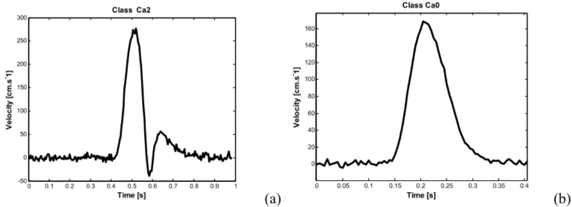
Figure 4 shows a pair of such noisy profiles (with SNR = 20 dB), as constructed from two of the profiles presented in Figure 3.
A first evaluation of performance based on the percentages of successful extractions, using corrupted profiles with SNR of 20 dB has been run. In this experiment, a solution was accepted if the signal to noise ratio (SNR) of the reconstructed profile was greater than an arbitrary threshold of 10 dB. As one can see in Table 3, XZERO performed better than INFLEX and INITRI under these noisy conditions, and the combined system IIX converged in more than 98% of the cases.
-0 0.1 0.2 0.3 0.4 0.5 0.6 0.7 0.8 0.9 1 -50 0 50 100 150 200 250 300 Time [s] Ve lo ci ty [c m .s -1] Class Ca2 (a) 0 0.05 0.1 0.15 0.2 0.25 0.3 0.35 0.4 0 20 40 60 80 100 120 140 160 Time [s] Ve lo ci ty [c m .s -1] Class Ca0 (b)
Fig 4. Two noisy Delta-Lognormal profiles that correspond to two of the ideal profiles depicted in Figure 3 (classes Ca2 and Ca0, respectively), upon which a 20dB noise has been superimposed.
Since we knew the original parameter values of each noisy curve in this simulation, we could evaluate the performance of the extractor according to its capability to recover, un-der various SNR, the real parameter values within specific confidence intervals.
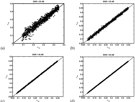
For example, Figure 5 depicts the extracted values of the parameter σ1 vs. the original ones, for SNR equal to 20, 30, 40 and 50 dB respectively. Each plot represents the best extraction result as obtained by the IIX system. For ideal curves, all dots in a plot would be located on the 45o oblique line and, in noisy conditions, the extraction errors result in a
dispersion of the values around this oblique line. As can be observed from these plots, there is a relationship between the dispersion error and the SNR. Indeed, Figure 6a de-picts the extraction error of the parameter σ1 for a SNR equal to 20 dB; these fluctuations look like a random signal. Its histogram (Figure 6b) shows that the error roughly follows a Gaussian process. According to a Kolmogorov-Smirnov test, this histogram can be con-sidered as a normal distribution (h=0, p=0.03), and we can thus evaluate, for each para-meter, the dispersion of the corresponding extraction error through its confidence inter-val. This result suggests that a part of the synthetic Gaussian noise added to the ideal ve-locity profile is transformed into an extraction error that keeps the same distribution. In
-other words, the IIX extractor can be considered as a system that does not generate any additional distortion or noise to the Delta-Lognormal parameters but that translates the noise existing in the original data into extraction errors. In these conditions, confidence intervals can be estimated for the optimal extracted values of the seven parameters.
TABLE 3RESULTS OF THE TESTS UNDER NOISY CONDITIONS IN THE CASE OF SNR=20dB
(CONVERGENCE CRITERION:SNR ≥10 dB) NOISY DATA Algorithms % of convergence ( from 7000 curves) MSEmean [cm2/s2] MSEstd [cm2/s2] SNRmean [dB] SNRstd [dB] INFLEX 63.24 32.90 62.44 21.76 2.13 INITRI 82.90 31.98 60.91 21.62 2.28 XZERO 95.69 30.28 59.32 21.32 2.05 IIX 98.81 28.62 60.20 21.63 2.26 23
-(a) 0 100 200 300 400 500 600 700 800 900 1000 -0.12 -0.1 -0.08 -0.06 -0.04 -0.02 0 0.02 0.04 0.06 0.08 Trial number Δσ 1 SNR = 20 dB (b) -0.15 -0.1 -0.05 0 0.05 0.1 0 2 4 6 8 10 12 14 16 18 Δσ 1 de ns ity SNR = 20 dB
Fig 6. a) Typical result of the extraction error profile of the parameter σ1as obtained for SNR =20 dB and for
the Ca0 class b) Its corresponding histogram assimilated to a Gaussian density, the continuous curve
represents a Gaussian density as calculated by a Kolmogorov-Smirnov test with h=0 and p=0.03.
(a) 0 0.1 0.2 0.3 0.4 0.5 0 0.1 0.2 0.3 0.4 0.5 σ 1o σ1e SNR = 20 dB (b) 0.05 0.1 0.15 0.2 0.25 0.3 0.35 0.4 0.45 0.05 0.1 0.15 0.2 0.25 0.3 0.35 0.4 0.45 0.5 σ 1o σ1e SNR = 30 dB (c) 0.05 0.1 0.15 0.2 0.25 0.3 0.35 0.4 0.45 0.05 0.1 0.15 0.2 0.25 0.3 0.35 0.4 0.45 0.5 σ 1o σ1e SNR = 40 dB (d) 0.05 0.1 0.15 0.2 0.25 0.3 0.35 0.4 0.45 0.05 0.1 0.15 0.2 0.25 0.3 0.35 0.4 0.45 0.5 σ1o σ1e SNR = 50 dB
Fig 5. A typical result of the extracted error dispersion according to SNR values. Representation of the extracted values
versus the original ones for the parameter σ1,at different noise levels.
6.1. Evaluation of the extraction accuracy
The second performance evaluation relied on the circumscription and the quantification of the extractor accuracy by constructing these confidence intervals (CI) for each parame-ter. This has been computed using the optimal parameter values, the MSE and the SNR.
-To do so, the extracted value of a parameter was considered as the center of a confidence interval with extremities calculated from the standard deviation of the correspond-ing extraction error. For example, the CI of the parameter
STD
1
σ was computed by:
1 1 * 1, 1 *
CIσ =⎡⎣σ −k STDσ σ +k STDσ1⎤⎦ (36)
where σ1 is the extracted value, STDσ1the standard deviation of the extraction error
and k the dispersion range (k=1, 2 or 3). Let us recall that for k=2, the original value is inside the CI with a confidence level of 95%.
Since the dispersion decreases when the SNR increases (see Figure 5), one can construct empirical relationships between these quantities and build the confidence inter-vals CI from the SNR values.
STD
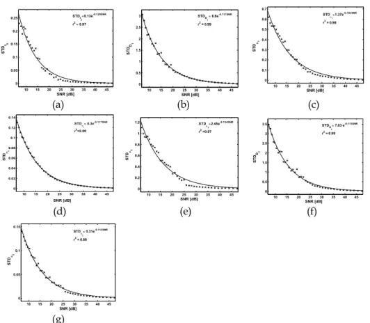
These empirical relationships were calculated as follows: for each Delta-Lognormal pa-rameter, a dispersion parameter of the extraction error was calculated (assuming that the mean value of the error was nearly zero) by considering the 7000 curves of the seven classes, for a given SNR value. The versus SNR curve was then plotted as , for examples, in Figures 7.An exponential relationship emerges from these plots, which can be expressed as:
p STD p STD SNR p STD =αe−β (37) where is the standard deviation of the extraction error for a given parameter p, and
p
STD
α and β are the regression coefficients, as summarized in Table 4 for the seven parameters. According to the definition of the SNR (SNR=10log10
[
P Ps n]
where Psis the-power of the signal and is the power of the Gaussian noise), equation (37) can be rewritten as follows: 2 n P STD= n p s n STD P α = STD (38)
TABLE 4:EXPONENTIAL REGRESSION RESULTS WITH
THE CORRESPONDING CORRELATION COEFFICIENTSr2.
Parameters α β r2 0 t 0.13 0.129 0.97 1 D 6.8 0.117 0.99 1 μ 1.37 0.103 0.98 1 σ 0.3 0.117 0.99 2 D 7.63 0.113 0.99 2 μ 2.45 0.104 0.97 2 σ 0.31 0.113 0.99
Equation (38) clearly reflects the fact that the power of the extraction error (its standard deviation) corresponds to a proportion of the noise added to the velocity profiles. As pre-viously anticipated, this also suggests that the IIX extractor does not add any supplemen-tary noise but “transforms” the existing fluctuations into extraction errors with different proportions.
-10 15 20 25 30 35 40 45 0 0.05 0.1 0.15 0.2 0.25 SNR [dB] ST Dt0 STDt 0 ≈0.13e-0.129SNR r2≈ 0.97 10 15 20 25 30 35 40 45 0 0.5 1 1.5 2 2.5 3 SNR [dB] ST DD1 STDD1 ≈ 6.8e-0.117SNR r2 = 0.99 10 15 20 25 30 35 40 45 0 0.1 0.2 0.3 0.4 0.5 0.6 0.7 SNR [dB] ST Dμ1 STDμ 1 ≈1.37e-0.103SNR r2 = 0.98 (a) (b) (c) 10 15 20 25 30 35 40 45 0 0.02 0.04 0.06 0.08 0.1 0.12 0.14 SNR [dB] ST Dσ 1 STDσ1 ≈ 0.3e-0.117SNR r2=0.99 10 15 20 25 30 35 40 45 0 0.2 0.4 0.6 0.8 1 1.2 SNR [dB] ST Dμ 2 STDμ 2 ≈2.45e-0.104SNR r2 =0.97 10 15 20 25 30 35 40 45 0 0.5 1 1.5 2 2.5 3 3.5 SNR [dB] ST DD2 STDD 2 ≈ 7.63 e-0.113SNR r2 = 0.99 (d) (e) (f) 10 15 20 25 30 35 40 45 0 0.05 0.1 0.15 SNR [dB] ST Dσ2 STDσ2 ≈ 0.31e-0.113SNR r2 = 0.99 (g)
Fig 7. Typical results depicting exponential regressions between the standard deviation of the extraction errors and the SNR of the noisy Delta-Lognormal profiles
This characterization process permits the quantification of the extractor accuracy and the determination of confidence intervals for each extracted parameter value.
7.
T
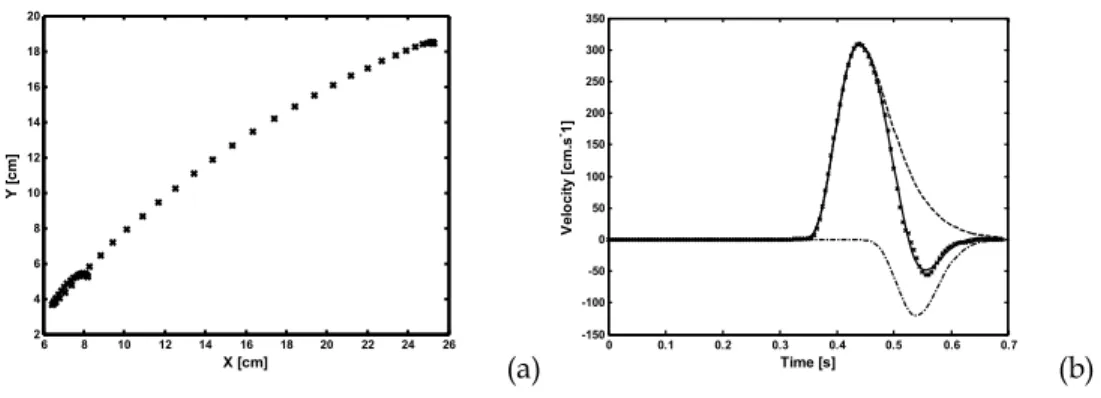
ESTING WITH REAL DATATo evaluate the performance of the IIX extraction system in real applications, we have conducted a third experiment using real handwritten strokes sampled at 200 Hz with a Wacom Intuos II digitizer. Figure 8a depicts a typical x-y trajectory of a stroke produced by a human subject. The corresponding velocity profile, as illustrated in Figure 8b, was computed using numerical filters (a Chebychev II low-pass filter with order n= 10, cutoff frequency Fc= 16 Hz, sampling frequency Fs = 200 Hz, and Attenuation Att= -81 dB, and a FIR derivative filter with n = 10, Fc = 50 Hz and Fs = 200 Hz) applied to the two
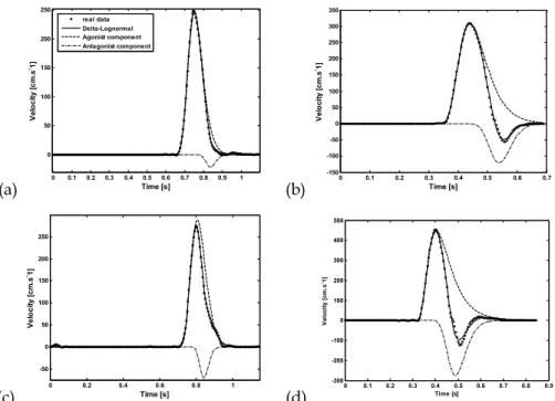
-tion components x(t) and y(t) for each stroke. Representative results of the analysis-by-synthesis process are presented in Figures 9a-d. For each trial, the velocity profile, as re-constructed from the seven extracted parameters, is very close to the original profile with SNR greater than 20 dB. Details of the corresponding parameters with their confidence intervals are summarized in Table 5.
As one can deduct from this Table, the agonist parameters were extracted with more accuracy (extraction uncertainty less than 9 %) than the antagonist ones. This was proba-bly caused by both the architecture of the extractor and the fact that the antagonist para-meter values were small. Indeed, since the antagonist component is isolated after sub-tracting the estimated agonist component, this creates more distortions in the antagonist profile and leads to a poorer estimation of its parameters.
6 8 10 12 14 16 18 20 22 24 26 2 4 6 8 10 12 14 16 18 20 X [cm] Y [c m ] (a) 0 0.1 0.2 0.3 0.4 0.5 0.6 0.7 -150 -100 -50 0 50 100 150 200 250 300 350 Time [s] Ve lo ci ty [c m .s -1] (b)
Fig 8. Typical example of real data. a) stroke trajectory; b) velocity profile (cross: original profile; solid line: reconstructed profile, dashed lines: agonist and antagonist components respectively).
Moreover, since the magnitude of is generally smaller than and becomes often comparable to the magnitude of the noise, it is difficult to get an acceptable precision in some cases. For example, in the velocity profiles depicted in Figure 9-a, the uncertainty grows up to 32% when is small even if the SNR is about 31 dB. However, as depicted in Figures 9-b and 9-d, when the antagonist component is more significant, the corres-ponding uncertainty of its parameters decreases, to less than 20% in these specific results.
2
D D1
2
D
29 -(a) 0 0.1 0.2 0.3 0.4 0.5 0.6 0.7 0.8 0.9 1 0 50 100 150 200 250 Time [s] Ve lo ci ty [c m. s -1] real data Delta-Lognormal Agonist component Antagonist component (b) 0 0.1 0.2 0.3 0.4 0.5 0.6 0.7 -150 -100 -50 0 50 100 150 200 250 300 350 Time [s] Ve lo ci ty [c m .s -1] (c) 0 0.2 0.4 0.6 0.8 1 -50 0 50 100 150 200 250 Time [s] Ve lo ci ty [c m.s -1] (d) 0 0.1 0.2 0.3 0.4 0.5 0.6 0.7 0.8 0.9 -300 -200 -100 0 100 200 300 400 500 Time [s] Ve lo ci ty [c m .s -1]
Figure 9: typical extraction results from different velocity patterns. The corresponding parameter values are summa-rized in Table 5.
TABLE 5.SUMMARY OF EXTRACTED PARAMETER VALUES WITH CONFIDENCE INTERVALS EXPRESSED IN TERMS OF PERCENTAGES. Parame-ter μ2 σ2 MSE SNR (dB) 0 t (s) 1 D μ1 σ1 D2 (cm2.s-2) (cm) (cm) Trial # a 0.567 +/- 1.3% 24.733 +/- 1.56% -1.651 +/-4.72% 0.212 +/-8.04% 1.32 +/- 32.86% -1.3 +/-10.71% 0.091 +/-19.37% 4.86 31.79 b 0.302 +/- 3.8% 38.214 +/- 1.31% -1.867 +/-5.42% 0.338 +/-6.56% 10.876 +/- 5.18% -1.418 +/-18.76% 0.15 +/- 15.26% 20.66 29.45 c 0.603 +/- 0.94% 29.762 +/- 0.99% -1.556 +/-3.85% 0.199 +/-6.58% 4.204 +/-7.93% -1.421 +/-7.53% 0.099 +/- 13.62% 4.15 34.14 d 0.3 +/- 5.79% 61.22 +/- 1.48% -2.046 +/-8.95% 0.471 +/-8.52% 27.703 +/- 3.68% -1.626 +/-20.15% 0.209 +/- 19.84% 92.58 24.15 30
-8.
C
ONCLUSIONIn this paper, we have focused on the analysis-by-synthesis of individual strokes, i.e. the study of motor control primitives. Using the Kinematic Theory, which completely describes the velocity profile of rapid movement with seven Delta-Lognormal parame-ters, we have developed an efficient parameter extractor system that relies on a new algo-rithm (XZERO). This algoalgo-rithm exploits the properties of the first and the second time-derivatives of a lognormal function. We have highlighted the performance improvements that are observed by this new estimation method in comparison with two existing ones (INFLEX and INITRI). For ideal curves, XZERO finds the true values of Delta-Lognormal parameters in 97% of the cases, for a database of 7000 curves representing a huge variety of patterns. Moreover, the complementarities that exist between the three algorithms (INFLEX, INITRI and XZERO) have leaded us to combine them in a new ar-chitecture, the IIX system, to improve the global performances.
We have also circumscribed and quantified the confidence intervals of the extracted values, exploiting the empirical exponential regressions that link the standard deviation (STD) of the extraction error with the SNR. Thus, the optimal values of the parameters used to reconstruct the velocity profiles of rapid movements by a Delta-Lognormal equa-tion are, for the first time, accompanied with precision estimates, which quantify their relative validity.
One useful application of this new information is for the calibration of Delta-Lognormal measurement systems. Although more works will be necessary to apply this technology to the study of complex movements like handwriting, the present tool already offers the possibility of analyzing the behavior of neuromuscular and motor control
-tems under various experimental and psychophysical conditions, through the variations in the parameter values.
With this robust extractor, the Kinematic Theory will become more attractive for the study of movement primitives. Current experiments are going on in our laboratory, where, for example, our algorithms are applied to analyze the intrinsic properties of strokes produced by different group of participants ( young and aged subjects, male and female, etc) [6,44], and to provide a better understanding of these primitives and their use as building blocks for the automatic processing of handwriting in various fields of computer science [2],[3]. In its present form, the IIX system is not limited to human movement applications. It could be employed to analyze any lognormal processes. Its ge-neralization and adaptation to the study of more complex patterns is under way.
ACKNOWLEDGEMENTS
This research work was supported by NSERC grant RGPIN-915 to Réjean Plamondon.
REFERENCES
[1] M. Djioua and R. Plamondon, “Analysis and Synthesis of Handwriting Variability using the Sigma-Lognormal Model,” Proceeding of the 13th Conference of the International Gra-phonomics Society (IGS2007), vol 13, pp. 19-22, 2007.
[2] R. Plamondon and M. Djioua, "A multi-level representation paradigm for handwriting stroke generation,” Human Movement Science, vol. 25, pp. 586-607, 2006.
[3] R. Plamondon, and M. Djioua, “Handwriting Stroke Trajectory Variability in the con-text of the Kinematic Theory,” Proceeding of the 12th Conference of the International Graphonomics Society (IGS2005),, vol 12, pp. 250–254, 2005.
-[4] R. Plamondon, and S. Srihari, “On-line and off-line handwriting recognition: A compre-hensive survey,” 20th Anniversary Special Issue. IEEE Trans. On Pattern Analysis and Machine Intelligence, vol. 22, pp. 63–84, 2000.
[5] R. Plamondon, D. Lopresti, L.R.B. Schomaker, and S. Srihari, “On-line handwriting recognition,” In J. G. Webster (Ed.). Wiley Encyclopedia of Electrical and Electronics Engineering , vol. 15, pp. 123-146, 1999, NY: John Wiley & Sons, ISBN0-471-13946-7. [6] A. Woch, "Étude des primitives bidirectionnelles du mouvement dans le cadre de la théorie cinématique: confirmation expérimentale du modèle delta-lognormal," PhD dis-sertation, Dept. of Electrical, École Polytechnique de Montréal, 2006.
[7] A. Woch and R. Plamondon, "The problem of Movement Primitives in the Context of the Kinematic Theory," Proceeding of the 11th Conference of the International Grapho-nomics Society (IGS2003), Scottsdale, Arizona, USA, vol. 11, pp. 67-71, 2003.
[8] A. Woch and R. Plamondon, "Using the Framework of the Kinematic Theory for the Definition of a Movement Primitive," Motor Control, vol. 8, pp. 547-557, 2004.
[9] S. F. Giszter, F. A. Mussa-Ivaldi, and E. Bizzi, "Convergent Force Field Organized in the Frog’s Spinal Cord," Journal of Neuroscience, vol. 13, pp. 467-491, 1993.
[10] F. A. Mussa-Ivaldi, S. F. Giszter, and E. Bizzi, "Linear combinations of primitives in vertebrate motor control," Proceedings of the National Academy of Sciences, USA, vol. 91(16), pp. 7534-7538,1994.
[11] R. W. Paine and J. Tani, "Motor primitive and sequence self-organization in a hierar-chical recurrent neural network," Neural Network, vol. 17, pp. 1291-1309, 2004.
[12] K. A. Thoroughman and R. Shadmehr, "Learning of action through adaptive combi-nation of motor primitives," Nature, vol. 407, pp. 742-747, 2000.
-[13] O. Hilton, “Scientific Examination of Questioned Documents,” In CRC series in fo-rensic and police science, 1993, CRC Press, Boca Raton, London, revised edition.
[14] M.L. Simner and P.L. Girouard (Eds.), “Advance in forensic document examination [Special issue],” Journal of Forensic Document Examination, vol. 13, pp. 1–14, 2000. [15] M.L. Simner, C.G. Leedham, and A. J. W. M. Thomassen, (Eds.), “Handwriting and
drawing research: Basic and applied issues,” Amsterdam: IOS Press, 1996.
[16] J. Wann, A.M. Wing, and N. Søvik, “Development of graphic skills: Research, pers-pectives and education implications. London: Academic Press, 1991.
[17] A. Schröter, R. Mergl, K. Bürger, H. Hampel, H.-J Möller and U. Hegerl, ”Kinematic analysis of handwriting movements in patients with Alzheimer’s disease, mild cognitive impairment, depression and healthy subjects,” Dementia and Geriatric Cognitive Disord-ers, vol. 15, pp. 132–142, 2003.
[18] H. L. T. Teuling and G.E. Stelmach,”Control of stroke size, peak acceleration and stroke duration in Parkinsonian handwriting,” Human Movement Science, vol. 10, pp. 315–333, 1991.
[19] B. Rohrer, S. Fasoli, H.I. Krebs, R. Hughes, B. Volpe, and W.R. Frontera, “Move-ment smoothness changes during stroke recovery”, Journal of Neuroscience, vol. 22, pp. 8297–8304, 2002.
[20] V. Potkonjak, “Robotic handwriting”, International Journal of Humanoid Robotics, vol. 2, pp.105–124, 2005.
[21] F. Lacquaniti, C. Terzuolo, and P. Viviani, "The law relating the kinematic and figur-al aspects of drawing movements," Acta Psychologica, vol. 54, pp. 115-130, 1983.
-[22] P. Morasso, "Spatial control of arm movements," Experimental Brain Research, vol. 42, pp. 223-227, 1981.
[23] J. Soechting and F. Lacquaniti, "Invariant characteristics of a pointing movement in man," Journal of Neuroscience, vol. 1, pp. 710-720, 1981.
[24] P. Viviani and C. Terzuelo, "Space-time invariance in learned motor skills,” In: Stelmach GE, Requin J (eds) Tutorials in motor behavior. North-Holland, Amster-dam, pp 525–533, 1980.
[25] R. Plamondon, "A kinematic theory of rapid human movements Part I. Movement representation and generation," Biological Cybernetics, vol. 72, pp. 295-307, 1995. [26] R. Plamondon and W. Guerfali, "The generation of handwriting with delta-lognormal
synergies,” Biological Cybernetics, vol. 78, pp. 119-132, 1998.
[27] W. Guerfali, "Modèle Delta-lognormal vectoriel pour l’analyse du mouvement et la génération de l’écriture manuscrite," Ph.D. dissertation, Dept. of Electrical, École Poly-technique de Montréal, 1996.
[28] F. Leclerc, " Modèle de génération de mouvements rapides en représentation de si-gnatures manuscrites," Ph.D. dissertation, Dept. of Electrical, École Polytechnique de Montréal, 1996.
[29] A. C. Cohen and B. J. Whitten, "Estimation in the Three-Parameter Lognormal Dis-tribution," Journal of the American Statistical Association, vol. 75(370), pp. 399-404, 1980.
[30] E. L. Crow and K. Shimizu (Eds.), “Lognormal distributions: theory and applica-tions,” vol. 88, Dekker, 1988.
-[31] W. Guerfali and R. Plamondon, "Signal processing for the Parameter Extraction of the Delta Lognormal Model," Research in Computer and Robot Vision, pp. 217-232, 1995.
[32] R. Plamondon, X. Li, M.Djioua, “Extraction of delta-lognormal parameters from handwriting strokes,” Journal of Frontiers of Computer Science in China, vol 1(1), pp:106-113, 2007.
[33] M. Djioua, R. Plamondon, A. Della Cioppa, A., Marcelli, “Delta-lognormal parame-ter estimation by non-linear regression and evolutionary algorithm: A comparative study,” Proceeding of the 12th Conference of the International Graphonomics Society (IGS2005), vol. 12, pp. 44-48, 2005.
[34] M. Djioua, R. Plamondon, A. Della Cioppa, A., Marcelli, “Deterministic and evolu-tionary extraction of Delta-Lognormal parameters: performance comparison,” Interna-tional Journal of Pattern Recognition and Artificial Intelligence, vol. 21(1), pp. 21-41, 2007.
[35] T. Varga, D. Kilchhofer, H. Bunke, “Template-based Synthetic Handwriting Genera-tion for the Training of RecogniGenera-tion Systems,” Proceeding of the 12th Conference of the International Graphonomics Society (IGS2005), vol. 12 , pp. 206-211, 2005.
[36] R. Plamondon, A. M. Alimi, P. Yergeau, and F. Leclerc, "Modelling velocity profiles of rapid movements: a comparative study," Biological cybernetics, vol. 69(2), pp. 119-128, 1993.
[37] A. Alimi, "Contribution au développement d’une théorie de génération de mouve-ments simples et rapides:application au manuscrit," Ph.D. dissertation, Dept. of Electri-cal, École Polytechnique de Montréal, 1995.
37
-[38] A. Alimi and R. Plamondon, "A comparative study of speed/accuracy tradeoff formu-lations: The case of spatially constrained movements where both distance and spatial pre-cision are specified," in M. L. Simner, G.Thomassen, A.J.T.W.M., Eds. Handwriting and drawing research: basic and applied issues. IOS Press, Amsterdam, pp. 127-142, 1996. [39] C. Feng, A. Woch, and R. Plamondon, "A Comparative Study of Two Velocity
Pro-file Models for Rapid Stroke Analysis," Proceeding of the 16th International Conference on Pattern Recognition, Quebec, Canada, vol. 4, pp. 52-55, 2002.
[40] M. Djioua, "Contributions à la généralisation, à la compréhension et à l’utilisation de la théorie cinématique dans l’analyse et la synthèse du mouvement humain," Ph.D. dis-sertation, Dept. of Electrical, École Polytechnique de Montréal, 2007.
[41] R. Plamondon, "A kinematic theory of rapid human movements. Part II. Movement time and control," Biological Cybernetics, vol. 72, pp. 309-320, 1995.
[42] R. Plamondon, C. Feng, and A. Woch, "A kinematic theory of rapid human move-ment. partIV: a formal mathematical proof and new insights," Biological Cybernetics, vol. 89, pp. 126–138, 2003.
[43] D. W. Marquardt "An algorithm for least-squares estimation of non-linear parame-ters," Journal of the Society of Industrial and Applied Mathematics, vol. 11, pp. 431-441, 1963.
[44] A. Woch and R. Plamondon, “Analysis of movement primitives with the DL model: in-sights on the age effect,” Proceeding of the 13th Conference of International Graphonom-ics Society (IGS2007), vol. 13, pp. 56-59, 2007.