Factor analysis of dynamic PET images

(1)

En vue de l'obtention du

DOCTORAT DE L'UNIVERSITÉ DE TOULOUSE

Délivré par :

Institut National Polytechnique de Toulouse (Toulouse INP)

Discipline ou spécialité :

Signal, Image, Acoustique et Optimisation

Présentée et soutenue par :

Mme YANNA CRUZ CAVALCANTI

le mercredi 31 octobre 2018

Titre :

Unité de recherche :

Ecole doctorale :

Factor analysis of dynamic PET images

Mathématiques, Informatique, Télécommunications de Toulouse (MITT)

Institut de Recherche en Informatique de Toulouse (I.R.I.T.)

Directeur(s) de Thèse :

M. NICOLAS DOBIGEON M. CLOVIS TAUBER

Rapporteurs :

Mme IRÈNE BUVAT, CNRS PARIS

M. SAID MOUSSAOUI, ECOLE CENTRALE NANTES

Membre(s) du jury :

M. CHRISTIAN JUTTEN, UNIVERSITE JOSEPH FOURIER, Président M. ANTOINE SOULOUMIAC, CEA SACLAY, Membre

M. CLOVIS TAUBER, UNIVERSITE DE TOURS, Membre Mme CAROLINE PETITJEAN, UNIVERSITE DE ROUEN, Membre

M. NICOLAS DOBIGEON, INP TOULOUSE, Membre M. SIMON STUTE, CEA GRENOBLE, Invité M. THOMAS OBERLIN, INP TOULOUSE, Membre

(2)

(3)

A Deus, por sua generosidade nas bençãos que me concede. À minha mãe, por me dar a vida e me permitir vivê-la em plenitude. Ao meu marido Vinicius, que esteve ao meu lado em cada passo dessa longa jornada pelo conhecimento. “Tudo posso naquele que me fortalece.” Filipenses 4:13

(4)

(5)

Acknowledgments

The journey in the search for knowledge is challenging and everlasting. It often requires eﬀort, commitment, persistence and a lot of resilience. My journey has only just begun, but a big step has deﬁnitely been taken. The obstacles that have come into my way until this day could never be overcome without the support and encouragement of the people there are to be referred to.

First and foremost, I would like to express my sincere gratitude to my supervisors Dr Nicolas Dobigeon, Dr Clovis Tauber and Dr Thomas Oberlin for giving me the opportunity to achieve this Ph.D. thesis. I am also thankful for their guidance, patience, constructive criticism and advice, which have enabled me to complete this project successfully. Additionally, I would like to acknowledge the bureaucratic support from Dr Dobigeon in my arrival in France and many other moments throughout this Ph.D. Dr Dobigeon has also been my professor during graduation and has inspired me with his knowledge to pursue research. Along with Dr Clovis Tauber, he gave me my ﬁrst professional opportunity in a short internship at IRIT in 2012, for which I am truly grateful to both of them.

For this dissertation, I would like to thank Dr Irène Buvat and Dr Said Moussaoui for taking the time, despite their busy schedules, to study my work and report on my thesis. I would also like to thank Dr Christian Jutten for accepting to chair my jury and the board of examiners, Dr Caroline Petitjean and Dr Antoine Souloumiac, for their time and insightful questions. Additionally, I thank Dr Simon Stute for accepting the invitation to attend my thesis defence and providing me with the datasets that I needed for my simulations.

This thesis work would not have been successful without the scientiﬁc collaboration of many people. In particular, I would like to thank Dr Cédric Févotte and Dr Vinicius Ferraris for the stimulating discussions.

I gratefully acknowledge the funding sources that made my Ph.D. work possible. I was funded by the Brazilian Ministry of Education in a 3-year international doctorate program. I hope to have the opportunity of bringing back to Brazil all the knowledge and experience that I have acquired in France since my graduation (also ﬁnanced by the Brazilian government). I believe that science and technology have the power of changing the world. My main goal in everything that I have done so far is to be able to improve people’s lives through knowledge. Thus, I hope with all my heart to have the opportunity to bring science to people, allowing technology to change their lives through my work.

(6)

Mrs Annabelle Sansus and Mrs Isabelle Vasseur that do a remarkable work for all IRIT members. I would also like to thank all the members of the SC group that have contributed immensely to my personal and professional time at IRIT. I thank my past and current fellow labmates: Adrien, Louis, Olivier, Dylan, Mouna, Jessica, Pierre-Antoine, Tatsumi, Etienne and Baha for the enormous support, great conversations and pleasant companionships. I could not also forget all the other past and current members of the SC group: Sébastien, Marie, Herwig, Charly, Benoît, Claire, Yassine, Alberto, Maxime and Dana. I would also like to thank the members of the Inserm laboratory for their hospitality during my short stay at Tours.

Above all, I would like to thank my family for all their love and encouragement. I thank my parents, Lucimar e Yêso, who supported me in all my pursuits. Their constant love and encouragement is the foundation on which everything else is built. I thank my grandmother Paulina for her love and prayers. Finally, I thank my loving, encouraging, and patient husband Vinicius whose faithful support kept me going. To all of you, I dedicate this thesis.

(7)

Abstract

Thanks to its ability to evaluate metabolic functions in tissues from the temporal evolution of a previously injected radiotracer, dynamic positron emission tomography (PET) has become an ubiquitous analysis tool to quantify biological processes. Several quantiﬁcation techniques from the PET imaging literature require a previous estimation of global time-activity curves (TACs) (herein called factors) representing the concentration of tracer in a reference tissue or blood over time. To this end, factor analysis has often appeared as an unsupervised learning solution for the extraction of factors and their respective fractions in each voxel.

Inspired by the hyperspectral unmixing literature, this manuscript addresses two main drawbacks of general factor analysis techniques applied to dynamic PET. The first one is the assumption that the elementary response of each tissue to tracer distribution is spatially homogeneous. Even though this homogeneity assumption has proven its effectiveness in several factor analysis studies, it may not always provide a sufficient description of the underlying data, in particular when abnormalities are present. To tackle this limitation, the models herein proposed introduce an additional degree of freedom to the factors related to specific binding. To this end, a spatially-variant perturbation affects a nominal and common TAC representative of the high-uptake tissue. This variation is spatially indexed and constrained with a dictionary that is either previously learned or explicitly modelled with convolutional nonlinearities affecting non-specific binding tissues. The second drawback is related to the noise distribution in PET images. Even though the positron decay process can be described by a Poisson distribution, the actual noise in reconstructed PET images is not expected to be simply described by Poisson or Gaussian distributions. Therefore, we propose to consider a popular and quite general loss function, called the β-divergence, that is able to generalize conventional loss functions such as the least-square distance, Kullback-Leibler and Itakura-Saito divergences, respectively corresponding to Gaussian, Poisson and Gamma distributions. This loss function is applied to three factor analysis models in order to evaluate its impact on dynamic PET images with different reconstruction characteristics.

Keywords: dynamic PET images, blind source separation, unsupervised learning, non-convex optimization, majorization-minimization algorithms.

(8)

(9)

Résumé

La tomographie par émission de positrons (TEP) est une technique d’imagerie nucléaire non-invasive qui permet de quantifier les fonctions métaboliques des organes à partir de la diffusion d’un radiotraceur injecté dans le corps. Alors que l’imagerie statique est souvent utilisée afin d’obtenir une distribution spatiale de la concentration du traceur, une meilleure évaluation de la cinétique du traceur est obtenue par des acquisitions dynamiques. En ce sens, la TEP dynamique a suscité un intérêt croissant au cours des dernières années, puisqu’elle fournit des informations à la fois spatiales et temporelles sur la structure des prélèvements de traceurs en biologie in

vivo. Les techniques de quantiﬁcation les plus eﬃcaces en TEP dynamique nécessitent souvent une estimation

de courbes temps-activité (CTA) de référence représentant les tissus ou une fonction d’entrée caractérisant le ﬂux sanguin. Dans ce contexte, de nombreuses méthodes ont été développées pour réaliser une extraction non-invasive de la cinétique globale d’un traceur, appelée génériquement analyse factorielle.

L’analyse factorielle est une technique d’apprentissage non-supervisée populaire pour identifier un modèle ayant une significat physique à partir de données multivariées. Elle consiste à décrire chaque voxel de l’image comme une combinaison de signatures élémentaires, appelées facteurs, fournissant non seulement une CTA globale pour chaque tissu, mais aussi un ensemble des coefficients reliant chaque voxel à chaque CTA tissulaire. Parallèlement, le démélange - une instance particulière d’analyse factorielle - est un outil largement utilisé dans la littérature de l’imagerie hyperspectrale. En imagerie TEP dynamique, elle peut être très pertinente pour l’extraction des CTA, puisqu’elle prend directement en compte à la fois la non-négativité des données et la somme-à-une des proportions de facteurs, qui peuvent être estimées à partir de la diffusion du sang dans le plasma et les tissus.

Inspiré par la littérature de démélange hyperspectral, ce manuscrit s’attaque à deux inconvénients majeurs des techniques générales d’analyse factorielle appliquées en TEP dynamique. Le premier est l’hypothèse que la réponse de chaque tissu à la distribution du traceur est spatialement homogène. Même si cette hypothèse d’homogénéité a prouvé son efficacité dans plusieurs études d’analyse factorielle, elle ne fournit pas toujours une description suffisante des données sous-jacentes, en particulier lorsque des anomalies sont présentes. Pour faire face à cette limitation, les modèles proposés ici permettent un degré de liberté supplémentaire aux facteurs liés à la liaison spécifique. Dans ce but, une perturbation spatialement variante est introduite en complément d’une CTA nominale et commune. Cette variation est indexée spatialement et contrainte avec un dictionnaire,

(10)

qui est soit préalablement appris ou explicitement modélisé par des non-linéarités convolutives aﬀectant les tissus de liaisons non-spéciﬁques. Le deuxième inconvénient est lié à la distribution du bruit dans les images PET. Même si le processus de désintégration des positrons peut être décrit par une distribution de Poisson, le bruit résiduel dans les images TEP reconstruites ne peut généralement pas être simplement modélisé par des lois de Poisson ou gaussiennes. Nous proposons donc de considérer une fonction de coût générique, appelée

β-divergence, capable de généraliser les fonctions de coût conventionnelles telles que la distance euclidienne, les

divergences de Kullback-Leibler et Itakura-Saito, correspondant respectivement à des distributions gaussiennes, de Poisson et Gamma. Cette fonction de coût est appliquée à trois modèles d’analyse factorielle aﬁn d’évaluer son impact sur des images TEP dynamiques avec diﬀérentes caractéristiques de reconstruction.

Mots-clés: images TEP dynamiques, séparation aveugle des sources, apprentissage non supervisé, optimi-sation non convexe, algorithmes de majoration-minimioptimi-sation.

(11)

(12)

Abbreviations

ADMM Alternated direction method of multipliers ANC Abundance nonnegativity constraint ASC Abundance sum-to-one constraint AUC Area under the curve

BCCB Block circulant matrix with circulant blocks BCD Block-coordinate descent

BCM Beta compositional model BPT Binary partition trees BSS Blind source separation

CAPES Coordenação de Aperfeiçoamento de Ensino Superior CLS Constrained least squares

CLT Central limit theorem CM Compartmental modelling CT Computed tomography DPE Doutorado Pleno no Exterior ECG Electrocardiograms

EEG Electroencephalograms ELMM Extended linear mixing model EM Expectation maximization EMG Electromyograms

FADS Factor analysis of dynamic structures FBP Filtered-back projection

FCLS Fully constrained least squares

fMRI Functional magnetic resonance imaging FOV Field-of-view

FRTM Full reference tissue compartment model

(13)

GNCM Generalized normal compositional models ICA Independent component analysis

INSERM Institut National de la Santé et de la Recherche Médicale KL Kullback-Leibler

LMM Linear mixing models LOR Line-of-response LRM Local reference model

MLE Maximum likelihood estimators MM Maximization-minimization MNF Minimum noise fraction MRI Magnetic resonance image NCM Normal compositional models NMF Nonnegative matrix factorization NMSE Normalized mean square error nSB Non-speciﬁc binding

OSEM Ordered subset expectation maximization OSP Orthogonal subspace projection

PALM Proximal alternating linearized minimization PCA Principal component analysis

PET Positron emission tomography PLMM Perturbed linear mixing model

PNMM Parametrically nonlinear mixing model PSF Point spread function

PSNR Peak signal-to-noise ratio PVE Partial volume eﬀect Q-Q Quantile-Quantile

rLMM Robust linear mixing model

rNMF Robust nonnegative matrix factorization ROI Regions-of-interest

(14)

SBF Speciﬁc binding factor

SLMM Speciﬁc binding linear mixing model

SUnSAL Sparse unmixing by variable splitting and augmented Lagrangian SUV Standardized uptake value

SVCA Supervised cluster analysis SVD Singular value decomposition SVM Support vector machine TAC Time-activity curve TOF Time-of-ﬂight TSPO Translocator protein VCA Vertex component analysis

List of Figures

1.1 PET acquisition scheme . . . 11

1.2 Illustration of a β+ _{decay [}_JP05_{] . . . .} ₁₂

1.3 Non-collinearity due to conservation of the momentum. [JP05] . . . 13

1.4 Detection of positron annihilation . . . 13

1.5 Illustration of annular arrays of small crystals [JP05]. View of a PET scanner from the annular plane (left) and view along the axis of the scanner (right). . . 15

1.6 Eﬀects of the interaction of radiation with matter [JP05] . . . 16

1.7 Line-of-response (right) and point correspondent to the LOR in a sinogram (left) [Rey07] . . . . 17

1.8 Illustration of a 3D+time dynamic PET image. . . 20

1.9 The transaxial resolution includes a tangential component and a radial component. By moving the radioactive source away from the tomographic axis, the probability that the incident photons interact with the scintillators of several detectors before being absorbed increases. It is therefore more diﬃcult to deﬁne precisely the place of interaction of the 511 keV gamma rays when the distance to the axis increases, this is why the spatial resolution is degraded in this direction [MAI12]. . . 21

1.10 Tissue-fraction effect due to sampling. (B) spill-out of the black structure with the value of 10 over the gray structure with the value of 5, (C) spill-in of the gray structure into the black one, (D) final result from both spill-in and spill-out effects.[SBB07] . . . 22

1.11 Conﬁguration of the classic three-compartment kinetic model used in many imaging studies. . . . 25

1.12 Conﬁguration of the classic three-compartment kinetic model used in many imaging studies. . . . 26

1.13 Conﬁguration of the classic reference three-tissue kinetic model used in many imaging studies. . . 27

2.1 A measured PET voxel is composed by the contributions of each ROI tissue TAC in the corre-sponding studied region. . . 36

2.2 Illustration of a mixing system . . . 38

2.3 Illustration of the factor analysis scheme . . . 44

2.4 An observed hyperspectral voxel is composed by the contributions of each material in the ﬁnal spectral response. . . 45

2.5 Illustration of the simplex for a mixing matrix of 3 factors (a similar representation was introduced in [Bar80]). The ﬁlled circles represent the vertices of the simplex, corresponding to the factors and empty circles are the TACs. . . 46

2.6 Photons interacting with several materials produces nonlinearities. . . 50

2.7 Illustration of a simplex with : (a)endmember without variability,(b)endmember bundles and (c)endmembers as a multivariate probability distribution [HDT15]. . . 53

3.1 Samples of TACs inside the high-uptake region (thalamus for healthy subjects and thalamus plus stroke for unhealthy subjects) of 10 real images of diﬀerent patients, as delimitated by a specialist. 62 3.2 Simplex with one varying factor. . . 63

(18)

List of Figures

3.3 Graphical representation of SLMM. . . 64

3.4 Estimation scheme . . . 67

3.5 Diagram of voxel neighbourhood structure for three dimensions, where the blue voxel is the one considered and the red ones are its direct neighbours. . . 67

3.6 15th_{time-frame of the dynamic PET phantom: from left to right, transversal, sagittal and coronal} views. . . 74

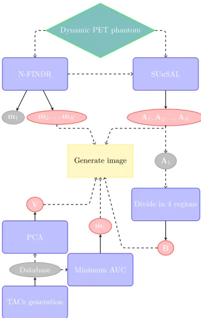
3.7 Synthetic image generation scheme. The red ellipses constitute the ground truth data used for quantitative assessment. . . 74

3.8 Ground truth of factors (right) and corresponding proportions(left), extracted from SUnSAL/N-ﬁndr . . . 76

3.9 Left: variability basis element v1 identiﬁed by PCA. Right: generated SBFs (blue) and the nominal SBF signature (red). . . 77

3.10 Variability matrix B randomly generated. . . 77

3.11 15th_{time-frame of 3D-generated image with PSF and a 15dB noise: from left to right, transversal,} sagittal and coronal planes. . . 77

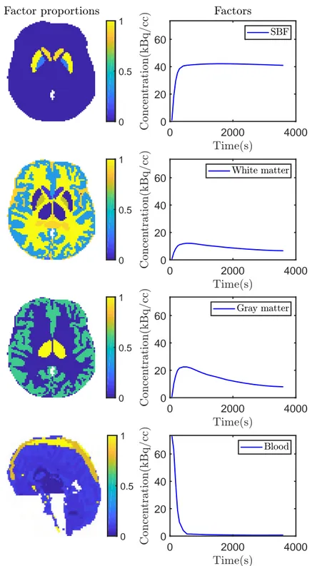
3.12 Factor proportion maps of the 15th _{time-frame obtained for SNR=15dB corresponding to the} speciﬁc gray matter, white matter, gray matter and blood, from left to right. The ﬁrst 3 columns show a transaxial view while the last one shows a sagittal view. All images are in the same scale [0, 1]. . . . 80

3.13 TACs obtained for SNR = 15dB. For the proposed SLMM algorithm, the represented SBF TAC corresponds to the empirical mean of the estimated spatially varying SBFs m1,1, . . . , m1,N. . . . 81

3.14 Ground-truth (left) and estimated (right) SBF variability. . . 81

3.15 Factor proportion maps of the 15t_{h time-frame obtained for SNR=15dB corresponding to the} speciﬁc gray matter, white matter, gray matter and blood, from left to right. The ﬁrst 3 columns show a transaxial view while the last one shows a sagittal view. . . 84

3.16 TACs obtained for SNR=15dB. For the proposed SLMM algorithm, the represented SBF corre-sponds to the empirical mean of the estimated spatially varying SBFs m1,1, . . . , m1,N. . . 85

3.17 Ground-truth (left) and estimated (right) SBF variability. . . 85

3.18 Variability basis elements of ﬁrst subject (left) and second subject (right) . . . 86

3.19 Factor proportion maps of the first stroke subject. The first 3 columns show a transaxial view while the last one shows a sagittal view. From left to right: the specific gray matter, white matter, non-specific gray matter and blood. . . 88

3.20 TACs obtained by estimation from the ﬁrst subject image. . . 89

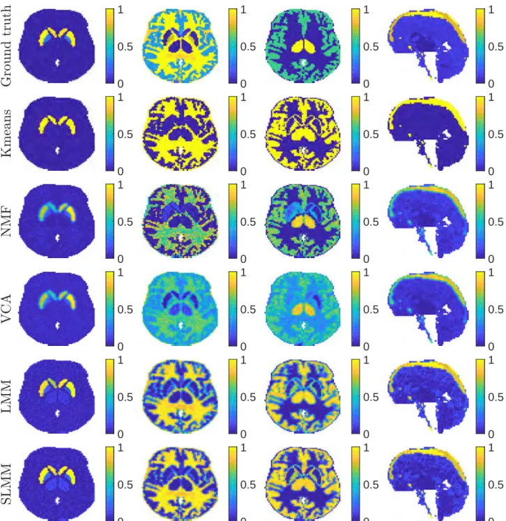
3.21 From top to bottom: MRI ground-truth of the stroke area for the ﬁrst stroke subject, SBF coeﬃcient maps estimated by K-means, NMF, VCA, LMM, SLMM and SBF variability estimated by SLMM. . . 90

3.22 Factor proportion maps of the second stroke subject. The first 3 columns show a transaxial view while the last one shows a sagittal view. From left to right: the specific gray matter, white matter, non-specific gray matter and blood. . . 91

3.23 TACs obtained by estimation from the second stroke subject image. . . 92

3.24 From top to bottom: MRI ground-truth of the stroke area for the second stroke subject, SBF coeﬃcient maps estimated by K-means, NMF, VCA, LMM, SLMM and SBF variability estimated by SLMM. . . 93

4.1 Empirical covariance, mean and variance of a randomly chosen region. . . 101

4.2 Empirical SNR for each frame of time (in dB) . . . 102

4.3 Histogram study in 4 diﬀerent regions of the image and 4 diﬀerent time frames . . . 104

4.4 β-divergence dβ(y = 1|x) as a function of x. . . . 106

4.5 15th_{time-frame of 6it image: from left to right, transversal, sagittal and coronal planes. . . .} ₁₁₆

4.6 15th_{time-frame of 50it image: from left to right, transversal, sagittal and coronal planes. . . . .} ₁₁₆

4.7 PSNR mean and standard deviation obtained on the 6it (left) and 50it (right) images after factorization with β-NMF with fixed (top) and estimated (bottom) factor TACs over 64 samples. 118 4.8 PSNR mean and standard deviation obtained on the 6it (left) and 50it (right) images after factorization with β-LMM with fixed (top) and estimated (bottom) factor TACs over 64 samples.120 4.9 From left do right: factor proportions from specific gray matter, non-specific gray matter, white matter and blood for one 6it sample, estimated with fixed M. . . . 122

(19)

4.10 Variability matrices estimated with ﬁxed M on a 6it sample. . . . 122

4.11 From left do right: factor proportions from specific gray matter, non-specific gray matter, white matter and blood for one 50it sample, estimated with fixed M. . . . 123

4.12 Variability matrices estimated with ﬁxed M on a 50it sample. . . . 123

4.13 From left do right: factor proportions from speciﬁc gray matter, non-speciﬁc gray matter, white matter and blood for one 6it sample. . . 124

4.14 β-SLMM TACs for β = 0, 1, 2 corresponding to the speciﬁc binding factor, gray matter, white matter and blood for one 6it sample. . . 125

4.15 Variability matrices estimated on a 6it sample. . . 125

4.16 From left do right: factor proportions from speciﬁc gray matter, non-speciﬁc gray matter, white matter and blood for one 50it sample. . . 126

4.17 β-SLMM TACs for β = 0, 1, 2 corresponding to the speciﬁc binding factor, gray matter, white matter and blood for one 50it sample. . . 127

4.18 Variability matrices estimated on a 50it sample. . . 127

4.19 From left do right: factor proportions from non-speciﬁc gray matter, white matter and blood obtained with β-SLMM for β = 0, 1, 2. . . . 130

4.20 From top to bottom: MRI ground truth of the stroke zone, factor proportions from speciﬁc gray matter and variability matrices obtained with β-SLMM for β = 0, 1, 2. . . . 132

4.21 TACs corresponding to the speciﬁc binding factor, gray matter, white matter and blood. . . 133

5.1 Synthetic image generation scheme. The red ellipses constitute the ground truth data used for quantitative assessment. . . 144

5.2 Ground truth of factors (right) and corresponding proportions(left), extracted by SUnSAL/N-ﬁndr145

5.3 Binding potential maps w.r.t. the free fraction of radioligand per tissue. . . 146

5.4 Factors (blue) and TACs generated from the 2-tissue reference model. . . 147

5.5 15th_{time frame of 3D-generated image with PSF and a 15dB noise: from left to right, transversal,}

sagittal and coronal planes. . . 147

5.6 Factor proportion maps obtained from the synthetic image corresponding to the gray matter, white matter and blood, from left to right. The ﬁrst 2 columns show a transaxial view while the last one shows a sagittal view. All images are in the same scale [0, 1]. . . . 150

5.7 Factor TACs estimated from the synthetic image . . . 151

5.8 From top to bottom: ground-truth, initial and PNMM estimations of BP.fT. The ﬁrst column

corresponds to the gray matter and the second to the white matter. Note that for DEPICT

BP.fT was estimated for the whole image using the respective tissue TAC as reference. . . 151

5.9 From left to right: SLMM factor proportion related to the SBF, SLMM variability result and DEPICT BP.fT estimation using the white and gray matters as reference TACs, respectively. . . 152

5.10 Factor proportion maps obtained from the real image corresponding to the gray matter, white matter and blood, from left to right. The ﬁrst 2 columns show a transaxial view while the last one shows a sagittal view. All images are in the same scale [0, 1]. . . . 154

5.11 Factor TACs estimated from the real image . . . 154

5.12 From top to bottom: stroke region, initial gray matter factor proportion, gray matter factor proportion estimated by PNMM, DEPICT BP.fT using the gray matter TAC as reference and

PNMM BP.fT for the gray matter. . . 156

5.13 From top to bottom: stroke region, initial white matter factor proportion, white matter factor proportion estimated by PNMM, DEPICT BP.fT using the white matter TAC as reference and

PNMM BP.fT for the white matter. . . 157

5.14 From top to bottom: stroke region, SB factor proortion estimated by SLMM and interval vara-bility estimated by SLMM. . . 158

(20)

List of Tables

3.1 factor proportion, factor and variability penalization hyperparameters for LMM and SLMM with SNR= 15dB . . . 78

3.2 Normalized Mean Square Errors of the estimated variables A1, A2:K, ˜M1, M2:K and B for

K-means, VCA, NMF, LMM and SLMM . . . 82

3.3 Factor proportion, factor and variability penalization parameters for SLMM with no deconvolu-tion, wiener pre-deconvolution and joint deconvolution with SNR = 15dB. . . 83

3.4 NMSE of estimated parameters for SLMM with no deconvolution, with Wiener pre-deconvolution and with joint deconvolution for SNR=15dB . . . 83

4.1 Summary of NMF, LMM and SLMM under (4.2) . . . 100

4.2 Stopping criterion and variability penalization parameters . . . 121

4.3 Mean NMSE of A1, A2:K and A1◦ B and PSNR of reassembled images estimated by β-LMM

and β-SLMM with ﬁxed M over the 64 samples, for diﬀerent values of β. . . . 121

4.4 Mean NMSE of A1, A2:K, ˜M1, M2:K and A1◦ B and PSNR of reassembled image estimated by

β-LMM and β-SLMM with M estimated over the 64 samples, for diﬀerent values of β. . . . 128

5.1 Parameters . . . 147

5.2 NMSE of A, M and BP as chosen in initialization and after conducting PNMM-unmixing . . . . 152

(21)

Introduction

Context and objective of the thesis

Positron emission tomography (PET) is a non-invasive nuclear imaging technique that allows the organ metabolic functions to be quantified from the diffusion of an injected radiotracer within the body. This technique enables the distinction of different tissues from metabolism particularities not easily apparent in other biomedical image modes, which may help to diagnose various pathologies, ranging from cancers to epilepsy. Additionally to diagnostic interests, PET has also been increasingly promoted for the follow-up of treatment or disease evolution. While static imaging is often performed in order to obtain a map of the spatial distribution of tracer concentration, the best evaluation of tracer kinetics is achieved in dynamic acquisitions [Muz+12]. In this sense, dynamic PET has received increasing interest, since it provides both spatial and temporal information on the pattern of tracer uptakes within an in vivo context. To provide interpretable results, PET images have to pass through a process called quantification [Buv07]. It consists in exploring the variations of the concentration of radiopharmaceuticals or radiotracers over time, characterized by time-activity curves (TACs), to estimate the kinetic parameters that describe the studied process. The most effective quantification techniques in dynamic PET often require an estimation of reference TACs representing tissues or an input function characterizing the blood flow. In this context, many methods were developed to perform a non-invasive extraction of the global kinetics of a tracer, generically referred to as factor analysis.

Factor analysis refers to several unsupervised learning techniques that aim to identify physically meaningful patterns from multivariate data [HJA85;JH91]. It consists in describing each voxel of the image as a combination of elementary signatures, called factors, providing not only an overall TAC that describes each tissue but also a set of coefficients relating each voxel with each tissue TAC [Bar80]. This description underlies the assumption that any perturbations affecting the kinetic process under study are negligible, thus each tissue contains a spatially homogeneous tracer concentration. In the dynamic PET literature, two main approaches have stood out. The first one is based on singular value decomposition (SVD) or apex-seeking [Pao+82; CBD84], while the second one tries to directly estimate the factors and their respective fractions through optimization schemes [SDG00]. Among the second group, nonnegative matrix factorization techniques naturally appeared as a solution to take the nonnegativity of PET data into account [Lee+01b]. It also allowed for a divergence measure that

(22)

Introduction

matches the Poissonian nature of the count-rates in PET, the Kullback-Leibler (KL) divergence [Kim+01], while the previous methods often relied on the assumption of a Gaussian noise through the use of a Frobenius norm on the cost function.

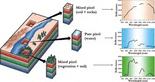
Meanwhile, unmixing - a speciﬁc instance of factor analysis - is a widely employed tool in the hyperspectral imagery literature [Bio+12; Dob+09]. In dynamic PET imaging, it can be very relevant for the extraction of factor TACs, since it directly takes into account both the nonnegativity of the data and the sum-to-one of the factor proportions that can be derived from the diﬀusion of blood in plasma and tissues. Over the last decades, cutting-edge techniques have been developed by the hyperspectral unmixing community to deal with several limitations of general blind source separation (BSS) solutions. It is the case of the homogeneity assumption embedded in the description of linear mixing models (LMM). Hyperspectral data can often present nonlinearities [NB09;Dob+14b] or spectral variability [ZH14;HDT15], which yielded new models and solutions that modify the LMM structure of standard unmixing. Moreover, as in dynamic PET, several BSS methods assume the noise to follow a Gaussian distribution. Borrowing techniques from the audio literature [FI11], a hyperspectral unmixing solution was also developed to generalize the model of the underlying noise on data [FD15].

Therefore, the main goal of this work is to develop practical contributions to dynamic PET applications that overcome the above-mentioned issues. The strategies adopted in this manuscript adapt the solutions developed in the hyperspectral literature to fit the particularities of PET data. To this end, we introduce in Chapter3a novel perturbation model that handles the variability of high-uptake tissues, often neglected in factor analysis techniques. The solution capitalizes on a previous model from the hyperspectral literature that generalizes the standard LMM with an additive spatially indexed term. The variability term is described by a previously learned dictionary and its corresponding map of coefficients. Based on a Gaussian assumption on the noise, the chosen cost function is the Frobenius norm. Then, Chapter 4 generalizes this solution to deal with different shapes of noise distribution, from Gamma and Poisson to Gaussian, including undetermined distributions in-between. This is done by means of the β-divergence. Finally, Chapter 5 presents a perspective work that benefits from the physiological knowledge inherent to parametric imaging of PET data to propose a nonlinear unmixing framework.

The work presented in this thesis has been carried out in the Institut de Recherche en Informatique de Toulouse (France), within the Signal and Communication group, in collaboration with the University of Tours and the Institut National de la Santé et de la Recherche Médicale (INSERM). This thesis has been funded by the Coordenação de Aperfeiçoamento de Ensino Superior (CAPES), attached to the Brazilian Ministry of Education, in the program “Doutorado Pleno no Exterior (DPE)”.

(23)

Introduction

Structure of the manuscript

Part I introduces the general context of this thesis and reviews the state-of-the-art methods that provide the technical basis of this work. It comprises two chapters.

– Chapter 1introduces more thoroughly the relevance of dynamic PET for clinical assessment, that is in the heart of this work. It further discusses several effects of acquisition and reconstruction affecting the quality of the final data. Finally, it presents the main challenges related to quantification and its need for a previous estimation of reference TACs or the input function.

– Chapter 2recalls the key theoretical tools and practical concepts of blind source separation applied to multivariate data analysis. After a brief review on general non-parametric methods applied in the PET literature for extraction of global TACs, it presents factor analysis as a more general alternative. Then it summarizes some of the solutions to the BSS problem and provides a brief history of factor analysis in the PET domain. Hyperspectral unmixing is subsequently detailed with its nonlinear and spectral-variability instances, preparing the reader to the developments that are to follow.

Part II gathers the contributions of this thesis to the factor analysis problem applied to the dynamic PET domain. The content of its three chapters is described hereafter.

– Chapter 3 introduces an unmixing approach to deal with the variability inherent to specific binding tissues. While factor analysis assumes the classes to be spatially homogeneous, after a careful examination of real data, we decided to propose an approach that no longer disregards possible fluctuations on the rate of tracer concentration in voxels affected by specific binding. Therefore, based on a previous perturbation model that explicitly accounts for spatial factor variability [TDT16a], we derive a formulation that allows fluctuations solely to the specific binding factor. Moreover, we constrain these variations to be described by a previously learned dictionary according to a spatial map that provides the amount of variation in each voxel of the image. The noise is considered to be Gaussian and the Frobenius norm is used to evaluate the level of fit between the data and the proposed model. The variables of this model are estimated using an optimization algorithm that ensures convergence of the iterates to a critical point, namely proximal alternating linearized minimization (PALM) [BST13]. The performance of the proposed unmixing method is evaluated on synthetic and real data. A comparison with state-of-the-art algorithms that do not take factor variability into account allows the interest of the proposed unmixing solution to be appreciated. – Chapter 4 further generalizes the approach proposed in the previous chapter to a framework that is

more adaptable to diﬀerent noise distributions. To this end, it resorts to a class of divergences that are related to a wide family of distributions that include the Gamma, Poisson and Gaussian distributions.

(24)

Introduction

This divergence is called the β-divergence. Due to its possibly nonsmooth nature, this divergence is not easily adaptable to all optimization algorithms. Therefore, we apply a majorization-minimization (MM) technique that results on multiplicative updates and that is often used to resolve this kind of problem [FI11]. A similar MM solution has also been applied to deal with nonlinearities in hyperspectral unmixing in [FD15]. We derive new updates particularly suited to the model introduced in the previous chapter. Three algorithms are then evaluated on synthetic data: β-NMF, β-LMM and β-SLMM. The β-NMF is a standard approach from the audio domain [FI11], while β-SLMM is the approach developed throughout this chapter and β-LMM is its particular instance which neglects spatial variability. Simulations are conducted on two sets of synthetic data: with and without variability. Results obtained on real data are also evaluated.

– Chapter 5introduces a more prospective work that directly relates the kinetics of specific binding tis-sues with non-specific binding ones through nonlinear unmixing. It capitalizes on data-driven parametric imaging methods [GGC01] to provide a physical description of the underlying PET data. This characteri-zation is introduced in the factor analysis formulation to yield a novel nonlinear unmixing model designed for PET image analysis. This model also explicitly introduces global kinetic parameters that allow for a direct estimation of the binding potential with respect to (w.r.t.) the free fractions in each non-specific binding tissue. As a high number of variables have to be estimated, once again the PALM algorithm is used to minimize the corresponding objective function. The algorithm is evaluated on synthetic and real data to show the potential interest of the approach.

Main contributions

Chapter 3. The contribution of this chapter lies in the introduction of a model that explicitly takes into

account the variability on the speciﬁc binding factor time-activity-curve, until now neglected in the PET liter-ature. The proposed decomposition relies on a new interpretation of the spatial heterogeneity of PET images. A joint deconvolution step is also considered in the analysis. Proximal gradient updates are computed for each variable, allowing for the inclusion of elaborate constraints [Con15] and nonsmooth penalizations. The proposed approach yields competitive performances and variability estimates on both synthetic and real data.

Chapter 4. The β-divergence is ﬁrst introduced to the PET domain. The model proposed in the previous

chapter is adapted with this flexible data-fitting term, yielding a novel algorithm. Exhaustive simulations conducted on both synthetic and real data show that optimal results for images with different reconstruction parameters may be obtained with different values of β. As a perspective, this study shows that the β-divergence has a potential interest in several steps of the dynamic PET pipeline.

(25)

Introduction

Chapter 5. This chapter introduces a new paradigm for factor analysis in dynamic PET, capitalizing on

parametric imaging. It studies the potential interest of jointly conducting nonlinear unmixing with global kinetic parameter estimation in a reference tissue compartment model framework, by considering each non-speciﬁc binding tissue as a reference. An elementary synthetic data example and a real data simulation show the promising perspective of this contribution.

(26)

(27)

Part I.

(28)

(29)

Chapter 1.

Dynamic Positron Emission

Tomography

This chapter introduces the principle and objectives of dynamic positron emission tomography (PET). It further discusses the main challenges that hamper its analysis. To this end, Section1.1provides a brief overview of PET imaging. Section1.2describes the physical properties of this imaging technique from tracer injection to acquisition of dynamic frames, while Section1.3 discusses the posterior tomographic reconstruction procedure as well as further corrections. Section1.4briefly exposes the advantages that this nuclear imaging method offers for the in vivo study of organ metabolism. General properties of both static and dynamic PET are detailed on Section 1.5. Finally, the quantification of PET images is explained in Section1.6 through the introduction of

(30)

Chapter 1. Dynamic Positron Emission Tomography

two relevant techniques: standardized uptake value and parametric imaging.

1.1. Positron Emission Tomography (PET): a brief overview

PET is a functional imaging technique that explores the physiology of organs. It is able to deliver relevant information on dysfunctions, which will precede the appearance of morphological abnormalities such as cancer and dementia, hardly detectable by anatomical imagery. The general principle of PET is the scintigraphy, which consists in injecting a radioactive tracer intravenously. The radiolabelled tracer is composed of a radioisotope attached to a molecule with specific affinity towards an organ or function within an organ. After fixation, it disintegrates emitting a positron that will be annihilated with an electron of the environment after a short course of a few millimetres. This annihilation produces two gamma photons of 511keV that leave in the same direction but opposite senses and may be detected in coincidence by the ring detectors situated around the patient, thus reporting the presence of a molecular target. The place of emission of each detected pair of photons lies on the line joining two detection points, the so-called line-of-response (LOR). When the number of detected pairs of photons is sufficient, the distribution of the radiopharmaceutical in the body of the subject can be reconstructed, using mathematical techniques or algorithms of reconstruction. This procedure provides a three-dimensional image with the quantitative information on the metabolic activity of an organ through the measure of the concentration of radiotracer in the body. Fig. 1.1shows the scheme of a PET acquisition.

In clinical PET applications, static imaging is often performed in order to obtain a map of the spatial distribution of tracer concentration. However, the best evaluation of tracer kinetics, i.e., the dynamic process of tracer uptake and retention, is achieved through the examination of changes in tracer concentration in the body over time, which prevents static imaging bias on the description of tracer metabolism [Muz+12]. In this sense, dynamic PET has received increasing attention over the last years, since it provides both spatial and temporal information about the pattern of tracer uptakes on in vivo biology. A single tracer injection allows knowledge on a large amount of information about the rate of ongoing metabolic events. Dynamic PET provides a series of frames of sinogram data with varying durations that can reach from seconds to hours. Nonetheless, as an outcome of its short acquisition intervals, especially on the earlier frames that are kept short to capture the fast kinetics right after tracer injection, dynamic PET data is highly corrupted by noise.

1.2. Physical principles of acquisition

1.2.1. Radioisotopes

Radioactivity is a natural physical phenomenon through which unstable atomic nucleus, known as radioisotopes, spontaneously transforms into more stable atomic nucleus loosing energy through the emission of radiation, such

(31)

Figure 1.1.: PET acquisition scheme

as α, β+ _{and β}− _{rays which are frequently followed by high energy photon emission or γ rays.}

Radioactive decay, which in physics corresponds to the transformation of matter into energy, occurs when the electric charge of an atom is unbalanced. The possible situations of instability are as follows:

– nucleons excess: emission of α particles;

– neutrons excess: transformation of neutron into proton, emitting electrons (β− _decay);

– protons excess: transformation of proton into neutron, emitting positrons (β+ _{decay), showed in Fig.} _1.2_.

Radioisotopes that have a positive charge excess are used as positron emitters. They are bonded with an organic molecule to form radiopharmaceuticals. The most relevant group of these compounds is the radiotracers, used in PET to diagnose abnormalities in the body tissues. We can divide them into three main categories:

– the ﬁrst one includes tracers with an excellent emission rate, but a short half-life, which is the indicator that determines the time required to reduce the radioisotope activity to the half. They can only be produced and synthesized at research centres that have a PET scan because of their short duration. Some examples: 11_O,13_{N ,}11_C;

– the second one comprises the radioisotopes with long-duration, which includes18_{F , the most used isotope}

due to its long duration. 76_{Br is also part of this group, but as it has a high positron emission kinetic}

(32)

– ﬁnally, the group with very short duration but coming from isotopic generators of very long-duration, which are used for the calibration of PET scans.

The main radiotracer used in PET is 18_{F -FDG, a glucose analog. It is obtained by replacing the normal}

hydroxyl group by the positron-emitting radionuclide ﬂuorine-18. As glucose consumption is disturbed by numerous dysfunctions, 18F_{-FDG turns out to be an excellent radiotracer for several diseases.}

1.2.2. Positron decay in PET

Due to its high positive charge, as stated previously, PET radioisotopes undergo β+ decay (Fig. 1.2), i.e., when a proton transforms into a neutron, releasing a positron β+_{(particle analogous to the electron, but with}

opposite charge) and a neutrino ν. The positron is released with a certain kinetic energy and, as it passes through the tissue, it ionizes neighboring electrons, losing energy. When resting state is reached, it combines with an electron from the tissue to form a positronium. Then, the positron-electron pair suﬀers annihilation, which releases two γ rays of 511keV in opposite sense, that is, with 180 degrees of separation between them. The principle of PET imaging is based on the detection of these two γ photons of 511keV by the PET scan crystals in order to determine the place of annihilation. An example of β+ _{emission is the decay of ﬂuorine-18}

(18_{F ) into stable oxygen-18 (}18_O):

18_F

→18_{O + β}+_{+ ν} _(1.1)

Figure 1.2.: Illustration of a β+ _{decay [}_JP05_]

Two major physical phenomena of this process negatively aﬀect the spatial resolution of the PET scan: positron range and non-collinearity of γ rays.

– Positron range: The event of annihilation does not detect the emission of the positron itself. After emission, the positron follows a dentition trajectory through the tissue and interacts with it through ionization. There is a distance between annihilation and decay that is called free-course and depends on the initial energy of the positron and the composition of the tissue, in particular its density. For low-energy positron emitters, this distance in soft tissues is small (for instance, 0.5 mm for the18_{F ). For high-energy}

positron emitters, it will highly aﬀect resolution.

– Non-collinearity of γ rays: For a positron to combine with an electron from the tissue, it must lose all its energy and have the same kinetic energy as that due to the tissue temperature. Although the

(33)

positronium is at the same temperature as the tissue, its angular momentum is not negligible, since photons have little angular momentum compared to energy and they must maintain the same momentum of the positronium. If the positronium is moving in the same direction as one of the photons, this photon will have more energy than the other, but generally this effect does not significantly affect PET scan detection. If the positronium is moving in a direction perpendicular to the annihilation photons, due to conservation of momentum, they will be slightly non-collinear (non-collinearity is, in average, typically of the order of less than 1 degree), resulting in a loss of resolution of 1 to 2 mm. Fig. 1.3 illustrates this process.

Figure 1.3.: Non-collinearity due to conservation of the momentum. [JP05]

Radioisotopes with excess of protons may also decay by electron capture, but these will not be detected by a PET scan. To disintegration by β+ _{decay, the isotope needs to have at least 1,02MeV more energy than the}

isotope for which it decays.

1.2.3. Coincidence detection

If two detectors on opposite sides of the patient detect an event at about the same time, then annihilation occurred somewhere along the straight line between the detectors, as illustrated by Fig. 1.4. This straight line is called the LOR. The key to PET acquisition is precisely the ability to identify these coincidental events.

Figure 1.4.: Detection of positron annihilation

In order to detect the simultaneous arrival of the two γ rays in opposite directions, it is essential to have two detectors on opposite sides of the patient in all directions. Therefore, detectors are usually constructed as

(34)

annular arrays of small crystals that are placed around the patients, as showed in Fig. 1.4. The area deﬁned by crystals where annihilation occurs is tubular (and not simply a line). In analog systems, each detector is formed by a scintillation crystal and a photomultiplier1_{. Detection is then performed if the two γ rays arrive}

at the same time with the same energy. In this case, simultaneity is deﬁned by a coincidence circuit, which is based on two windows:

– the temporal window: is usually in the range of 5 to 16 ns. In practice, when the ﬁrst photon is detected, the time window is started and remains open for a given time τ . Every photon detected while the time window is open will be associated with the ﬁrst photon. A new pair of photons can only be detected after the window is closed.

– the energy window: detects photons with an energy comprised within a range with mean value of approximately 511eV. It is useful to neglect the arrival of photons from scattering, which have a lower energy and prevent pile-up eﬀects in which the crystal receive energy from several photons.

Several phenomena directly aﬀecting image resolution can be identiﬁed:

– True coincidences: when two photons of the annihilation event are detected by crystals in opposite directions as a photopick;

– Scattered coincidences: when one of the photons goes through a Compton eﬀect, altering its LOR due to the interaction of a γ ray with an electron of the tissue;

– Random coincidences: when two photons from diﬀerent annihilations are detected as originating from the same annihilation.

The interaction of photons entering the detectors with electrons from the crystal occurs either through the photoelectric effect, where the full photon energy is transmitted to the crystal, or through the Compton effect that, due to its scintillation, only transmits part of the energy. The light energy generated is then transferred to the photocatode of the photomultiplier tube through a light guide. The role of the photocatode is to transform the light energy into electrons that are directed to the first dynode to be multiplied by the factor of secondary emission. The signal coming out of the photomultiplier provides a measurable electrical impulse whose integral is proportional to the energy of the photon that has entered the crystal. During the integration time, which depends on the rate of light decrease in the crystal, the detector is not able to measure another event. This phenomenon, called dead time, is responsible for losses in sensitivity to high counts. In general, the density, as well as the energetic and temporal resolutions, affects the performance of different PET imaging devices.

1_{Recently, digital PET detectors were developed to overcome the limitations of conventional photomultiplier technology. This}

topic will not be further detailed in this work for brevity purposes.

(35)

Figure 1.5.: Illustration of annular arrays of small crystals [JP05]. View of a PET scanner from the annular plane (left) and view along the axis of the scanner (right).

1.2.4. Time-of-flight

The photons released during the course of a PET scan reach the detectors at almost the same time. The key to understand the concept of time-of-flight (TOF) relies on the “almost”. TOF is the time difference between the detection of photons released during coincident events. The measurement of the difference in arrival times allows to more accurately identify the location of the annihilation event along the line between the two detectors. With TOF PET scanners then, each event is more informative. The key limitation to building a TOF scanner is the time taken by the scintillation process within the crystals.

1.2.5. Photon-tissue interaction

Before reaching the detector, the photons pass through the patient and some of them interact with the tissue. There are three possible interactions between the 511keV photons and the tissue: the photoelectric eﬀect, the Compton eﬀect and the Rayleigh scattering, which are shown in Fig. 1.6

– Photoelectric effect: In the photoelectric eﬀect, the photon is completely absorbed by an electron from the atom, overcoming the binding energy and releasing the electron with kinetic energy corresponding to the rest of the photon energy. This phenomenon usually happens with low-energy photons and high atomic number atoms.

– Compton effect: In the Compton effect, or incoherent scattering, the annihilation photon interacts with an electron from an upper layer. The photon loses a part of its energy and is dispersed in a new direction, while the electron leaves the valence layer. The Compton effect contributes to the attenuation of γ rays. The effect of the Compton diffusion on the final resolution of the PET image depends on several instrumental considerations of the machine.

– Rayleigh scattering: Rayleigh dispersion or coherent dispersion occurs when a photon bounces the atoms in the matrix without causing ionization. The photon changes direction and there is therefore a change in the moment, which is transferred to the atoms of the matrix. However, such dispersion is not frequent at 511 kV in the tissue and can be ignored.

(36)

Figure 1.6.: Eﬀects of the interaction of radiation with matter [JP05]

Due to the small angle of the scattered photons, the apparent attenuation may be smaller than the actual attenuation. The coefficient of the apparent attenuation depends on the geometry and the energy resolution of the system. Actual attenuation can be measured with experimental configurations that exclude almost all dispersed photons. A closely collimated, i.e. directed, source and detector allow only non-scattered photons to reach the detector. In some cases, the attenuation coefficient serves as the input parameter used during reconstruction. A lower value than the actual value can be used to account for small angle dispersion.

1.3. Reconstruction and corrections

1.3.1. Reconstruction process

PET data is constructed through the projection of the location of coincidences occurring within the object of study (e.g., an organ). Therefore a step of tomographic reconstruction becomes essential to recognize the object from its projection.

Data arrangement into a sinogram

The elementary PET data are the LORs connecting a pair of detectors that are placed in coincidence. The coincidences recorded on each LOR may be arranged in a matrix called sinogram. Each row of this matrix corresponds to a diﬀerent angle of the one-dimensional projection. The number of columns is equivalent to the number of LORs for each measurement angle. Sinograms may have, for instance, 256 rows of measurement angles while 192 pairs of detectors for an angular position. Each element of the sinogram represents a LOR between two detectors.

Figure1.7shows two detectors d1and d2connected by an LOR that corresponds to a point of the sinogram.

The sum of the coincidences detected within this LOR is allocated in the position deﬁned by s1 and φ1. Each

event accepted by the coincidence circuits adds a unity to the total value of this point of the sinogram.

(37)

Figure 1.7.: Line-of-response (right) and point correspondent to the LOR in a sinogram (left) [Rey07]

PET data corresponding to one acquisition time may be of two or three dimensions. In “2D” mode, the system only registers the coincidences occurring between two crystals belonging to the same ring or two neighboring rings. To this end, the scanner is equipped with septa between the detection rings in order to stop annihilation photons whose direction correspond to a high copolar angle. In “3D” mode, the LORs are not only in the axial plane, but also at a considerable angle to these planes and for each angle there is a stack of planes.

Reconstruction methods

After detection and allocation of coincidences, the next step consists of computing the radioactivity distribution within the ﬁeld of view (FOV) with the information recorded in the sinogram. There are two main techniques of reconstruction: ﬁltered back-projection and iterative reconstruction.

– Filtered back-projection: This method is generally applied aiming to implement Fourier reconstruction. The first step of the algorithm consists on filtering each line of the sinogram with a ramp filter that is generally combined with a low-pass filter to prevent noise amplification. Then the method proceeds to the backprojection of filtered projections for each different measured angle. The major advantages of this method are its speed, low complexity and good performance when tracer binding is rather homogeneous. On the other hand, it amplifies the statistical noise of the acquired data.

– Iterative reconstruction: Iterative algorithms are initialized with a random estimation of the solution and iteratively proceed to the reconstruction and projection operations. Reconstruction consists of ac-quiring a frame of the image from the sinogram. The inverse operation, i.e., calculating the sinogram of a given frame, is called projection. In each iteration, the projection of the current solution is compared to the measured projection. The error between those two is supposed to decrease in the next iteration and

(38)

the process continue until this error is smaller than a previously deﬁned criterion, meaning the algorithm has converged. Iterative reconstruction allows a more robust modelling of the eﬀects occurring in the PET scan and therefore is more general than Fourier reconstruction. However, it presents a high computational cost and, consequently, is much slower than the latter one. Nonetheless, this drawback has been overcome by our current computational resources that allows the use of these algorithms for clinical practice. The preferred iterative algorithms for reconstruction are based on expectation maximization (EM). The most frequently used method accelerates EM by an ordered subset, corresponding to the acronym OSEM.

1.3.2. Standard corrections

Several coincidences are detected in PET image acquisition, but just a few hold relevant information about the place of annihilation as stated in Section1.2.3. Furthermore, the interaction of the photon with the tissue (detailed in 1.2.5) when passing through the patient before getting to the detector attenuates the signal. In order to correct the deteriorated signal, diﬀerent strategies were proposed. Some examples of corrections are described in the following.

Attenuation correction

Attenuation occurs when the emitted photons are absorbed before reaching the detector. In a PET scan, it is mainly due to the eﬀects presented in Section1.2.5. Attenuation correction is then applied to obtain a more realistic representation of the radiotracer distribution from the obtained deteriorated information.

Attenuation correction is easily modeled along a line, knowing the linear attenuation coefficient at each point of space and for an energy of 511keV. Once these parameters are known, it is sufficient to calculate the integral of the attenuation coefficient along each LOR. To this end, a projection step is performed through an image of the attenuation coefficient, in order to compute the set of corrective factors corresponding to these integrals (one by LOR). Whatever the point of annihilation of the coincidence detected along the line joining the two crystals, the total distance traveled by these two photons is the same. The amount of attenuating material traversed is, therefore, the same. Thus, attenuation on an LOR does not depend on the location of annihilation. The main challenge when applying this method of correction relies on the determination of the set of linear attenuation coefficients. In practice, a mean coefficient for each voxel of the reconstructed image is defined and an image of the linear attenuation coefficients is produced. This image is often called attenuation map. This map is measured by means of an acquisition in transmission carried out either by a computed tomography (CT) scanner or by an external source emitting 511 keV annihilation photons. Currently, most PET scans are coupled to a CT scanner that estimates the attenuation coefficients for given values of photon energy. The final attenuation map is obtained by converting it to correspond to 511keV.

(39)

Scatter and random correction

In a clinical PET scan conditions, the eﬀects presented in Section 1.2.3 are an important source of inaccu-racy. To reduce these negative eﬀects, some techniques were developed for correction of random and scattered coincidences.

– Correction of random coincidences: There are two most currently used methods to estimate the distribution of random coincidences and its variants. The ﬁrst method uses the measurement of the count rate of events detected by each crystal. It therefore assumes that the tomograph is able to record these data. At the end of the acquisition, an estimation of the number of random coincidences per LOR is inferred from the number of events detected by each crystal of the LOR within a coincidence window. This method has two disadvantages: in most cases, it overestimates the amount of random coincidences, and it does not take into account the characteristics of the coincidence detection chain (dead time and multiple coincidence processing). In addition, event rates may vary throughout the acquisition. A second eﬀective and simple way of avoiding random coincidences is through temporal windows, as described in Section 1.2.3. The advantage of this method is that the estimate of random coincidences has exactly the same characteristics as the raw coincidences [Stu10].

– Correction of scattered coincidences: The correction of scattered coincidences has been explored in many works. The first category of methods assumed that after correction of all phenomena except scatter-ing, the coincidences detected outside the patient or object are scattered coincidences. The contours of the patient or object are either obtained directly via CT, if available, or estimated from a first reconstruction of the PET data after correction for attenuation and random coincidences. Since the distribution of the scattered coincidences is a low frequency signal, the tails of this distribution are measured outside the patient or the object in the sinograms and then completed by adjustment with different functions in order to estimate the distribution of the coincidences scattered inside the patient or the object (always in the sinograms). A second category of methods explores the fact that only the events detected around 511keV are of interest. It is based on energy windowing, as detailed in Section 1.2.3. The challenge in this case is to determine whether a low energy received is due to the limited energy resolution of the crystals, or to a hypothetical previous scatter. Many other methods were proposed in the literature that will not be detailed in this review but can be consulted in [Stu10].

1.4. Dynamic PET imaging

Dynamic PET imaging consists of acquiring a series of static PET images in diﬀerent frame durations after the injection of the radiopharmaceutical, followed by its reconstruction. The frames of time may vary according to