Any correspondence concerning this service should be sent
to the repository administrator: [email protected]
This is an author’s version published in:
http://oatao.univ-toulouse.fr/19167
To cite this version:
Mathieu, Bérengère and Crouzil, Alain and
Puel, Jean-Baptiste Interactive segmentation: a scalable
superpixel-based method. (2017) Journal of Electronic Imaging, 26 (6). 1-18.
ISSN 1017-9909
Official URL
DOI :
https://doi.org/10.1117/1.JEI.26.6.061606
Open Archive Toulouse Archive Ouverte
OATAO is an open access repository that collects the work of Toulouse
researchers and makes it freely available over the web where possible
Abstract. This paper addresses the problem of interactive multiclass segmentation of images. We propose a fast and efficient new interactive segmentation method called superpixel α fusion (SαF). From a few strokes drawn by a user over an image, this method extracts relevant semantic objects. To get a fast calculation and an accurate segmentation, SαF uses superpixel oversegmentation and support vector machine classification. We compare SαF with competing algorithms by evaluating its performances on reference benchmarks. We also suggest four new datasets to evaluate the scalability of interactive segmentation methods, using images from some thousand to several million pixels. We conclude with two applications of SαF.
DOI: 10.1117/1.JEI.26.6.061606
Keywords: image analysis; interactive segmentation; superpixel; graph-factor; support vector machine; dataset; image editing
1 Introduction
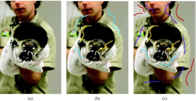
Image segmentation is still a challenging research topic in the image analysis community. Its goal is to group similar and neighboring pixels in order to partition the image into structures corresponding to coherent elements. However, depending on the application context, even for the same image, the term “coherent elements” can have different meanings. An example is given in Fig.1, which shows for the same image two possible segmentations. In the first case, we want to select only the main character, for example, to copy and paste it on another background. In the second case, we are interested in some details, like the clothing.
This example illustrates the complexity of finding a seg-mentation algorithm able to deal with the variety of contexts of use. During the last decade, convolutional neural networks (CNNs) had led to significant advances in the semantic seg-mentation task.1–3However, even if results of CNN methods
are impressive, it is not yet possible to correct errors of the produced segmentation and, to the best of our knowledge, the user input can be used4only during the training stage. Even if the output of a CNN can be used as the input of an optimization process constrained by the user input, it requires an extensive dataset for training. Currently, we think that there is always room for interactive methods with an iterative process allowing the user to correct errors of the method and to achieve any desired segmentation. For each image, according to his needs, the user can change the object categories and the level of details. Basically, the user chooses some pixels (named seeds) and indicates for each of them the element to which it belongs. Additional constraints about the wanted segmentation are deduced by analyzing these seeds. Adding or removing some seeds can improve the produced result.
The two most common application scopes for these kinds of algorithms are segmentation of a particular anatomic
structure in medical imagery5–14 and natural photograph (such as an image taken with a smartphone or a camera) manipulation for art or graphic design purpose.15–26These two application scopes correspond to distinct problems, with substantial differences among proceeded image features and the available prior information. Thus, in the scope of this paper, we focus only on interactive segmentation to select one or several objects in natural photographs.
1.1 Previous Work
Currently, several interactive segmentation methods solve only binarization problems by separating a desired fore-ground object from the backfore-ground. These methods may be boundary-based21–23 or region-based.15–20,24–28Figure 2 shows the most common way to give seeds, related to each category.
In boundary-based methods, the user provides landmark points and the algorithm links them with a closed curve, which satisfies both regularization and edge evidence constraints. The combination of piecewise-geodesic paths (CPP) is one of the most recent boundary-based interactive segmentation methods. Proposed by Mille et al.,21 this algorithm generates several relevant paths and selects the one minimizing an energy function that decreases when the path has a high probability to be on an image edge, when the regions inside and outside the path are homo-geneous and when the path contains few self-overlaps and self-intersections.
In region-based methods, the user gives seeds by drawing strokes on the objects. Pixels are grouped to form regions, according to the similarity to object models created by the seeds. The interactive graph cuts (IGC) algorithm, proposed by Boykov and Jolly,16operates by minimizing an energy function E grouping hard constraints (seeds provided by user interaction) and soft constraints (similarities between pixels in spatial and intensity domains). To find the
*Address all correspondence to: Alain Crouzil, E-mail:[email protected]
Interactive
segmentation: a scalable superpixel-based
method
Bérengère Mathieu,aAlain Crouzil,a,*and Jean-Baptiste Puelb
aUniversité Toulouse III, Institut de Recherche en Informatique de Toulouse, Toulouse, France
segmentation S , which minimizes E, Boykov and Jolly16 used a fast min-cut/max-flow algorithm on the graph G¼ hV; Ei with:
• V¼ Vp∪ Vt, where:
– Vp¼ fv1; : : : ; vng is a set of nodes such that each
pixel pi is linked to a node vi;
– Vt¼ fT; Sg is a set grouping two particular
nodes: the sink T and the source S; • E¼ Ep∪ Et, where:
– Ep is the set of edges linking Vp nodes, under
a standard 4- or 8-neighborhood system; – Etis the set of edges linking each node in Vp to
each node in Vt.
Each edge is weighted such that Epedges have a strong
weight if the two linked nodes correspond to similar pixels and Etedges have a high weight if the Vpnode has a strong
probability to belong to the foreground when the second node is the source and to the background when the second
node is the sink. The method of Boykov and Jolly16obtained very good results in the McGuinness interactive segmenta-tion review,29 but it solves only a binary classification problem.
In the McGuinness et al. review,29the interactive seg-mentation method using binary partition trees (BPT) of Salembier et al.25 is the main challenger of IGC. Starting from a hierarchical segmentation of the image represented as a BPT, the algorithm produces a binarization by merging regions. First, according to the seeds given by the user, some leaf nodes of the binary tree are labeled. Then, these labels are propagated to the parent nodes, until a conflict occurs when the two children of a node have different labels. In this situation, the parent node is marked as conflicting. Finally, all nonconflicting nodes propagate their labels to their children. At the end of this stage, some subtrees can remain unlabeled. These unclassified regions are labeled with the label of a previously classified adjacent region. When several adjacent regions with different labels are candidates to label the unclassified region, the closest one according to the Euclidean distance is chosen.
The simple interactive object extraction proposed by Friedland et al.17uses seeds to generate color signatures30
(a) (b) (c)
Fig. 1Two segmentation results of the same image. (a) Original image, (b) a coarse segmentation, and (c) a finer segmentation.
(a) (b) (c)
Fig. 2User interaction for the different categories of interactive segmentation methods. (a) Boundary-based, (b) region-Boundary-based, and (c) region-based multiclass interactive binarizations.
of background and foreground, represented as a weighted set of cluster centers. The distances between each remaining pixel and any of these centers are computed. The pixels are merged with the region including the closest cluster.
To the best of our knowledge, the last proposition of an interactive region-based binarization method is the segmen-tation algorithm of Jian et al.31 using adaptive constraint propagation (ACP). First, the image is segmented using the mean-shift method. Then, features of corresponding regions are extracted. During the following step of ACP, pair-wise constraints are generated by analyzing the given seeds. Next, ACP is performed in order to learn a global discrimi-native structure of the image. This structure allows finally assigning each region to the background or the foreground. The seeded region growing (SRG) algorithm, proposed by Adams et al.,15the interactive multilabel segmentation (IMS) method of Santner et al.,26 the robust IMS with an advanced edge detector (RIMSAED) of Müller et al.,28 and the robust interactive image segmentation (RIIS) of Oh et al.32are attempts to solve the multiclass interactive seg-mentation problem.
The method of Adams and Bischof15 is a very simple recursive method, where regions are characterized by their average color. The initial regions begin with the pixels labeled by the user. Then, the regions are grown by including the adjacent pixels with the most similar color. The average colors are updated and the algorithm iterates until all the pix-els have been grouped. In spite of its speed, this algorithm suffers from the simplicity of its region color model.
The IMS algorithm26has two major steps. First, the pixel likelihood to belong to each class is computed thanks to a random forest (RF) classifier. Then, an optimal segmentation is found by minimizing an energy function that linearly combines a regularization term and a data term
EQ-TARGET;temp:intralink-;e001;63;378 E¼1 2 XN i¼1 PerDðEi; ΩÞ þ λ XN i¼1 Z Ei fiðxÞdx; (1)
where Ω is the image domain, Eiare the N pairwise disjoint
sets partitioning Ω, PerDis a function encouraging to have
smooth boundaries following pixels with high gradient value, and fi is the output of the RF classifier. During the
first stage, color and texture descriptors of pixels are com-puted. Santner et al.26compared several features and showed that the combination of Lab color space and local binary pattern texture descriptor gives the best results. Next, the classifier is trained with the seeds. The trained classifier gives for each pixel the likelihood to belong to each class. These likelihoods are used during the second step, into the data term. The regularization term penalizes the boundary length, avoiding noisy segmentation. Santner et al.26 formu-lated the segmentation problem like a Potts model and solve it using a first-order primal-dual algorithm. However, this method is rather slow. Santner et al.26proposed a massive parallelization and a GPU implementation of IMS, segment-ing an image of 625 × 391 pixels into four classes on a desk-top PC featuring a 2.6-GHz quad-core processor in about 2 s. The RIMSAED method of Müller et al.,28similarly to IMS method, minimizes Eq. (1). Nevertheless, in the RIMSAED algorithm, the term PerD does not simply use
gradient magnitude but a more accurate edge detector,33 which incorporates texture, color, and brightness. The data
term depending on fi uses color and location distributions
of seeds to deduce the likelihood of a pixel to belong to each class. This approach is similar to the one used by Nieuwenhuis and Cremers.34 The contribution of Müller consists of using potential functions that allow the segmen-tation method to correct wrong seeds by introducing a prior probability of seeds to be erroneous.
For their proposed method RIIS, Oh et al.32used occur-rence (capturing global distribution of all color values within seeds) and cooccurrence (encoding a local distribution of color values around seeds) probabilities to detect and exclude the erroneous seeds. Occurrence and cooccurence probabil-ities are computed using a histogram of gray level values of seeds. They produce a confidence score for each seed. The final segmentation is obtained by minimizing an energy similar to the one used by Boykov and Jolly16The energy function contains a data term that checks the homogeneity of resulting regions as well as the consistency with seeds. It also integrates a regularization term encouraging similar pixels to be merged. As RIIS has a regularization term adopt-ing a nonlocal pairwise connection by computadopt-ing k-nearest neighbors (k-NN) in the feature space, an approximation of the optimal solution is found using sparse solvers.35 1.2 Contributions
The main contribution of this paper is an interactive multi-class segmentation method, named SαF. The SαF algorithm achieves results similar to or better than state-of-the-art methods, while keeping a low algorithmical complexity that allows it to correctly segment images having millions of pixels.
The computation of an accurate segmentation is ensured by formulating the interactive segmentation problem as a discrete energy minimization problem, given in the form of a factor graph.36Notably, we propose a regularization term that significantly reduces the required number of seeds while allowing the correct segmentation of small objects belonging to rare classes. The consistency of the segmentation result regarding the image visual features and the seeds given by the user is obtained by a supervised learning stage.
The efficiency and the scalability of SαF are ensured by an oversegmentation initialization step. Oversegmentation is the task of grouping pixels into small homogeneous regions, called superpixels. During the last decade, a lot of methods have been suggested and a recent review37shows that five of them achieve similar results. By providing a new evaluation benchmark of photographs of several million pixels, we point to unexpected difficulties encountered by these meth-ods and justify the use of the simple linear iterative clustering (SLIC) algorithm in SαF.
We evaluate SαF with state-of-the-art benchmarks and we quantitatively analyze its scalability by creating and making available four new datasets with, respectively, big images (1800 × 1201 pixels), medium images (1350 × 901 pixels), small images (1013 × 675 pixels), and tiny images (500 × 334 pixels). We provide an implementation of SαF as a Gimp plugin and we use SαF in a landscape teaching Android application.
In the following sections, we will first explain the mod-eling of the interactive segmentation problem as a discrete optimization problem, represented by a factor graph. Then, we will describe experiments to choose components that
are now parts of SαF and how we configure those compo-nents. Finally, we will evaluate its performance by compar-ing it to the height of state-of-the-art methods, against three different benchmarks. We will conclude with two examples of applications.
2 Interactive Segmentation as a Discrete Optimization Problem
Let X¼ fx1; : : : ; xMg be a partition of an image I in M
nected components. In the case of SαF algorithm, these con-nected components are small sets of similar pixels, called superpixels. Computing a multiclass segmentation of I means to assign to each superpixel xi a label λj related to
the class j. Usually, λiis a positive integer and for K classes,
the set of labels that may be given for a region is Λ ¼ fλ1; : : : ; λKg. In the case of interactive segmentation,
K is deduced by analyzing the number of colors used by the user when drawing the seeds.
Let G¼ hX; Ei be an undirected graph, where X is the set of vertices (one vertex by superpixel) and E is the set of edges, linking each pair of superpixels containing adjacent pixels. Let c¼ fc1; : : : ; cNg be a set of random variables,
indexed by the vertices of G, such that ci∈ Λ. We assume
that G is a Markov random field (MRF). Thus, we can find an optimal segmentation c of the image I by minimizing
EQ-TARGET;temp:intralink-;e002;63;476 EMRFðcjIÞ ¼ exp " XN i¼1 fdataðx i; ciÞ þ X ðxi;xjÞ∈E ωðxiÞfregðxi; ci; xj; cjÞ # ; (2)
where fdatais a data term, fregis a regularization term, and ω
is a weighting function. The following optimization problem can be easily modeled by a factor graph, which represents the structure of the underlying problem in a more precise and explicit way than MRF can.38
A factor graph G0¼ hX0; F0; E0i is a bipartite graph
representing the factorization of a function of M variables, gðx1; : : : ; xMÞ, by
• X0a set of vertices denoting the M variables; • F0a set of vertices related to the decomposition of g in
subfunctions called factors;
• E0is the set of edges linking each factor to its related variables.
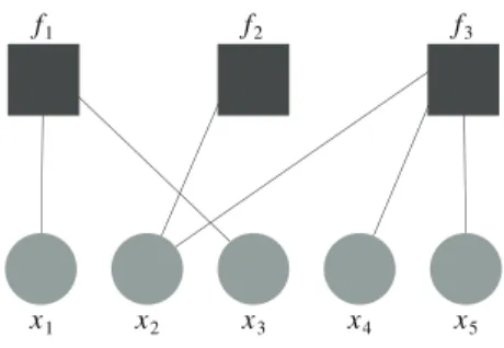
Figure3shows the concept of factor graph.
In the case of Eq. (2), the factorization is straightforward
EQ-TARGET;temp:intralink-;e003;326;741EFG¼ YN i¼1 Idataðx i; ciÞ Y ðxi;xjÞ∈E Iregðx i; ci; xj; cjÞ; (3) where Idataðx
i;ciÞ ¼ exp½fdataðxi;ciÞ- and Iregðxi;ci;xj;cjÞ ¼
exp½ωðxiÞfregðxi;ci;xj;cjÞ-.
2.1 Data Term
Let X¼ hXG; XCi be a partition of X into two sets: XG for
the superpixels containing seeds of only one class and XCfor
the superpixels that do not contain seeds or contain seeds of several classes. The set XGallows computing the probability
pðλjjxiÞ for the superpixel xito belong to the class of label
λj. As we want to minimize Eq. (3), the data term is given by
EQ-TARGET;temp:intralink-;e004;326;575f dataðx
i; ciÞ ¼ 1 − pðλjjxiÞ; where ci¼ λj: (4)
For multiclass classification problems, the second approach of Wu et al.39is well known to give a satisfactory approximation of the probability of a variable to belong to a given class, using the result of a supervised learning method. This algorithm has been tested both with a support vector machine (SVM) and a RF. Section 3.3 explains how we empirically chose one of them to compute the data term.
2.2 Regularization Term
The segmentation result obtained from the minimization of fdatacould be very noisy, with isolated superpixels having a label different from its neighbors. On one hand, removing this noise by adding seeds is a tedious task and degrades the user experience. On the other hand, a regularization term encouraging large and compact regions can remove rare classes corresponding to small objects.
In this paper, we propose a regularization term freg,
designed to increase spatial consistency of given labels while preserving rare classes. In a segmentation result, let xnbe a noisy superpixel (i.e., a superpixel with an erroneous
label) and xra superpixel of a rare class. Both xnand xrhave
a majority of neighbors with different labels. Let λn be the
label of xnand λr the label of xr. The fact that a superpixel
has the label λrand several adjacent superpixels with labels
different from λris more common than the fact that a
super-pixel has the label λnand several neighbors with labels
differ-ent from λn. Figure4shows an example where superpixels in
blue (the rare class) are more likely adjacent to superpixels in black than to superpixels in pink. In other words, the prob-ability for a superpixel in blue to have neighbors in black is higher than the probability for a superpixel in pink to have neighbors in black. By estimating these two probabilities, we can distinguish between correctly labeled superpixels belonging to rare classes and noise.
The steps for the computation of the regularization term are the following. First, SαF produces a preliminary segmen-tation, by assigning to each superpixel the most likely label, according to the result given by the supervised learning method used in the data term estimation. This segmentation is analyzed to compute for each class i, piðjÞ is the
proba-bility for a superpixel of class i to have a neighbor of class j, where j∈½1; K-.
f1 f2 f3
x1 x2 x3 x4 x5
Fig. 3Factor graph modeling the factorization: F1ðX1; X2; X3; X4; X5Þ ¼ f1ðX1; X3Þf2ðX2Þf3ðX2; X4; X5Þ.
The regularization term is finally given by
EQ-TARGET;temp:intralink-;e005;63;515
fregðxi; ci; xj; cjÞ ¼ 1 − max½piðjÞ; pjðiÞ-: (5)
2.3 Weighting Function
Weighting function ω allows balancing the influence of the regularization term with respect to the data term. Unlike pixels, superpixels have varying numbers of neigh-bors. The influence of the regularization term depends on this number and the weighting function should include it. After several tests on a subset of state-of-the-art benchmarks (see Sec.4), we empirically choose the following weighting function: EQ-TARGET;temp:intralink-;e006;63;369 ωðxiÞ ¼ 0.7 jneiðxiÞj ; (6)
wherejneiðxiÞj is the number of neighbors of superpixel xi.
2.4 Inference Method
Due to the number of possible segmentations, the search of the one minimizing Eq. (3) is not realistically feasible. Following the conclusions of Kappes et al.36for image analy-sis problems with superpixels, we use a generalization of the α expansion algorithm of Boykov et al.,40the α fusion algorithm, with the fusion-moves and the order-reduction of Fix et al.41
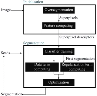
2.5 Algorithm Overview
Figure5shows an overview of the proposed SαF algorithm, which can be divided into an initialization stage extracting image features and a segmentation stage taking seeds into account.
We consider an image I that must be segmented. During the initialization step, SαF groups pixels of I into N super-pixels. As explained above, superpixels are small homo-geneous color regions, significantly less numerous than pixels. Thus, using them as visual primitives instead of pixels significantly reduces the execution times of the next algo-rithm steps. In the context of SαF algoalgo-rithm, superpixels
are used as an image compression tool. Their features are extracted to produce a set P of N vectors.
The segmentation stage of SαF is iterative: as long as the user adds or removes seeds, the segmentation is updated. We start by analyzing seeds provided by the user to deduce K, the number of classes. We create a set of Kþ 1 labels f0;1; : : : ; Kg with 1; : : : ; K the labels representing each class and 0 a void label. So, we can assign to each pixel pa label j such that j > 0 if p is a seed or j¼ 0 otherwise. Then, for each class, we create Sj, the set of superpixels
including at least one pixel with label j and the others with label j or 0. Next, we train a classifier for multiclass classification, using, for each class j, the features of the superpixel set Sj. Finally, we compute data and
regulariza-tion terms as explained in Sec.2and we use α fusion algo-rithm to find an optimal labeling of the superpixels. The label given to each superpixel is assigned to each pixel belonging to it, producing the segmentation.
(a) (b)
Fig. 4Problem of the distinction between rare classes and noise in segmentation. (a) Image with three classes, two dominant classes (in black and pink), and one rare class (in blue). (b) Example of a noisy segmentation. Boundaries of superpixels are in white.
Data term computing
Initialization Seeds Superpixel descriptors Segmentation Image Segmentation Oversegmentation Feature computing Superpixels
Data term computing Classifier training Optimization First segmentation Regularization term computing Data term computing
3 Experiments to Select and Tune SαF Components 3.1 Oversegmentation
Superpixels are the results of an oversegmentation of the image: boundaries of objects in the image should match superpixel boundaries, but the same object can be partitioned into several superpixels. In the context of interactive segmen-tation, a good oversegmentation algorithm must produce as few superpixels as possible and make as few object overlap-ping errors as possible, because they cannot be corrected by the next steps of the algorithms. Unfortunately, reducing the number of superpixels requires increasing their size and, by grouping more and more pixels into a same superpixel, the probability of errors increases dramatically. Moreover, the superpixel extraction has to be fast, avoiding that this preprocessing step slows down the whole method.
According to the Stutz review,37Felzenszwalb algorithm (FZ),42quick shift (QS),43entropy rate superpixels (ERS),44 SLIC,45and contour relaxed superpixels (CRS)46outperform other oversegmentation algorithms. In addition, all these methods achieve similar results in both precision and execu-tion time. However, the datasets used by Stutz contain only small images (some thousand pixels). To check that these algorithms remain competitive when dealing with big images (several million pixels), we provide a heterogeneous size image dataset (HSID), containing 100 images and the corre-sponding ground truth.
We evaluated FZ, QS, ERS, SLIC, and CRS as well as the two most recent oversegmentation methods: algorithm of Rubio et al. [boundary-aware superpixel segmentation (BASS)]47and waterpixel (WP)48algorithm. We use imple-mentations made available by their authors.
To quantify superpixel boundary adherence, we adapt the common boundary recall measure, using fuzzy-set theory to introduce some tolerance error near the border pixels
EQ-TARGET;temp:intralink-;e007;63;366 FBRðS; GÞ ¼ 1 jBGj X p∈BG exp & −dðp − p 0Þ2 2σ2 ' ; (7)
where G is a ground truth, S is the oversegmentation result, BGis the set of boundary pixels in G, BSis the set of
boun-dary pixels in S, dðp − p0Þ is the distance between p and p0,
the nearest boundary pixel in S, p0¼ arg min
pj∈BS
½dðp − pjÞ-.
The bandwidth parameter σ regulates the sensitivity to the error by penalizing more or less the pixels far from the boundary. According to McGuinness et al.,29we set it to 4. We made seven tests where methods are configured to, respectively, produce about 500 (test 1), 700 (test 2), 900 (test 3), 1100 (test 4), 1300 (test 5), 1500 (test 6), and 1700 (test 7) superpixels (Figs.6and 7).
Figure6shows the evolution of FBR scores with respect to the number of superpixels. The evolution of the execution time is given in Fig.7.
Results show that QS, BASS, CRS, and WP fail to cor-rectly oversegment HSID images. Algorithms FZ, SLIC, and ERS achieve similar boundary adherence with an equivalent number of superpixels, but ERS and FZ are significantly slower than SLIC. As the execution time is critical for an interactive segmentation method, we chose to use SLIC.
The HSID dataset and the complete results of the evaluation are available at Ref. 49. They are described in a previous paper.50
3.2 Descriptor
We describe each superpixel by its normalized average RGB color and the normalized location of its center of mass. We made additional tests with Lab color space and obtained results similar to those achieved with RGB. As converting a pixel from RGB to Lab color spaces requires extra com-putation, we chose to use only RGB color space.
This simple descriptor has the benefit of being quickly computed and used. In addition, as explained in Sec. 4.4, color and location are intuitive concepts for the user and make the behavior of SαF easily predictable.
However, some previous works (for example, the method of Gould et al.51) show that texture information from super-pixels is often also valuable. Thus, we designed another version of SαF with color, location, and texture features. As a texture descriptor, we used uniform local binary pat-terns (LBP-U),52 which have been successfully integrated Fig. 6 Boundary adherence evolution (FBR) with respect to the number of superpixels.
Fig. 7 Execution time evolution with respect to the number of superpixels.
in many applications.26We evaluated it with the seven data-sets and their related metrics presented in Sec. 4. While the computation of LBP-U represents only 23% of the total execution time of the initialization stage, the impact of the addition of a texture descriptor in the segmentation stage is more significant, taking 76% of the total execution time. The segmentation stage occurs each time the user updates the seeds, and this result led us to discard the LBP-U version of SαF.
Moreover, on all the tested datasets, we did not find any evidence that LBP-U information can improve accuracy or allow reducing the number of required seeds. Because in SαF the SLIC oversegmentation algorithm is tuned to produce very small regions (about a few hundred of pixels) with homogeneous colors (average standard deviation for each color channel is about 4%), this result is not surprising.
3.3 Classifier
We evaluated the accuracy of probability distribution pre-dicted by two different classifiers integrated in the approach of Wu et al.: an RF and an SVM. For RF, we used the ALGLIB implementation.53 Two parameters, the number of decision trees and the percentage of training data used to train each decision tree, must be given. For the SVM, we used the C-SVM libSVM implementation54with a radial basis function kernel. With this kind of kernel, two eters, the regularization parameter C and the kernel param-eter γ, must be tuned. We tested each classifier with different pairs of parameters, on a subset of Santner dataset,26to ana-lyze how its behavior evolves when parameters are modified. We used the multiclass segmentation evaluation dataset DSA55made available by Santner et al.26As we reuse this
dataset to compare SαF to the state-of-the-art methods, we use only a subset of these ground truth, made of 100 images. Using this dataset, we estimate reference distribution probabilities for each superpixel of each image. We compute for each class λjthe ratio of pixels belonging to superpixel xi
and having label λjin the ground truth.
We used two criteria: the average execution time for an image and the distance between the reference probability distribution and the one predicted using the classifier and the approach of Wu et al.39Execution time is calculated on a desktop PC featuring a 2.6-GHz Intel Core i7 processor. The similarity between the two probability distributions is computed using EQ-TARGET;temp:intralink-;e008;63;254 IerrðPR; PclassifÞ ¼X Nλ i¼1 ffiffiffiffiffiffiffiffiffiffiffiffiffiffiffiffiffiffiffiffiffiffiffiffiffiffiffiffiffiffiffiffiffiffiffiffiffiffiffiffiffiffiffiffiffiffiffiffiffiffiffiffi ½pclassifðλijxiÞ − pgtðλijxiÞ-2 q ; (8)
where pclassifðλijxiÞ is the probability of superpixel xi to
belong to the class of label λi predicted by a classifier and
pgtðλijxiÞ is the related reference probability.
To train classifiers, we use randomly selected superpixels. The same training data are used for the both RF and SVM. The results presented in Tables1–4are obtained by using about one hundred superpixels as training data. We made additional tests by increasing or decreasing the number of training data. Tendencies remain the same.
Tables 1and 2 show that, for SαF with RF, a low Ierr
score is achieved with a high number of decision trees and using a substantial percentage of training data for each
decision tree, which comes at the cost of a significantly increased execution time.
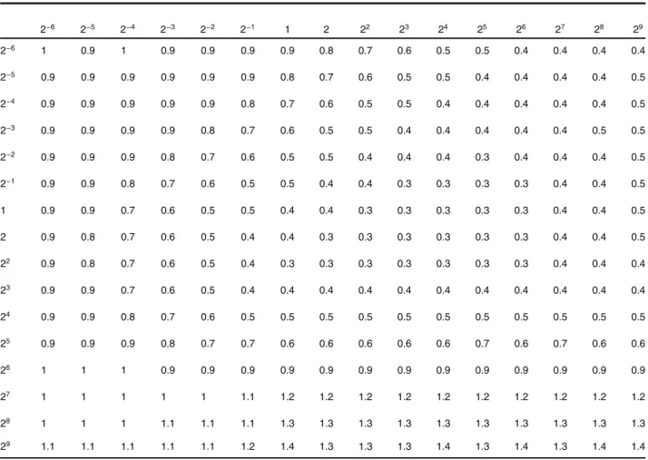
On the contrary, Tables3and4show that there are some pairs of values for parameters γ and C giving both a low Ierr
score and a fast classification, for example, γ¼ 4 and C ¼ 4, γ¼ 4 and C ¼ 8, γ ¼ 8, C ¼ 8, etc.
We explain the difference between the two classifiers by the fact that SVM uses the whole training data, whereas RF trains each decision tree with a subset of the training data. In interactive segmentation problems, the low number of training data (especially when dealing with superpixels, Table 1 Execution time (in a tenth of a second) of RF classifier, achieved on a subset of the ground truth of Santner et al.26 The first row gives the percentage of training data per tree, the first column gives the number of trees.
10 20 30 40 50 60 70 80 90 100 100 0.8 1.6 2.6 3.3 4.1 4.9 5.7 6.6 7.4 8 200 1.1 2.1 3.2 4.4 5.5 6.4 7.5 8.6 9.8 10.5 300 1.3 2.5 3.8 5.1 6.5 7.7 9 10.3 11.8 12.7 400 1.4 2.9 4.4 6 7.3 8.8 10.8 11.9 13.5 15.2 500 1.6 3.2 5 6.6 8.3 10 11.6 13.4 15.4 16.9 600 1.7 3.5 5.6 7.5 9.3 11.1 12.9 14.8 17 18.5 700 1.9 3.8 6.5 8.1 10 11.9 14.1 16.2 18 19.6 800 2.1 4.2 6.8 8.8 10.8 12.9 15.9 17.9 19.1 21.3 900 2.2 4.5 7.3 9.4 11.7 14.1 17 19.1 20.5 22.9 1000 2.4 5 7.6 9.9 12.8 14.9 18 20.6 22 24.6
Table 2 Error rate Ierr(%) of RF classifier, achieved on a subset of
the ground truth of Santner et al.26The first row gives the percentage of training data per tree, the first column gives the number of trees.
10 20 30 40 50 60 70 80 90 100 100 13 13 13 13 13 13 13 13 13 13 200 10 9 9 10 9 10 10 9 9 9 300 8 8 8 8 8 8 8 8 8 8 400 7 7 7 7 7 7 7 7 7 7 500 6 6 6 6 6 6 6 6 6 6 600 6 6 6 6 6 6 6 6 6 6 700 5 5 5 5 5 5 5 5 5 5 800 5 5 5 5 5 5 5 5 5 5 900 5 5 5 5 5 5 5 5 5 5 1000 5 5 5 5 5 5 5 5 5 5
less numerous than pixels) makes the learning task difficult for a classifier such as RF.
3.4 Parameter Values
In all our tests, following the recommendation of Achanta et al.,45 we used the SLIC oversegmentation algorithm with a compactness parameter equal to 10. In SαF, we group pixels into about 3000 superpixels. For the SVM, γparameter was equal to 4 and C parameter was equal to 4. On all experimental datasets, these values provide satisfac-tory results, but are not critical.
4 Evaluation of SαF
4.1 State-of-the-Art Benchmarks
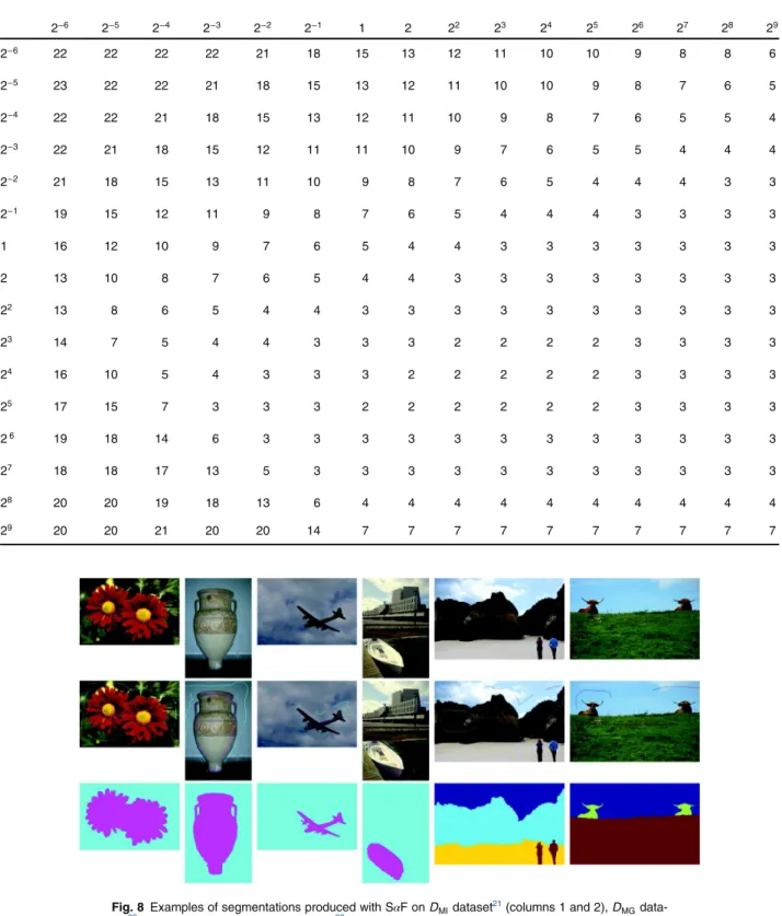
We compared SαF to results achieved by the height of state-of-the-art methods: three region-based interactive binarization methods (IGC,16 SIOX,17 and BPT25), one boundary-based interactive binarization method (CPP),21and four multiclass methods (SRG,15IMS,26RIMSAED,28and RIIS32). Figure 8 shows examples of segmentations pro-duced by SαF on images of state-of-the-art benchmarks. 4.1.1 Method of Milles et al.
We compare SαF to the most recent boundary-based inter-active segmentation method: CPP. This algorithm has
been evaluated by Mille et al.21on a subset of 10 images, extracted from the dataset DMI provided by Microsoft.56
The accuracy of the obtained segmentations is quantified using the AOmeasure of McGuinness and Oconnor29
EQ-TARGET;temp:intralink-;e009;326;313AOðR; GÞ ¼ 100
jGO∩ ROj
jGO∪ ROj
; (9)
where ROis the set of pixels labeled as object by the
algo-rithm, GOis the set of pixels labeled as object in the ground
truth, and jSj is the cardinality of a set S. A high value of AO indicates that the resulting regions and the regions in
the ground truth are similar.
Milles et al.21used automatically generated seeds: using the ground truth, the boundary of the object is extracted and split into N segments of equal length. For each segment, a seed is randomly selected. For a same image, Milles et al.21 computed 20 different sets of seeds. Table5shows the aver-age, the standard deviation, and the maximum value of AO
scores achieved by CPP method.
Table 6shows the performances of SαF with the same images using manually given seeds. During 2 min, the user is allowed to update seeds, improving the segmentation. The average percentage of pixels labeled as seeds by the user is equal to 0.56%.
Unfortunately, results presented in Tables5and6are not comparable. The seeds used for the evaluation of CPP are
2−6 2−5 2−4 2−3 2−2 2−1 1 2 22 23 24 25 26 27 28 29 2−6 1 0.9 1 0.9 0.9 0.9 0.9 0.8 0.7 0.6 0.5 0.5 0.4 0.4 0.4 0.4 2−5 0.9 0.9 0.9 0.9 0.9 0.9 0.8 0.7 0.6 0.5 0.5 0.4 0.4 0.4 0.4 0.5 2−4 0.9 0.9 0.9 0.9 0.9 0.8 0.7 0.6 0.5 0.5 0.4 0.4 0.4 0.4 0.4 0.5 2−3 0.9 0.9 0.9 0.9 0.8 0.7 0.6 0.5 0.5 0.4 0.4 0.4 0.4 0.4 0.5 0.5 2−2 0.9 0.9 0.9 0.8 0.7 0.6 0.5 0.5 0.4 0.4 0.4 0.3 0.4 0.4 0.4 0.5 2−1 0.9 0.9 0.8 0.7 0.6 0.5 0.5 0.4 0.4 0.3 0.3 0.3 0.3 0.4 0.4 0.5 1 0.9 0.9 0.7 0.6 0.5 0.5 0.4 0.4 0.3 0.3 0.3 0.3 0.3 0.4 0.4 0.5 2 0.9 0.8 0.7 0.6 0.5 0.4 0.4 0.3 0.3 0.3 0.3 0.3 0.3 0.4 0.4 0.5 22 0.9 0.8 0.7 0.6 0.5 0.4 0.3 0.3 0.3 0.3 0.3 0.3 0.3 0.4 0.4 0.4 23 0.9 0.9 0.7 0.6 0.5 0.4 0.4 0.4 0.4 0.4 0.4 0.4 0.4 0.4 0.4 0.4 24 0.9 0.9 0.8 0.7 0.6 0.5 0.5 0.5 0.5 0.5 0.5 0.5 0.5 0.5 0.5 0.5 25 0.9 0.9 0.9 0.8 0.7 0.7 0.6 0.6 0.6 0.6 0.6 0.7 0.6 0.7 0.6 0.6 26 1 1 1 0.9 0.9 0.9 0.9 0.9 0.9 0.9 0.9 0.9 0.9 0.9 0.9 0.9 27 1 1 1 1 1 1.1 1.2 1.2 1.2 1.2 1.2 1.2 1.2 1.2 1.2 1.2 28 1 1 1 1.1 1.1 1.1 1.3 1.3 1.3 1.3 1.3 1.3 1.3 1.3 1.3 1.3 29 1.1 1.1 1.1 1.1 1.1 1.2 1.4 1.3 1.3 1.3 1.4 1.3 1.4 1.3 1.4 1.4
Table 3 Execution time (in a tenth of a second) of SVM classifier, achieved on a subset of the ground truth of Santner et al.26 The first row gives the value of C parameter, the first column gives the value of parameter γ.
created using the ground truth and are more accurately located than seeds manually given by a user. In addition, seeds used for the evaluation of SαF are updated by the user.
With less than three iterations, SαF is able to achieve very satisfactory results on these datasets. In addition, SαF execution time does not depend on the number of seeds. Section 4.3 shows that this execution time is related to
2−6 2−5 2−4 2−3 2−2 2−1 1 2 22 23 24 25 26 27 28 29 2−6 22 22 22 22 21 18 15 13 12 11 10 10 9 8 8 6 2−5 23 22 22 21 18 15 13 12 11 10 10 9 8 7 6 5 2−4 22 22 21 18 15 13 12 11 10 9 8 7 6 5 5 4 2−3 22 21 18 15 12 11 11 10 9 7 6 5 5 4 4 4 2−2 21 18 15 13 11 10 9 8 7 6 5 4 4 4 3 3 2−1 19 15 12 11 9 8 7 6 5 4 4 4 3 3 3 3 1 16 12 10 9 7 6 5 4 4 3 3 3 3 3 3 3 2 13 10 8 7 6 5 4 4 3 3 3 3 3 3 3 3 22 13 8 6 5 4 4 3 3 3 3 3 3 3 3 3 3 23 14 7 5 4 4 3 3 3 2 2 2 2 3 3 3 3 24 16 10 5 4 3 3 3 2 2 2 2 2 3 3 3 3 25 17 15 7 3 3 3 2 2 2 2 2 2 3 3 3 3 26 19 18 14 6 3 3 3 3 3 3 3 3 3 3 3 3 27 18 18 17 13 5 3 3 3 3 3 3 3 3 3 3 3 28 20 20 19 18 13 6 4 4 4 4 4 4 4 4 4 4 29 20 20 21 20 20 14 7 7 7 7 7 7 7 7 7 7
Fig. 8Examples of segmentations produced with SαF on DMIdataset21(columns 1 and 2), DMG
data-set29(columns 3 and 4) and D
SAdataset26(columns 5 and 6). The first row shows the original image,
the second row the given seeds, and the third row the result.
Table 4 Error rate Ierr (%) of SVM classifier, achieved on a subset of the ground truth of Santner et al.26 The first row gives the value of C
the number of pixels during the initialization stage and to the number of superpixels during the segmentation stages. The initialization stage can be done once, while the user is selecting the first seeds. So, only the execution time of the segmentation is perceived by the user. On the contrary, CPP execution time depends both on the image size and on the number of seeds. The average execution time for SαF is equal to 0.4 s for the initialization stage and to 0.2 s for each segmentation stage. The execution time of CPP varies between 3 and 17 s using similar hardware.
4.1.2 Methods evaluated by McGuinness et al. The methods SRG, IGC, SIOX, and BPT have been evalu-ated by McGuinness et al.29on the dataset DMGprovided by
the authors,56using boundary (A
B) and object (AO) accuracy
measures.29Given a segmentation result R and a ground truth G, the boundary accuracy measure is given by
EQ-TARGET;temp:intralink-;e010;326;575ABðR; GÞ ¼ 100 P xmin½ ˜BGðxÞ; ˜BR ðxÞ-P x max½ ˜BGðxÞ; ˜BR ðxÞ-; (10)
where BG and BR are the internal border pixels for ground
truth and algorithm segmentation result, respectively, and ˜BG
and ˜BR are these same sets extended using fuzzy-set theory
as described in the paper of McGuinness et al.29A high value of AB score indicates that boundaries in the segmentation
result follow boundaries in the ground truth.
For each method, seeds are manually given by a user. The user has 2 min to update these seeds and achieve a segmen-tation as accurate as possible.
Table7shows that SαF outperforms these four methods with a 5% increase on AB, a 3% increase on AO, and a similar
execution time.
4.1.3 Method of Jian et al.
We cannot make a rigorous comparison between SαF and a recent interactive binarization method based on an ACP, proposed by Jian and Jung31 Indeed, this paper does not contain sufficient information about the dataset used, which is an extended version of the one created by McGuinness and Oconnor.29 We simply notice that SαF results on McGuinness et al. dataset29are superior to ACP scores reported by the authors, with a 1% increase. SαF exe-cution times are slightly superior, but this drawback must be balanced by the possibility to compute the initialization stage while the user gives the seeds, to obtain a perceived SαF execution time less than or equal to ACP.
4.1.4 Methods of Santner et al. and Müller et al. IMS and RIMSAED have been evaluated by Santner et al.26 using the dataset DSA55 provided by the authors and the
DICE measure, suggested by Dice and defined in their paper. This measure is an adaptation of AO for multiclass
problems EQ-TARGET;temp:intralink-;e011;326;147DICEðR; GÞ ¼ 100 XK i¼1 2jRi∩ Gij jRi∪ Gij ; (11)
where K is the number of classes, Riis the set of pixels of the
i’th class in the resulting segmentation, and Giis the set of
pixels of the i’th class in the ground truth. Table 5 Performances achieved by CPP, reported from the paper of
Milles et al.21
Image CPP avg CPP std CPP max
Banana1 60.4 0.20 89.1 Banana2 47.3 0.25 88.3 Banana3 62.5 0.15 86.6 Ceramic 85.6 0.03 89.8 Doll 80.8 0.04 87.7 Flower 88.1 0.29 98.2 Mushroom 61.3 0.17 91.1 Music 97.8 0.01 98.6 Sheep 77.0 0.18 90.2 Teddy 74.9 0.17 96.7 All 73.5 0.23 91.4
Table 6 Performances achieved by SαF.
Image SαF Banana1 97.1 Banana2 96.4 Banana3 97.9 Ceramic 97.5 Doll 98.9 Flower 98.6 Mushroom 97 Music 98.9 Sheep 96.2 Teddy 95.8 All 97.2
Table 7 Evaluation of SαF with McGuinness et al. protocol and com-parison with IGC, SIOX, BTP, and SRG methods.29
IGC SIOX BTP SRG SαF
AO 92 85 92 88 95
Both Santner et al.26and Müller et al.28used the same seeds, given by the user during the creation of the ground truth. These seeds are not updated to improve the segmen-tation result.
With these seeds, the overall performance of SαF is not satisfactory, with an average DICE score of 83. The values vary between 40 and 99 and the standard deviation is around 14, indicating a high dispersion. A detailed analysis of the score distribution shows that the dataset can be divided into three groups: 32% of the images give a very good DICE score (more than 93), 35% a good DICE score (between 80 and 93), and 33% a bad DICE score (less than 80). This latter category of images explains the weak average performance of SαF.
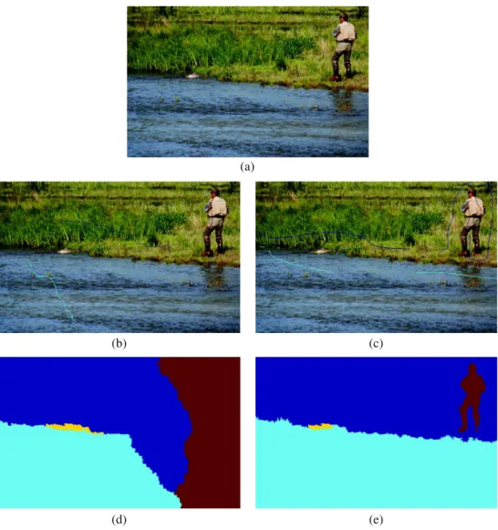
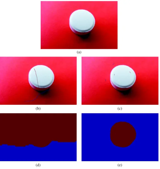
For these images, the provided seeds are not suitable to SαF. Because SαF uses location information, it obtains unsatisfactory results when seeds are given too far from the object boundaries. Examples of such unsuitable locations are given in Figs.9and10. For some images, seeds need to be located near the boundaries and more numerous (Fig.9).
For others, modifying their locations is enough for SαF to get good results (Fig. 10).
To produce accurate results, SαF needs an instruction to be given to the user: “give the initial seeds near the object boundaries.” In the case of DSAdataset, a maximum distance
around 30 pixels is quite enough. As explained in Sec.4.4, this is a small price to pay for a method showing an easily predictable behavior.
For each image, we made an additional test taking into account the instruction and allowing the user to modify the seeds in order to improve the segmentation result. We calculated the DICE score obtained with two sets of seeds: the set of initial seeds given before the first segmentation and the set of final seeds selected when the user is satisfied with the result. The average number of updates between the first segmentation and the final result is equal to 3. SαF produced accurate results with an average DICE score of 97 for the set of initial seeds and of 98 for the set of final seeds. The average execution time of SαF was only 1.2 s against 2 s for IMS and for RIMSAED. In addition, these execution (a)
(b) (c)
(d) (e)
Fig. 9Examples where seeds of Santner et al.26are inadequate in location and number for SαF to accu-rately segment the image. (a) Image 0011, (b) seeds of Santner et al., (c) seeds given by asking the user to select them near the object boundaries, (d) result with seeds of Santner et al., and (e) Result with seeds near the object boundaries.
times, on the contrary for IMS and RIMSAED, are achieved without any specific optimization. In particular, SαF does not require a GPU implementation.
4.1.5 Method of Oh et al.
RIIS has been evaluated on DMIand DSAdatasets, both with
DICE measure, with manually given seeds. In the same con-ditions, SαF outperforms RIIS in terms of accuracy, with a 5% increase on DMIdataset and an 8% increase on DSA
data-set (Table8). The method SαF is also much more efficient with an execution time of about 1 s on a simple desktop com-puter, whereas RIIS running time is greater than 40 s.
4.2 Benefit of the Regularization Term
To analyze the benefit of the regularization term, we design more simple versions of SαF minimizing
EQ-TARGET;temp:intralink-;e012;326;270ESCISðcjIÞ ¼
YN
i¼1
Idataðx
i; ciÞ: (12)
The minimization of ESCISis easily achieved by simply
keeping the classification produced by the SVM. So, we name this algorithm SCIS for superpixel classification-based interactive segmentation. We made tests on DMG, DMI,29and
DSAdataset.26Table9gives the percentage of pixels used as
seeds (Pr), execution time (s) for the initialization step (Tinit),
and segmentation time (s) for the segmentation step, which are required for both SCIS and SαF achieve similar accuracy. In other words, AOand ABscores on DMGdataset,29AOscore
on DMI dataset,21 and DICE score on DSA dataset26 are
similar.
These results show that the introduction of a regularization term in SαF reduces the required number of pixels labeled as seeds of about 1%. Concretely, SCIS uses more than 200,000 supplementary seeds. In addition, these seeds cannot be (a)
(b) (c)
(d) (e)
Fig. 10Examples where seeds of Santner et al.26are inadequate in location for SαF to accurately seg-ment the image. (a) Image 0217, (b) seeds of Santner et al., (c) seeds given by asking the user to select them near the object boundaries, (d) Result with seeds of Santner et al., and (e) Result with seeds near the object boundaries.
obtained by giving a simple instruction. Figure 11 shows an example of differences between SCIS and SαF seeds. Execution time is not significantly increased by introducing the regularization term. The initialization stage is not impacted and the segmentation stage remains about 1 s.
4.3 Scalability
We also investigate the ability of SαF to segment images of various sizes, especially images with several million pixels. As none of the previous benchmarks provides a dataset with such images, we selected 50 images from HSID and adapted them to evaluate multiclass interactive segmentation meth-ods. We created four datasets, by rescaling these images and the ground truth: the first with big images (2,161,800 pix-els), the second with medium images (1,216,350 pixpix-els), the third with small images (684,788 pixels), and the last with tiny images (167,000 pixels).
For each dataset, we compute the mean, the standard deviation, the minimum value and the maximum value of the execution time for the initialization stage (Table 10),
the execution time for the segmentation stage (Table 11) and the DICE measure (Table12).
The low standard deviation and the small difference between maximum and minimum values shows that the quality of SαF results and the time required are not strongly altered by the number of classes. The most interesting con-clusion on this experimentation is the gap between the exe-cution time for the initialization stage and the exeexe-cution time for the segmentation stage. As initialization must be done only once, this stage has little impact on SαF responsiveness. In fact, with an implementation performing this stage while the user gives seeds, SαF can become an interactive time application, computing the segmentation stage in less than 1 s, even for images with millions of pixels. In addition, because the superpixel number is always around 3000, the execution time for the segmentation stage is stable, even if the image size is significantly increased. The DICE score shows that this “compression” of the image is sufficient to ensure accurate results, no matter the image size.
Table 8 Comparison between RIIS and SαF on the DMIand the DSA
datasets, with the DICE measure (%).
RIIS SαF
DMI,21DICE 93 98
DSA,26DICE 90 98
Table 9 Comparison of the required percentage of pixels labeled as seeds (Pr), execution time in seconds for the initialization step (Tinit) and
segmentation time in seconds for the segmentation step (Tseg) for both SCIS and SαF. The three scores are obtained for segmentations of similar
accuracy.
Bench.
DMG29 DMI21 DSA26
SCIS SαF SCIS SαF SCIS SαF
Pr (%) 2.08 . 0.49 1.26 . 0.69 2.08 . 0.49 0.74 . 0.36 1.42 . 0.42 0.89 . 0.43 TinitðsÞ 0.4 . 0.01 0.41 . 0.01 0.6 . 0.18 0.61 . 0.19 0.64 . 0.02 0.66 . 0.02 TsegðsÞ 0.06 . 0.03 0.68 . 0.04 0.04 . 0.02 0.27 . 0.02 0.06 . 0.04 0.51 . 0.28
(a) (b)
Fig. 11 Comparison between (a) SCIS and (b) SαF seeds.
Table 10 SαF initialization stage execution time in seconds.
Size Mean . std Min Max
Tiny 0.47 . 0.08 0.42 1.03
Small 1.79 . 0.06 1.71 1.98
Medium 3.25 . 0.12 3.06 3.64
4.4 Usability
4.4.1 Time required to segment an image
A fully manual segmentation of an image is a time-consum-ing task. To create the reference segmentations of HSID, we spent around 1 h per image to achieve a level of accuracy high enough to meet the requirements of a ground truth
data. However, we are comfortable with graphic tablets. Beginners need more time to get an accurate segmentation. Using SαF significantly facilitates and accelerates the seg-mentation process. The overall time to segment an image— including the selection of initial seeds, the corrections of seeds and the execution time of each use of SαF—is related: • to the number of classes: several classes require more seeds and to often change the color of the brush-like tool used to select them;
• to the image complexity: if an object contains a lot of small and scattered details, selection of seeds is more difficult.
With McGuinness et al.,29in the worst case, the overall time is 2 min. In the best case, only a few seconds are required to segment an image. With Santner et al.,26 in the worst case, this duration is around 5 min. In the best case, only a few seconds are required to segment an image. The selection of the initial seeds is the more time-consuming task. The computation time of each run of the segmentation stage of SαF is lower than 1 s. The correction of seeds takes only a few seconds.
Table13shows three examples of time needed for fully manually segmenting an image versus using SαF. The first image (Fig. 12) is a small image of the McGuinness et al. dataset,29 whereas the last two images (Figs. 13 and 14) come from the HSID dataset. The overall segmentation time using SαF is detailed into the last four columns of this table. On these images, using SαF is 6 to 11 times faster than a fully manual segmentation.
Table 11 SαF segmentation stage execution time in seconds.
Size Mean . std Min Max
Tiny 0.49 . 0.27 0.23 1.69
Small 0.46 . 0.28 0.21 1.64
Medium 0.46 . 0.28 0.21 1.68
Big 0.41 . 0.22 0.2 1.2
Table 12 SαF DICE score.
Size Mean . std Min (%) Max (%)
Tiny 98%. 4.72 66 100
Small 99%. 1.03 95 100
Medium 99%. 0.99 95 100
Big 99%. 1.12 95 100
Table 13 Examples of time needed for a user to perform a fully manual segmentation of an image versus using SαF (s).
Image Fully manual
Using SαF
Overall time Initial seed selection Seed corrections Initialization stage Segmentation stage
Fig.12 216 34 27 5 0.5 1.5
Fig.13 634 37.5 25 6 5.5 1
Fig.14 893 76.5 62 8 5.5 1
Fig. 12SαF seed evolution example for a binarization problem. Only two updates of seeds are required to achieve an accurate result.
In the case of Fig.12, where a church must be extracted and where the foreground is clearly separate from the back-ground, only a few seeds are necessary. The user who seg-mented this image was familiar with SαF: drawing some strokes to obtain the first segmentation result took only a few seconds. Additional tests show us that less experienced users need more time (several tens of seconds) for the first image because they select more seeds, following more scrupulously the object boundaries. Fortunately, they learn quickly how to reduce the number of seeds. The correction of errors in the result given by SαF by adding or removing seeds is straightforward: for both novice and expert users, each correction takes less than 1 s.
4.4.2 Predictability
The user evaluation results of the McGuinness et al. review29 highlight the necessity for an interactive segmentation method to not only provide a fast and accurate segmentation, but also to have a predictable behavior.
Figures12–14show examples of segmentations achieved with SαF for images taken from datasets used in Secs.4.1
and 4.3. The analysis of the given seeds shows that the behavior of SαF is easily predictable: by putting seeds near the objects borders, the majority of the image is cor-rectly segmented. In the majority of the cases, the remaining errors are quickly corrected by adding seeds over them. If some errors are due to seeds put on the wrong object, these seeds can be removed. This good predictability is directly related to the choice of the superpixel features: as color and location are extremely intuitive concepts, the behavior of SαF is consistent with the user expectation.
Moreover, for the images of Figs.12–14, a maximum of two updates of the seeds allow achieving a correct segmen-tation. Except for particularly difficult situations with, for example, shadows or a poor contrast between objects, the required number of iterations varies from 2 to 4. If seeds are correctly positioned with respect the object boundaries, only small errors have to be corrected and the accuracy of the segmentation at each iteration is not strongly improved. For example, on the dataset of Santner et al.,26between the initial and the final segmentations, the average DICE score has improved from about 97 to 98. This fast convergence and Fig. 13SαF seed evolution example for a problem with three classes. Only one update of seeds is
required to achieve an accurate result.
Fig. 14SαF seed evolution example for a problem with four classes. Only two updates of seeds are required to achieve an accurate result.
the fact that only some strokes are required to segment an image make us confident about the user acceptance of SαF as a tool for multiple object selection.
However, when first seeds are not given near the boun-dary, SαF can produce segments with significant errors. Notably, if the seeds are given only on a small part of the image, superpixels used as training data can be insufficient to find the right support vector during SVM training. An example is given in Fig. 15. Fortunately, these errors are easily avoided by asking the user to give seeds near the boundaries.
5 Applications
5.1 Semantic Segmentation for Landscape Observatories
Since 2005, the European Landscape Convention of the Council of Europe57promotes the protection and manage-ment of European landscapes. In this context, landscape observatories58–60respond to the need to study the landscape
and build awareness of society to their conservation. They are based on digital photograph datasets, containing for sev-eral interesting spots a chronological series of photographies, taken regularly (for example, every month or every year).
The algorithm SαF has been implemented in an Android application allowing to update the images of a landscape observatory and to segment them into labeled regions, related to landscape semantic elements (building, grass, road, etc.). The application locates the nearest observatory spot and downloads a previous photograph of the spot to easily re-photograph it. Then, it uses SαF to produce semantic seg-mentation of the photograph, which allows a quick automatic comparison of images of the same spot to detect interesting changes. The complete framework has been presented during the 2017 French Conference on Multimedia, Geomatics,
Teaching, and Learning61and will be used very soon with school students in life and agronomy sciences and technol-ogies and landscape design.
5.2 Photograph Enhancement
Figure16shows an example of SαF usage to enhance a pho-tograph using Gimp. Thanks to SαF, three different image regions are selected, corresponding to the sky, the building, and the water. Notice that the original image is especially difficult with a poor contrast between the water and the buildings, dull colors, and thin elements. Then, we applied to each region a specific operator to enhance it and modified the color channels of the sky to create a sunset feeling; we increased the contrast and the color saturation of the build-ings and made the water darker with golden light reflections. Each local modification allows a more visually pleasant global image.
6 Conclusions
In this paper, we proposed an interactive multiclass segmen-tation method, SαF. This algorithm is based on the modeling of the interactive segmentation problem as a factor graph, where variables are superpixels and factors allow to mini-mize both a data term and a regularization term. By compar-ing SαF with the state-of-the-art algorithms on current benchmarks, we show that it is a very competitive algorithm. We also provide extended tests, allowing to better understand the influence of each component of the proposed method. In particular, we made available a dataset for oversegmentation methods evaluation, providing results missed by the previous reviews about superpixel algorithms. In addition, we made available three datasets to check scalability of interactive segmentation methods and show that SαF successfully seg-ments them.
(a) (b)
Fig. 15SαF failing to produce an accurate segmentation when user gives wrong seeds. (a) SαF seeds and (b) segmentation result.
Fig. 16Usage of SαF for photo enhancement. From the left to the right: original image, seeds, segmen-tation result, and enhanced photograph.
The performance achieved by SαF on the six tested data-sets shows the ability of superpixels to provide an efficient compression of the image. The execution time of SαF high-lights their relevance to design competitive computer vision algorithms. Here, they are the key to provide a scalable method producing a result in interactive time.
We also described SαF usage in two different applica-tions: photograph enhancement and semantic segmentation. The source code of SαF, the three datasets used for the scalability evaluation, and the seeds are made available at Ref.56.
Acknowledgments
The work of Bérengère Mathieu was partially supported by LABX-0040-CIMI within the program ANR-11-IDEX-0002-02.
References
1. J. Long, E. Shelhamer, and T. Darrell, “Fully convolutional networks for semantic segmentation,” inIEEE Conf. on Computer Vision and Pattern Recognition, pp. 3431–3440 (2015).
2. A. Garcia-Garcia et al., “A review on deep learning techniques applied to semantic segmentation,” Comput. Res. Repository abs/1704.06857 (2017).
3. D. Fourure et al., “Multi-task, multi-domain learning: application to semantic segmentation and pose regression,” Neurocomputing 251, 68–80 (2017).
4. D. Lin et al., “ScribbleSup: scribble-supervised convolutional networks for semantic segmentation,” inIEEE Conf. on Computer Vision and Pattern Recognition, pp. 3159–3167 (2016).
5. N. Ben-Zadok, T. Riklin-Raviv, and N. Kiryati, “Interactive level set segmentation for image-guided therapy,” in IEEE Int. Symp. on Biomedical Imaging: From Nano to Macro, pp. 1079–1082 (2009). 6. D. Cremers et al., “A probabilistic level set formulation for interactive
organ segmentation,”Proc. SPIE6512, 65120V (2007).
7. A. X. Falcão, J. K. Udupa, and F. K. Miyazawa, “An ultra-fast user-steered image segmentation paradigm: live wire on the fly,” IEEE Trans. Med. Imaging19(1), 55–62 (2000).
8. Y. Gao et al., “A 3D interactive multi-object segmentation tool using local robust statistics driven active contours,” Med. Image Anal.
16(6), 1216–1227 (2012).
9. Y. Tong et al., “Interactive iterative relative fuzzy connectedness lung segmentation on thoracic 4D dynamic MR images,”Proc. SPIE10137, 1013723 (2017).
10. J. Egger et al., “US-cut: interactive algorithm for rapid detection and segmentation of liver tumors in ultrasound acquisitions,”Proc. SPIE
9790, 97901C (2016).
11. H.-E. Gueziri, M. J. McGuffin, and C. Laporte, “A generalized graph reduction framework for interactive segmentation of large images,”
Comput. Vision Image Understanding150, 44–57 (2016).
12. T. Suzuki et al., “Interactive segmentation of pancreases from abdomi-nal CT images by use of the graph cut technique with probabilistic atlases,” in Int. Conf. on Innovation in Medicine and Healthcare, pp. 575–584, Springer (2015).
13. P. Karasev et al., “Interactive medical image segmentation using PDE control of active contours,”IEEE Trans. Med. Imaging32, 2127–2139 (2013).
14. J. Petersena et al., “Effective user guidance in online interactive seman-tic segmentation,”Proc. SPIE10134, 101341V (2017).
15. R. Adams and L. Bischof, “Seeded region growing,” IEEE Trans. Pattern Anal. Mach. Intell.16(6), 641–647 (1994).
16. Y. Boykov and M.-P. Jolly, “Interactive graph cuts for optimal boundary and region segmentation of objects in ND images,” inIEEE Int. Conf. on Computer Vision, Vol. 1, pp. 105–112 (2001).
17. G. Friedland, K. Jantz, and R. Rojas, “SIOX: simple interactive object extraction in still images,” inIEEE Int. Symp. on Multimedia(2005). 18. L. Grady, “Random walks for image segmentation,” IEEE Trans.
Pattern Anal. Mach. Intell.28(11), 1768–1783 (2006).
19. V. Gulshan et al., “Geodesic star convexity for interactive image seg-mentation,” inIEEE Computer Society Conf. on Computer Vision and Pattern Recognition, pp. 3129–3136 (2010).
20. Y. Li et al., “Lazy snapping,”ACM Trans. Graphics23(3), 303–308 (2004).
21. J. Mille, S. Bougleux, and L. D. Cohen, “Combination of piecewise-geodesic paths for interactive segmentation,”Int. J. Comput. Vision
112(1), 1–22 (2015).
22. P. A. Miranda, A. X. Falcao, and T. V. Spina, “Riverbed: a novel user-steered image segmentation method based on optimum boundary tracking,”IEEE Trans. Image Process.21(6), 3042–3052 (2012).
23. E. N. Mortensen and W. A. Barrett, “Interactive segmentation with intelligent scissors,”Graphical Models Image Process.60(5), 349–384 (1998).
24. J. Ning et al., “Interactive image segmentation by maximal similarity based region merging,”Pattern Recognit.43(2), 445–456 (2010). 25. P. Salembier and L. Garrido, “Binary partition tree as an efficient
representation for image processing, segmentation, and information retrieval,”IEEE Trans. Image Process.9(4), 561–576 (2000). 26. J. Santner, T. Pock, and H. Bischof, “Interactive multi-label
segmenta-tion,” in Asian Conf. on Computer Vision, pp. 397–410 (2010). 27. A. Blake et al., “Interactive image segmentation using an adaptive
GMMRF model,” in European Conf. on Computer Vision, pp. 428– 441 (2004).
28. S. Müller et al., “Robust interactive multi-label segmentation with an advanced edge detector,” in German Conf. on Pattern Recognition, pp. 117–128 (2016).
29. K. McGuinness and N. E. Oconnor, “A comparative evaluation of interactive segmentation algorithms,”Pattern Recognit.43(2), 434–444 (2010).
30. Y. Rubner, C. Tomasi, and L. J. Guibas, “The earth mover’s distance as a metric for image retrieval,” Int. J. Comput. Vision40(2), 99–121 (2000).
31. M. Jian and C. Jung, “Interactive image segmentation using adaptive constraint propagation,”IEEE Trans. Image Process.25(3), 1301–1311 (2016).
32. C. Oh, B. Ham, and K. Sohn, “Robust interactive image segmentation using structure-aware labeling,”Expert Syst. Appl.79, 90–100 (2017). 33. P. Dollár and C. L. Zitnick, “Fast edge detection using structured forests,”IEEE Trans. Pattern Anal. Mach. Intell.37(8), 1558–1570 (2015).
34. C. Nieuwenhuis and D. Cremers, “Spatially varying color distributions for interactive multilabel segmentation,” IEEE Trans. Pattern Anal. Mach. Intell.35(5), 1234–1247 (2013).
35. D. Krishnan, R. Fattal, and R. Szeliski, “Efficient preconditioning of Laplacian matrices for computer graphics,” ACM Trans. Graphics
32(4), 142 (2013).
36. J. Kappes et al., “A comparative study of modern inference techniques for discrete energy minimization problems,” in IEEE Conf. on Computer Vision and Pattern Recognition, pp. 1328–1335 (2013). 37. D. Stutz, “Superpixel segmentation: an evaluation,” in German Conf. on
Pattern Recognition, pp. 555–562 (2015).
38. D. Koller and N. Friedman, Probabilistic Graphical Models: Principles and Techniques, MIT Press, Cambridge (2009).
39. T.-F. Wu, C.-J. Lin, and R. C. Weng, “Probability estimates for multi-class classification by pairwise coupling,” J. Mach. Learn. Res. 5, 975–1005 (2004).
40. Y. Boykov, O. Veksler, and R. Zabih, “Fast approximate energy min-imization via graph cuts,”IEEE Trans. Pattern Anal. Mach. Intell.
23(11), 1222–1239 (2001).
41. A. Fix et al., “A graph cut algorithm for higher-order Markov random fields,” inIEEE Int. Conf. on Computer Vision, pp. 1020–1027 (2011). 42. P. F. Felzenszwalb and D. P. Huttenlocher, “Efficient graph-based image
segmentation,”Int. J. Comput. Vision59(2), 167–181 (2004). 43. A. Vedaldi and S. Soatto, “Quick shift and kernel methods for
mode seeking,” in European Conf. on Computer Vision, pp. 705–718 (2008).
44. M.-Y. Liu et al., “Entropy rate superpixel segmentation,” inIEEE Conf. on Computer Vision and Pattern Recognition, pp. 2097–2104 (2011). 45. R. Achanta et al., “SLIC superpixels compared to state-of-the-art superpixel methods,”IEEE Trans. Pattern Anal. Mach. Intell.34(11), 2274–2282 (2012).
46. C. Conrad, M. Mertz, and R. Mester, “Contour-relaxed superpixels,” in Int. Workshop on Energy Minimization Methods in Computer Vision and Pattern Recognition, pp. 280–293 (2013).
47. A. Rubio et al., “BASS: boundary-aware superpixel segmentation,” in
Int. Conf. on Pattern Recognition(2016).
48. V. Machairas et al., “Waterpixels,”IEEE Trans. Image Process.24(11), 3707–3716 (2015).
49. B. Mathieu, A. Crouzil, and J. B. Puel, “Heterogeneous size image data-set,”image.ensfea.fr/hsid/(2017).
50. B. Mathieu, A. Crouzil, and J. B. Puel, “Oversegmentation methods: a new evaluation,” in Iberian Conf. on Pattern Recognition and Image Analysis(2017).
51. S. Gould et al., “Multi-class segmentation with relative location prior,”
Int. J. Comput. Vision80(3), 300–316 (2008).
52. O. Barkan et al., “Fast high dimensional vector multiplication face recognition,” inIEEE Int. Conf. on Computer Vision, pp. 1960–1967 (2013).
53. S. Bochkanov, “ALGLIB®
–numerical analysis library,”www.alglib.net (1999).
54. C. C. Chang and C. J. Lin, “LIBSVM: a library for support vector machines,” ACM Transactions on Intelligent Systems and Technology (TIST) 2(3), 1–27http://www.csie.ntu.edu.tw/~cjlin/libsvm(2011). 55. J. Santner, “Interactive segmentation (IcgBench) dataset,”gpu4vision.