Official URL
DOI :
https://doi.org/10.23919/EUSIPCO.2019.8903037
Any correspondence concerning this service should be sent
to the repository administrator:
[email protected]
This is an author’s version published in:
http://oatao.univ-toulouse.fr/24982
Open Archive Toulouse Archive Ouverte
OATAO is an open access repository that collects the work of Toulouse
researchers and makes it freely available over the web where possible
To cite this version: Lagrange, Adrien and Fauvel, Mathieu and
May, Stéphane and Bioucas-Dias, José M. and Dobigeon, Nicolas
Matrix Cofactorization for Joint Unmixing and Classification of
Hyperspectral Images. (2019) In: 27th European Signal Processing
Conference (EUSIPCO 2019), 2 September 2019 - 6 September 2019
(A Coruna, Spain).
Abstract—This paper introduces a matrix cofactorization ap-proach to perform spectral unmixing and classification jointly. After formulating the unmixing and classification tasks as matrix factorization problems, a link is introduced between the two coding matrices, namely the abundance matrix and the feature matrix. This coupling term can be interpreted as a clustering term where the abundance vectors are clustered and the resulting attribution vectors are then used as feature vectors. The overall non-smooth, non-convex optimization problem is solved using a proximal alternating linearized minimization algorithm (PALM) ensuring convergence to a critical point. The quality of the obtained results is finally assessed by comparison to other conventional algorithms on semi-synthetic yet realistic dataset.
Index Terms—supervised learning, spectral unmixing, cofac-torization, hyperspectral images.
I. INTRODUCTION
Following the fast increase of available remote sensing images, many methods have been proposed to extract infor-mation from such specific data. In particular classification algorithms received a lot of attention from the scientific community. The emergence of state-of-the-art algorithms such as convolutional neural network [1] or random forest [2] have brought unprecedented good results. In the so-called supervised classification framework, these algorithms make it possible to infer, from a reduced number of examples provided by an expert, a classification rule. This rule is then used to attribute to unknown pixels a class among a predefined set of classes. Although very efficient, classification methods remain a limited analysis of the image since it only attributes a single class to each pixel when it is sometimes possible to extract more information. In the specific case of hyperspectral images (HSI), images capture a very rich signal since each pixel is a sampling of the reflectance spectrum of the corresponding area, typically in the visible and infrared spectral domains with hundreds of measurements. To fully exploit the available information, it is interesting to resort to alternative methods of interpretation such as representation learning methods, namely spectral unmixing in the case of HSI [3]. Spectral unmixing is
Part of this work has been supported Centre National d’ ´Etudes Spatiales (CNES), Occitanie Region, EU FP7 through the ERANETMED JC-WATER program, MapInvPlnt Project ANR-15-NMED-0002-02 and ANR-3IA Artifi-cial and Natural Intelligence Toulouse Institute (ANITI).
a physic-based model which assumes that a given pixel, i.e. a given measured spectrum, is the result of the combination of a reduced number of elementary spectra called endmembers, specific to a given material. The aim of unmixing methods is to infer the proportion of each material present in the pixel. The obtained abundance maps display the spatial distribution of the material in the observed scene.
Even if classification and spectral unmixing are two widely-used techniques, very few attempts have been made to com-bine them. Most of these works [4], [5] intend to improve classification results by using spectral unmixing to identify mixed pixels and then process specifically the identified mixed pixels. Instead of using the two methods sequentially, the method proposed in this paper introduces the idea of a joint unmixing and classification. This method is formulated as a cofactorization problem, which is known to produce valuable results in many application fields such as music source separa-tion [6], and image analysis [7]. The core concept is to express the two problems of interest, namely spectral unmixing and classification, as factorization problems and then to introduce a coupling term to intertwine the two estimations. Similarly to [8], the coupling term is defined as a clustering term where the abundance vectors provided by the unmixing step are clustered and the resulting attribution vectors are then used as feature vectors for the classification. The overall optimization problem is non-convex non-smooth. Such problems are known to be challenging to solve but, building on recent advances in optimization, the PALM algorithm proposed in [9] is used as an optimization scheme, thus guaranteeing convergence to a critical point of the objective function.
The rest of this paper is organized as follows. Section II defines the two factorization tasks and introduces the global cofactorization problem. Then, the method used to minimize the resulting criterion is presented in Section III. Finally, the method is tested and compared to other unmixing and classification methods in Section IV. Section V draws some conclusions and perspectives.
II. PROBLEM STATEMENT
As presented in Sections II-A and II-B, spectral unmixing and supervised classification are commonly expressed as fac-torization problems. We propose to derive a unified framework
Matrix
cofactorization for joint unmixing and
classification
of hyperspectral images
Adrien Lagrange⋆, Mathieu Fauvel†, St´ephane May‡, Jose´ M. Bioucas-Dias⋄ and Nicolas Dobigeon⋆ ⋆ IRIT/INP-ENSEEIHT, University of Toulouse, Toulouse, France
† Centre d’ ´Etudes Spatiales de la BIOsph`ere (CESBIO), INRA, Toulouse, France ‡ Centre National d’ ´Etudes Spatiales (CNES), DCT/SI/AP, Toulouse, France
⋄ Instituto de Telecomunicac¸ ˜oes, Instituto Superior Te´cnico, Universidade de Lisboa, 1049-001 Lisbon, Portugal
by considering a global cofactorization problem. It relies on a link between the two factorization problems in order to perform a joint estimation. In the proposed model, the link is made between the abundance matrix and the feature matrix. More precisely, the coupling term is expressed as a clustering term over the abundance vectors where the attribution vectors to the clusters are also the feature vectors of the classification as detailed in Section II-C.
A. Spectral unmixing
Each pixel of an HSI is a L-dimensional measurement of a reflectance spectrum. Physics models this spectrum as a combination of R elementary spectrum, gathered in the so-called endmember matrix M∈ RL×R, each characterizing a
specific material. The spectral unmixing task aims at retrieving the so-called abundance vectors ap ∈ RR, with R ≪ L,
from the spectrum yp ∈ RL of the pth pixel (p ∈ P where
P ! {1, . . . , P } is the set of pixel indexes). These abundance vectors describe the mixture contained in the pixel. Using the conventional linear mixture model, the spectral unmixing problem can be expressed as follow
min M,A 1 2&Y − MA& 2 F+ λa&A&1+ ıRR×P + (A) (1)
where matrix Y∈ RL×P gathers the P pixel spectra and A∈
RR×P the abundance vectors. In addition to the data fitting term, two penalization terms are considered in the proposed unmixing model. The term ıRR×P
+ (A) enforces a nonnegativity
constraint, ensuring an additive decomposition of the spectra. The second penalization λa&A&1 is a sparsity penalization
promoting the concept that only a few endmembers are active in a given pixel. In the following work, the choice has been made to discard the estimation of the endmember matrix for the sake of simplicity. The endmember matrix is assumed to be known or estimated beforehand.
B. Classification
In the context of supervised classification, a subset of pixels is available with their corresponding groundtruth. The index subset of labeled pixel is denoted hereafterL while the index subset of unlabeled pixel is U ( L ∩ U = ∅ and L ∪ U = P). Classification intends to assign one of the C classes to each pixel. In practice, classifying can be formulated as estimating a C × P matrix C whose columns correspond to unknown C-dimensional attribution vectors cp (p∈ U). Each vector is
made of0 except for ci,p= 1 when the pth pixel is assigned
the ith class. Numerous decision rules have been proposed to carry out classification. Most of them rely on the use of feature vectors zp ∈ RK (p ∈ P) associated with the P
pixels, gathered in the matrix Z ∈ RK×P. Considering a
linear classifier parametrized by the matrix Q ∈ RC×K, a
vector-wise nonlinear mapping φ(·), such as a sigmoid or a softmax operator, is then applied to the output of the classifier. Finally the classification rule can be expressed as the matrix factorization problem
min
Q,CU
Jc(C, φ(QZ)) + ıS|U |C (CU) (2)
where Jc(·, ·) is a cost function measuring the quality of the
estimated attribution vectors φ(Qzp) and and SC is the
C-dimensional probability simplex ensuring nonnegativity and sum-to-one constraints of the attribution vectors. In this work, the cost functionJc(·, ·) has been chosen as the cross-entropy,
defined in a multi-class problem as Jc(C, ˆC) = − ! p∈P dp ! i∈C
ci,plog (ˆci,p) (3)
with dp= " 1 |Li|, if p∈ Li, 1 |U |, if p∈ U, (4) whereLi is the subset of labeled pixels belonging to class i,
ˆ
cpis the estimated attribution vector and cp the true one. The
weighing coefficients dp adjust the cost function with respect
to the sizes of the training and test sets, in particular in the case of unbalanced classes. This particular loss function has been extensively used in the context of neural networks [10]. Moreover, the nonlinear mapping φ(·) is chosen as a sigmoid, which makes the proposed classifier interpretable as a one layer neural network.
To consider a more elaborate case, it is also possible to add a set of penalizations/constraints. In particular, a penalization of the classifier parameters Q is considered to prevent an artificial decrease of the loss function. This penalization is based on a Frobenius-norm and is well-known in the neural network community where it is referred to as weight decay. The second considered penalization is a spatial regularization enforced through a smoothed weighted vectorial total variation norm (vTV). This regularization promotes a piece-wise constant solution for the classification map C. The overall resulting problem can be written
min Q,CU −! p∈P dp ! i∈C ci,plog # 1 1 + exp(−qi:zp) $ + λq&Q&2F + λc&C&vTV+ ıS|U | C (CU) (5) where qi: is the i-th line of Q, λq and λc weight the
regularization terms and &C&vTV= P ! p=1 βp % & & &[∇hC]p & & & 2+ & & &[∇vC]p & & & 2+ ǫ (6)
where ǫ > 0 is a smoothing parameter and [∇h(·)]p and
[∇v(·)]p denote horizontal and vertical discrete gradients1
[∇hC](m,n)= c(m+1,n)− c(m,n)
[∇vC](m,n)= c(m,n+1)− c(m,n).
The weighting coefficients βm,nare introduced to account for
the natural boundaries present in the image. They are com-puted beforehand using external data containing information on the spatial structures, e.g., a panchromatic image or a LIDAR image [11]. An example of such weights is described in Section IV.
1With a slight abuse of notations, c
(m,n) refers to the pth column of C where the pth pixel is spatially indexed by(m, n).
UNMIXING CLUSTERING CLASSIFICATION Y A M Image Abund. Endm.
minZ&A− BZ&2F
CL CU Z Q Classification Features Classifier
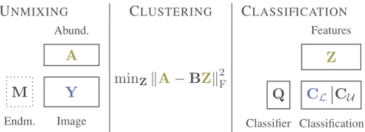
Fig. 1. Structure of the cofactorization model. Variables inbluestand for observations or available external data. Variables in olive greenare linked through the clustering term. The variable in a dotted box is assumed to be known beforehand.
C. Clustering
To define a global cofactorization problem, a relation is drawn between the activation matrices of the two factorization problems, namely the abundance matrix and the feature matrix. More specifically, following the idea developed in [8], a clus-tering term is introduced as a coupling. Abundances vectors are clustered and the resulting attribution vectors are then used as feature vectors for the classification. Ideally, clustering attribution vectors zp ∈ RK are filled with zeros except for
zk,p= 1 when apis associated with the kth cluster. The
well-known k-means is chosen to perform this task since it is easily expressed as an optimization problem
min Z,B 1 2&A − BZ& 2 F+ ıSP K(Z) + ıR R×K + (B) (7)
where columns of B ∈ RR×K stands for the centroids of
the K clusters. Two constraints are considered in this k-means clustering problem: i) a positivity constraint on B since centroids are expected to be interpretable as mean abundance vectors and ii) the vectors zp (p ∈ P) are assumed to be
defined on the K-dimensional probability simplex SK. Thus,
the resulting clustering method is a particular instance of k-means where the attribution vectors are relaxed and can be interpreted as the collection of probabilities to belong to each of the clusters.
D. Multi-objective problem
The two factorization problems corresponding to the spec-tral unmixing and classification tasks have been expressed and the link between these two problems has been set up through the clustering term. The global cofactorization problem, illus-trated in Figure 1, is finally formulated as
min A,Q,Z CU,B λ0 2 &Y − MA& 2 F+ λa&A&1+ ıRR×P + (A) −λ1 2 ! p∈P dp ! i∈C ci,plog # 1 1 + exp(−qi:zp) $ +λq 2 &Q& 2 F+ λc&C&vTV+ ıS|U |C (CU) +λ2 2 &A − BZ& 2 F + ıSP K(Z) + ıR R×K + (B) (8)
where λ0, λ1and λ2are introduced to weight the contribution
of the various terms.
III. OPTIMIZATION SCHEME
The proposed global optimization problem (8) is non-convex and non-smooth. Such problem are usually very chal-lenging to solve. To handle it, we propose to resort to the PALM algorithm proposed in [9]. PALM algorithm ensures convergence to a critical point, i.e., a local minimum of the ob-jective function. To apply PALM, the obob-jective is rewritten as a sum of independent non-smooth terms fj(·) (j ∈ {1, . . . , 3})
and a smooth coupling term g(·) min
A,B,Z, Q,CU
f0(A)+f1(B)+f2(Z)+f3(CU)+g(A, B, Z, CU, Q)
where
f0(A) = ıR+(A) + λa&A&1, f1(B) = ıR+(B)
f2(Z) = ıSP K(Z), f3(CU) = ıS|U |K (CU) g(A, B, Z, CU, Q) = λ0 2 &Y − MA& 2 F −λ1 2 ! p∈P dp ! i∈C ci,plog # 1 1 + exp(−qi:zp) $ +λ2 2 &A − BZ& 2 F+ λq 2 &Q& 2 F+ λc&C&vTV. Algorithm 1: PALM
1 Initialize variables A0, B0, Z0, CU0and Q0; 2 Set α >1;
3 while stopping criterion not reached do 4 Ak+1∈ proxαLA f0 (A k− 1 αLA∇Ag(A k, Bk, Zk, Ck U, Q k)); 5 Bk+1∈ proxαLB f1 (B k− 1 αLB∇Bg(A k+1, Bk, Zk, Ck U, Qk)); 6 Zk+1∈ proxαLZ f2 (Z k− 1 αLZ∇Zg(A k+1, Bk+1, Zk, Ck U, Qk)); 7 Qk+1∈ proxαLQ f3 (Q k− 1 αLQ∇Qg(A k+1, Bk+1, Zk+1, C Uk, Qk)); 8 Ck+1U ∈ prox αLCU f4 (C k U− 1 αLCU∇CUg(Ak+1, Bk+1, Zk+1, C k U, Qk+1)); 9 end
10 return Aend, Bend, Zend, Qend, Cend
U
The concept of this algorithm is to perform a proximal gradient descent according to each variable alternatively. To apply PALM, the functions fj(·) have to be proper, lower
semi-continuous, extended real-valued. A sufficient condition on the function g(·) is to be C2, i.e., with continuous first
and second derivatives, and its partial gradients have to be globally Lipschitz. LX denotes herein the Lipschitz constant
associated to the partial gradient according to X. The detailed steps of the algorithm are summarized in Algorithm 1 and further theoretical details are available in [9].
In practice, one needs to be able to compute the partial gradient and its associated Lipschitz constant to perform the gradient descent. It is also necessary to compute the proximal operator associated to the non-smooth terms. In the present case, the partial gradients is easily computed and all globally Lipschitz. The only problematic term is the vTV term which is not globally Lipschitz in its canonical form. To alleviate,
a smoothed counterpart has been introduced in (6) with a smoothing parameter ǫ∈ R+. As for the proximal operators,
they are are well-known [12] except for f0(·). For f0(·), it
is necessary to resort to the composition of the proximal operators associated to the non-negative constraint and the ℓ1
-norm, which is here possible according to [13]. IV. EXPERIMENTS
Data generation – The HSI used to perform the experiments is a semi-synthetic image. More specifically, the image has been generated using a real HSI. The real image has been unmixed using a fully constrained least square (FCLS) algorithm [14] using R= 5 endmembers extracted with the well-known VCA algorithm [15]. The obtained abundance maps have then been used to generate a new synthetic image using pure spectra from the hyperspectral library ASTER [16]. The groundtruth of the original data, composed of C = 3 classes has been preserved to assess the quality of the classification. A color composition, a panchromatic version and the groundtruth are presented in Figure 2. The subset of the image used as training data is as also shown in Figure 2.
(a) (b) (c) (d)
Fig. 2. Synthetic image: (a) colored composition of the HSI Y, (b) panchromatic image yPAN, (c) classification ground-truth, (d) training set.
Initialization and convergence – As stated before, cofac-torization is a non-convex problem and PALM only ensures convergence to a local minimum of the objective function. It is thus important to carefully initialize the estimated vari-ables in order to reach a relevant solution. In the presented experiment, abundance matrix A0 has been initialized by solvingminA∈RR×P
+ &Y − MA&
2
F using a projected gradient
algorithm. Then, a k-means algorithm has been applied to the obtained abundance vectors and the resulting centroids and attribution vectors have been used to initialize B0 and Z0. On the other hand, classifier parameters Q0and classification matrix C0U have been initialized randomly.
In order to assess the convergence of the optimization scheme, the normalized difference between two consecutive values of the objective function is monitored. When this value reach a certain threshold (10−4for this experiment), the
optimization process stops and the last estimation is assumed to be close enough to the solution.
Hyperparameters – Multiple hyperparameters λ· have been
introduced in problem (8) to weight the various terms of the objective function. For practical use, these parameters have been normalized by the size and dynamics of the cor-responding variables. These normalized parameters, denoted
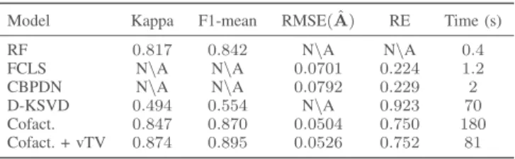
TABLE I
UNMIXING AND CLASSIFICATION RESULTS.
Model Kappa F1-mean RMSE( ˆA) RE Time (s)
RF 0.817 0.842 N\A N\A 0.4 FCLS N\A N\A 0.0701 0.224 1.2 CBPDN N\A N\A 0.0792 0.229 2 D-KSVD 0.494 0.554 N\A 0.923 70 Cofact. 0.847 0.870 0.0504 0.750 180 Cofact. + vTV 0.874 0.895 0.0526 0.752 81 ˜
λ·, have been empirically tuned to obtain consistent results
(˜λ0 = ˜λ1 = ˜λ2 = 1, ˜λa = 10−3, ˜λq = 0.15). For the last
hyperparameter ˜λc, two values have been considered 0. and
0.1, standing respectively for the case without and with spatial regularization. The definition of the vTV regularization also includes parameters which has to be properly set. First, the smoothing parameter is set to ǫ= 0.01 to ensure the gradient-Lipschitz property without modifying substantially the TV-norm. Secondly, it is necessary to define the weighing coeffi-cients βm,n. They have been computed from a panchromatic
image yPAN, shown in Figure 2, generated by normalizing
hyperspectral bands by their mean and then summing them. More precisely, to account for possible homogeneous areas in the image, they are defined as follows
βp= ˜ βp ' qβ˜q with ˜βq = (& & &[∇yPAN]q & & & 2+ σ )−1
where σ = 0.01 controls the variation of the weights and avoids numerical issues.
Compared methods – To assess the quality of the unmix-ing and classification results, the proposed method has been compared to several well-known unmixing and classification algorithms. Regarding classification, we considered the ran-dom forest (RF) algorithm, known to perform very well to classify HSI. Parameters of the RF (number of trees, depth) have been adjusted using gridsearch and cross-validation. The discriminative K-SVD (D-KSVD) method has been used as a benchmark [17]. This model is also a cofactorization method but with a simpler approach where the two coding matrices A and Z are imposed to be equal. In this case, the first term is not a spectral unmixing task but rather a dictionary learning task where dictionary elements are assumed to be discriminative for the classification task. Only a sparsity penalization is considered for D-KSVD using a ℓ0-norm.
As for the unmixing comparison, we considered two meth-ods described in [14]. The first method is the fully constrained least square method (FCLS) where the corresponding opti-mization problem is defined as the data fitting term with a positivity and sum-to-one constraint on abundance vectors ap.
The second method is the constrained basis pursuit denoising (CBPDN) corresponding to problem 1. The hyperparameter λa, weighting the sparsity penalty is also adjusted using
gridsearch and cross-validation. It should be noted that all unmixing methods use directly the correct endmember matrix M which has been used to generate the data. Additionally, the endmember matrix is used to initialize the dictionary of the D-KSVD method.
Results – To evaluate the unmixing results quantitatively, the reconstruction error (RE) and root global mean squared error (RMSE) are considered, i.e.,
RE = % 1 P L & & &Y− M ˆA & & & 2 F,RMSE = % 1 P R & & &Atrue− ˆA & & & 2 F,
where Atrue and ˆA are the actual and estimated abundance
matrices. To evaluate the classification accuracy, two con-ventional metrics are used, namely Cohen’s kappa coefficient and the averaged F1-score over all classes [18]. The results have been averaged over 20 trials. A different random noise has been added to the image for each trial such that the SNR= 30dB. 0 100 200 300 Band Blue class 0 100 200 300 Band Brown class 0 100 200 300 Band Cyan class
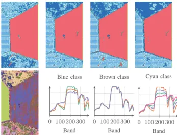
Fig. 3. Results: (1st row) classification maps for D-KSVD, RF, Cofact., Cofact. + vTV, (2nd row) cluster map and spectral centroids recovered by the proposed method (Cofact. + vTV).
Results reported in Table I show that the proposed co-factorization framework outperforms both RF and D-KSVD in term of classification. Regarding spectral unmixing, FCLS and CBPDN reach lower REs which is expected since both methods exhibit more degrees of freedom. Note however this metrics only evaluates the quality of the reconstructed data. However, RMSE is lower for the cofactorization methods than for FCLS and CBPDN. It is finally interesting to underline the improvement due to the vTV. As expected, classification results improve when the spatial regularization is considered but additionally the convergence time of the PALM algorithm is significantly reduced. Processing time is indeed higher for the proposed cofactorization method than for RF, FCLS and CBPDN. However, it simultaneously tackles two problems instead of one, and processing time still remains comparable to the one of D-KSVD method.
In terms of qualitative results, Figure 3 presents the clas-sification maps which appear consistent with the quantitative results. Moreover, results of the clustering task are shown with spectral centroids of the clusters for each classes. In particular, this cluster maps exhibits some heterogeneity, which can be explained by the multi-modality of some classes. This additional result is a very interesting byproduct of the proposed method to interpret the scene.
V. CONCLUSION AND PERSPECTIVE
This paper introduces a unified framework to perform jointly spectral unmixing and classification by the mean of a cofactorization problem. Coding matrices of two problems of interest are linked thanks to a clustering term. The over-all cofactorization task is formulated as a convex non-smooth optimization problem whose solution was approx-imated thanks to a PALM algorithm which ensured some convergence guarantees. Even if the proposed method appears to perform significantly well compared to other state-of-the-art methods, further improvements are yet to be considered. In particular, the additional learning of the endmember matrix could be considered. It would be also relevant to exploit the supervised information on the spectral unmixing part which is very rarely available in a conventional unmixing problem.
REFERENCES
[1] Y. Chen, H. Jiang et al., “Deep feature extraction and classification of hyperspectral images based on convolutional neural networks,” IEEE
Trans. Geosci. Remote Sens., vol. 54, no. 10, pp. 6232–6251, 2016. [2] M. Belgiu and L. Dr˘agut¸, “Random forest in remote sensing: A review
of applications and future directions,” ISPRS Journal of Photogrammetry
and Remote Sensing, vol. 114, pp. 24–31, 2016.
[3] J. M. Bioucas-Dias, A. Plaza et al., “Hyperspectral Unmixing Overview: Geometrical, Statistical, and Sparse Regression-Based Approaches,”
IEEE J. Sel. Topics Appl. Earth Observ. in Remote Sens., vol. 5, no. 2, pp. 354–379, April 2012.
[4] A. Villa, J. Chanussot et al., “Spectral unmixing for the classification of hyperspectral images at a finer spatial resolution,” IEEE J. Sel. Top.
Signal Process., vol. 5, no. 3, pp. 521–533, 2011.
[5] I. D´opido, J. Li et al., “A new hybrid strategy combining semisupervised classification and unmixing of hyperspectral data,” IEEE J. Sel. Topics
Appl. Earth Observ. in Remote Sens., vol. 7, no. 8, pp. 3619–3629, 2014. [6] J. Yoo, M. Kim et al., “Nonnegative matrix partial co-factorization for drum source separation,” in Acoustics Speech and Signal Processing
(ICASSP), 2010 IEEE International Conference On. IEEE, 2010, pp. 1942–1945.
[7] N. Yokoya, T. Yairi et al., “Coupled nonnegative matrix factorization unmixing for hyperspectral and multispectral data fusion,” IEEE Trans.
Geosci. Remote Sens., vol. 50, no. 2, pp. 528–537, 2012.
[8] A. Lagrange, M. Fauvel et al., “Hierarchical Bayesian image analysis: From low-level modeling to robust supervised learning,” Pattern
Recog-nit., vol. 85, pp. 26–36, 2019.
[9] J. Bolte, S. Sabach et al., “Proximal alternating linearized minimization for nonconvex and nonsmooth problems,” Mathematical Programming, vol. 146, no. 1-2, pp. 459–494, Aug. 2014.
[10] I. Goodfellow, Y. Bengio et al., Deep Learning. MIT press Cambridge, 2016, vol. 1.
[11] T. Uezato, M. Fauvel et al., “Hyperspectral image unmixing with LiDAR data-aided spatial regularization,” IEEE Trans. Geosci. Remote Sens., 2018.
[12] L. Condat, “Fast projection onto the simplex and the l1 ball,” Math.
Program., vol. 158, no. 1-2, pp. 575–585, 2016.
[13] Y.-L. Yu, “On decomposing the proximal map,” in Adv. Neural Inf.
Process. Syst., 2013, pp. 91–99.
[14] J. M. Bioucas-Dias and M. A. Figueiredo, “Alternating direction algo-rithms for constrained sparse regression: Application to hyperspectral unmixing,” in Proc. IEEE Workshop Hyperspectral Image SIgnal
Pro-cess.: Evolution in Remote Sens. (WHISPERS). IEEE, 2010, pp. 1–4. [15] J. M. P. Nascimento and J. M. Bioucas-Dias, “Vertex component analysis: A fast algorithm to unmix hyperspectral data,” IEEE Trans.
Geosci. Remote Sens., vol. 43, no. 4, pp. 898–910, April 2005. [16] A. M. Baldridge, S. J. Hook et al., “The ASTER spectral library version
2.0,” Remote Sens. Environ., vol. 113, no. 4, pp. 711–715, 2009. [17] Z. Jiang, Z. Lin et al., “Learning a discriminative dictionary for sparse
coding via label consistent K-SVD,” in CVPR 2011, June 2011, pp. 1697–1704.
[18] R. G. Congalton and K. Green, Assessing the Accuracy of Remotely