Hyperspectral Pansharpening: A Review

(1)

To cite this version : Loncan, Laetitia and Almeida, Luis B. and

Bioucas-Dias, José M. and Briottet, Xavier and Chanussot, Jocelyn and

Dobigeon, Nicolas and Fabre, Sophie and Liao, Wenzhi and Licciardi,

Giorgio A. and Simoes, Miguel and Tourneret, Jean-Yves and

Veganzones, Miguel Angel and Vivone, Gemine and Wei, Qi and

Yokoya, Naoto

Hyperspectral Pansharpening: A Review

. (2015) IEEE

Geoscience and Remote Sensing Magazine, vol. 3 (n° 3). pp. 27-46.

ISSN 2168-6831

To link to this article : doi: 10.1109/MGRS.2015.2440094

URL :

http://dx.doi.org/10.1109/MGRS.2015.2440094

O

pen

A

rchive

T

OULOUSE

A

rchive

O

uverte (

OATAO

)

OATAO is an open access repository that collects the work of Toulouse researchers and

makes it freely available over the web where possible.

This is an author-deposited version published in :

http://oatao.univ-toulouse.fr/

Eprints ID : 14340

Any correspondance concerning this service should be sent to the repository

administrator:

[email protected]

(2)

Hyperspectral Pansharpening:

A Review

LAETITIA LONCAN

Gipsa-lab, Grenoble, France and ONERA, Toulouse, France (e-mail: [email protected])

LUÍS B. ALMEIDA AND JOSÉ M. BIOUCAS-DIAS Instituto de Telecomunicações, Instituto Superior Técnico, Universidade de Lisboa

(e-mails: [email protected], [email protected]) XAVIER BRIOTTET

ONERA, Toulouse, France (e-mail: [email protected]) JOCELYN CHANUSSOT Gipsa-lab, Grenoble, France

(e-mail: [email protected]) NICOLAS DOBIGEON

University of Toulouse, IRIT/INP-ENSEEIHT (e-mail: [email protected])

SOPHIE FABRE

ONERA, Toulouse, France (e-mail: [email protected]) WENZHI LIAO

Ghent University, Ghent, Belgium (e-mail: [email protected]) GIORGIO A. LICCIARDI

Gipsa-lab, Grenoble, France (e-mail: Giorgio-Antonino. [email protected])

MIGUEL SIMÕES

Instituto de Telecomunicações, Instituto Superior Te´cnico, Universidade de Lisboa and Gipsa-lab, Grenoble, France (e-mail: [email protected])

JEAN-YVES TOURNERET

(3)

Abstract_{—Pansharpening aims at fusing a panchromatic}

image with a multispectral one, to generate an image with the high spatial resolution of the former and the high spectral resolution of the latter. In the last decade, many algorithms have been presented in the literatures for pansharpen-ing uspansharpen-ing multispectral data. With the increasing availabil-ity of hyperspectral systems, these methods are now be-ing adapted to hyperspec-tral images. In this work, we compare new pansharpening techniques designed for hy-perspectral data with some of the state-of-the-art meth-ods for multispectral pan-sharpening, which have been adapted for hyperspectral data. Eleven methods from different classes (component substitution, multiresolution analysis, hybrid, Bayesian and matrix factorization) are analyzed. These methods are ap-plied to three datasets and their effectiveness and robust-ness are evaluated with widely used performance indicators. In addition, all the pansharpening techniques considered in this paper have been implemented in a MATLAB toolbox that is made available to the community.

I. INTRODUCTION

I

n the design of optical remote sensing systems, owing to the limited amount of incident energy, there are criti-cal tradeoffs between the spatial resolution, the spectral resolution, and signal-to-noise ratio (SNR). For this rea-son, optical systems can provide data with a high spatial resolution but with a small number of spectral bands (for example, panchromatic data with decimetric spatial reso-lution or multispectral data with three to four bands and metric spatial resolution, like PLEIADES [1]) or with a high spectral resolution but with reduced spatial resolution (for example, hyperspectral data, subsequently referred to as HS data, with more than one hundred of bands and deca-metric spatial resolution like HYPXIM [2]). To enhance the spatial resolution of multispectral data, several methods have been proposed in the literature under the name of pansharpening, which is a form of superresolution.

Fun-damentally, these methods solve an inverse problem which consists of obtaining an enhanced image with both high spatial and high spectral resolutions from a panchromatic image and a multispectral image. The huge interest of the community on this topic is evidenced by the existence of sessions dedicated to this topic in the most important re-mote sensing and earth observation conferences as well as by the launch of public contests, of which the one spon-sored by the data fusion committee of the IEEE Geoscience and Remote Sensing society [3] is an example.

A taxonomy of pansharpening methods can be found in the literature [4], [5], [6]. They can be broadly divided into four classes: component substitution (CS), multi-resolution analysis (MRA), Bayesian, and variational. The CS approach relies on the substitution of a component (obtained, e.g., by a spectral transformation of the data) of the multispectral (subsequently denoted as MS) image by the panchromatic (subsequently denoted as PAN) im-age. The CS class contains algorithms such as intensity-hue-saturation (IHS) [7], [8], [9], principal component analysis (PCA) [10], [11], [12] and Gram-Schmidt (GS) spectral sharpening [13]. The MRA approach is based on the injection of spatial details, which are obtained through a multiscale decomposition of the PAN image into the MS data. The spatial details can be extracted ac-cording to several modalities of MRA: decimated wavelet transform (DWT) [14], undecimated wavelet transform (UDWT) [15], “à-trous” wavelet transform (ATWT) [16], Laplacian pyramid [17], nonseparable transforms, either based on wavelets (e.g., curvelets [19]) or not (e.g., con-tourlets [18]). Hybrid methods have been also proposed, which use both component substitution and multiscale decomposition, such as guided filter PCA (GFPCA), de-scribed in Section II-C. The Bayesian approach relies on the use of posterior distribution of the full resolution tar-get image given the observed MS and PAN images. This posterior, which is the Bayesian inference engine, has two factors: a) the likelihood function, which is the probabil-ity densprobabil-ity of the observed MS and PAN images given the target image, and b) the prior probability density of the target image, which promotes target images with desired properties, such as being segmentally smooth. The selec-tion of a suitable prior allows us to cope with the usual ill-posedness of the pansharpening inverse problems. The variational class is interpretable as particular case of the

MIGUEL A. VEGANZONES Gipsa-lab, Grenoble, France (e-mail: miguelangel.veganzones @gipsa-lab.grenoble-inp.fr) GEMINE VIVONE

North Atlantic Treaty Organization (NATO) Science and Technology Organization (STO) Centre

for Maritime Research and Experimentation (CMRE) (e-mail: [email protected])

QI WEI

NAOTO YOKOYA University of Tokyo

(e-mail:[email protected])

FUSING IMAGES WITH COMPLEMENTARY PROPERTIES,

PANSHARPENING HELPS SYNTHETIZING A HYPERSPECTRAL IMAGE WITH A HIGH SPATIAL RESOLUTION.

(4)

Bayesian one, where the target image is esti-mated by maximizing the posterior probabil-ity densprobabil-ity of the full resolution image. The works [20], [21], [22] are representative of the Bayesian and variational classes. As indicated in Table 1, the CS, MRA, and Hybrid classes of methods are detailed in Sections A, II-B, and II-C, respectively. Herein, the Bayesian class is not addressed in the MS+PAN context. It is addressed in detail, however, in Section II-D in the context of HS+PAN fusion.

With the increasing availability of HS sys-tems, the pansharpening methods are now ex-tended to the fusion of HS and panchromatic images [23], [24], [25], [26]. Pansharpening of HS images is still an open issue, and very few methods are presented in the literature to

ad-dress it. The main advantage of HS image with respect to MS one is the more accurate spectral information they provide, which clearly benefits many applications such as unmixing [27], change detection [28], object recognition [29], scene interpretation [30] and classification [31]. Several of the methods designed for HS pansharpening were originally designed for the fusion of MS and HS data[32]–[36], the MS data constituting the high spatial resolution image. In this case, HS pansharpening can be seen as a particular case, where the MS image is composed of a single band, and thus reduces to a PAN image. In this paper, we divide these meth-ods into two classes: Bayesian methmeth-ods and matrix factor-ization based methods. In Section II-D, we briefly present the algorithms of [33], [36], and [35] of the former class and in Section II-E the algorithm of [32] of the latter class.

As one may expect, performing pansharpening with HS data is more complex than performing it with MS data. Whereas PAN and MS data are usually acquired almost in the same spectral range, the spectral range of an HS image normally is much wider than the one of the correspond-ing PAN image. Usually, the PAN spectral range is close to the visible spectral range of 0.4−0.8nm (for example, the advanced land imager–ALI–instrument acquires PAN data in the range 0.48−0.69nm). The HS range often covers the visible to the shortwave infrared (SWIR) range (for exam-ple, Hyperion acquires HS data in the range 0.4−2.5nm, the range 0.8−2.5nm being not covered by the PAN data). The difficulty that arises, consists in defining a fusion model that yields good results in the part of the HS spectral range that is not covered by PAN data, in which the high resolu-tion spatial informaresolu-tion is missing. This difficulty already existed, to some extent, in MS+PAN pansharpening, but it is much more severe in the HS+PAN case.

To the best of the authors’ knowledge, there is currently no study comparing different fusion methods for HS data, particularly on datasets where the spectral domain of the HS image is larger than the one of the PAN image. This work aims at addressing this specific issue. The remainder of the paper is organized as follows. Section II reviews the

methods under study, i.e., CS, MRA, hybrid, Bayesian, and matrix decomposition approaches. Section III summarizes the quality assessment measures that will be used to assess the image fusion results. Experimental results are presented in Section IV. Conclusions are drawn in Section V.

II. HYPERSPECTRAL PANSHARPENING TECHNIQUES

This section presents some of the most relevant methods for HS pansharpening. First, we focus on the adaptation of the popular CS and MRA MS pansharpening methods for HS pansharpening. Later, we consider more recent methods based on Bayesian and matrix factorization approaches. A toolbox containing MATLAB implementations of these al-gorithms can be found online1_.

Before presenting the different methods, we introduce notation used along the paper. Bold-face capital letters refer to matrices and bold-face lower-case letters refer to vectors. The notation Xk

refers to the thk _{row of X. The operator ()}T

denotes the transposition operation. Images are represent-ed by matrices, in which each row corresponds to a spec-tral band, containing all the pixels of that band arranged in lexicographic order. We use the following specific matrices:

◗ _X x, ,xn _R m n

1f !

=6 @ m# _{represents the full resolution}

target image with mm bands and n pixels; XW represents

an estimate of that image. ◗ _YH _R , m m ! m# YM _R , n n ! m# and P R1 n ! # represents, re-spectively, the observed HS, MS, and PAN images, nm denoting the number of bands of the MS image and m the total number of pixel in the YH image.

◗ L_YH_!_Rmm#n

represents the HS images YH interpolated at the scale of the PAN image.

We denote by d₌ m n/ the down-sampling factor, as-sumed to be the same in both spatial dimensions.

A. COMPONENT SUBSTITUTION

CS approaches rely upon the projection of the higher spectral resolution image into another space, in order to

1_{http://openremotesensing.net}

TABLE 1. SUMMARY OF THE DIFFERENT CLASSES OF METHODS CONSIDERED IN THIS PAPER. WITHIN PARENTHESES, WE INDICATE THE ACRONYM OF EACH METHOD, FOLLOWED BY THE NUMBER OF THE SECTION IN WHICH THAT METHOD IS DESCRIBED.

METHODS ORIGINALLY DESIGNED FOR MS PANSHARPENING Component substitution (CS, II-A)

Principal Component Analysis (PCA, II-A-1) Gram Schmidt (GS, II-A-2)

Multiresolution analysis (MRA, II-B) Smoothing filter-based intensity modulation (SFIM, II-B-1) Laplacian pyramid (II-B-2) Hybrid methods (II-C)

Guided Filter PCA (GFPCA)

Bayesian methods Not discussed in this paper METHODS ORIGINALLY DESIGNED FOR HS PANSHARPENING Bayesian Methods (II-D)

Naive Gaussian prior (II-D-1) Sparsity promoting prior (II-D-2) HySure (II-D-3)

Matrix Factorization (II-E) Coupled Non-negative Matrix Factorization (CNMF)

(5)

separate spatial and spectral information [6]. Subsequent-ly, the transformed data are sharpened by substituting the component that contains the spatial information with the PAN image (or part of it). The greater the correlation be-tween the PAN image and the replaced component, the less spectral distortion will be introduced by the fusion approach [6]. As a consequence, a histogram-matching procedure is often performed before replacing the PAN im-age. Finally, the CS-based fusion process is completed by applying the inverse spectral transformation to obtain the fused image.

The main advantages of the CS-based fusion techniques are the following: i) high fidelity in rendering the spatial details in the final image [37], ii) fast and easy implemen-tation [8], and iii) robustness to misregistration errors and aliasing [38]. On the negative side, the main shortcoming of this class of techniques is the generation of a significant spectral distortion, cause by the spectral mismatch between the PAN and the HS spectral ranges [6].

Following [4], [39], a formulation of the CS fusion scheme is given by , Xk =YLHk+gk^P-OLh W (1) for k=1,f,mm, where X k

W denotes the thk band of the es-timated full resolution target image, g g, ,gm

T

1f

=6 m@ is a

vector containing the injection gains, and OL is defined as

, OL wYH i m i i 1 = = m L

/

(2)

where the weights w w , ,wi, ,wm T

1f f

=6 m@ measure the

spectral overlap among the spectral bands and the PAN im-age [6], [40].

The CS family includes many popular pansharpening approaches. In [26], three approaches based on principal

component analysis (PCA) [9] and Gram-Schmidt [13], [37]

transformations have been compared for sharpening HS data. A brief description of these techniques follows.

1) Principal Component Analysis: PCA is a spectral

trans-formation widely employed for pansharpening applica-tions [9]. It is achieved through a rotation of the original data (i.e., a linear transformation) that yields the so-called principal components (PCs). The hypothesis underlying its application to pansharpening is that the spatial infor-mation (shared by all the channels) is concentrated in the first PC, while the spectral information (specific to each single band) is accounted for the other PCs. The whole fu-sion process can be described by the general formulation stated by Eqs. (1) and (2), where the vectors w and g of coefficient vectors are derived by the PCA procedure ap-plied to the HS image.

2) Gram-Schmidt: The Gram-Schmidt transformation,

of-ten exploited in pansharpening approaches, was initially proposed in a patent by Kodak [13]. The fusion process starts by using, as the component, a synthetic low resolu-tion PAN image IL at the same spatial resolution as the HS

image2_{. A complete orthogonal decomposition is then}

per-formed, starting with that component. The pansharpening procedure is completed by substituting that component with the PAN image, and inverting the decomposition. This process is expressed by (1) using the gains [37]

, var cov O Y O gk H L k L = ^ ^ h h L (3)

for k=1,f,mm, where cov ,^ h$ $ and var $^ h denote the co-variance and co-variance operations. Different algorithms are obtained by changing the definition of the weights in (2). The simplest way to obtain this low-resolution PAN image simply consists of averaging the HS bands (i.e., by setting

/ ,

wi₌1mm for i=1,f,mmh. In [37], the authors proposed

an enhanced version, called GS Adaptive (GSA), in which

IL is generated by the linear model in (2) with weights es-timated by the minimization of the mean square error be-tween the estimated component and a filtered and downs-ampled version of the PAN image.

B. MULTIRESOLUTION ANALYSIS

Pansharpening methods based on MRA apply a spatial fil-ter to the PAN image for generating details to be injected into the HS data. The main advantages of the MRA-based fusion techniques are the following: i) temporal coher-ence [5] (see Sect.27.4.4), ii) spectral consistency, and iii) robustness to aliasing, under proper conditions [38]. On the negative side, the main shortcomings are i) the imple-mentation is more complicated due to the design of spatial filters, ii) the computational burden is usually larger when compared to CS approaches. The fusion step is summa-rized as [4], [39] , X YH G P P k k k7 L =L + ^ - h W (4)

for k=1,f,mm, where PL denotes a low-pass version of P,

and the symbol 7 denotes element-wise multiplication. Furthermore, an equalization between the PAN image and the HS spectral bands is often required. P-PL is often

called the details image, because it is a high-pass version of

P, and Eq. (4) can be seen as describing the way to inject

details into each of the bands of the HS image. According to (4), the approaches belonging to this category can differ in i) the type of PAN low pass image PL that is used, and

iih_{the definition of the gain coefficients G .}k Two common

options for defining the gains are:

1) Gk_{= for}1 k=1,f,mm, where 1 is an appropriately

sized matrix with all elements equal to 1. This choice identifies the so-called additive injection scheme; 2) Gk YH P

k L

8

= L for k=1,f,mm, where the symbol 8

de-notes element-wise division. In this case, the details are weighted by the ratio between the upsampled HS im-age and the low-pass filtered PAN one, in order to re-produce the local intensity contrast of the PAN image 2_{GS is a more general method than PCA. PCA can be obtained, in GS, by}

(6)

in the fused image [42]. This coefficient selection is of-ten referred to as high pass modulation (HPM) method or

multiplicative injection scheme. Some possible numerical

issues could appear due to the division between YH

k

L and

PL for low value of PL creating fused pixel with very high

value. In our toolbox this problem is addressed by clip-ping these values by using the information given by the dynamic range.

In the case of HS pansharpening, some further consid-erations should be taken into account. Indeed, the PAN and HS images are rarely acquired with the same platform. Thus, the ratio between the spatial resolutions of the PAN and HS images may not always be an integer number, or a power of two. This implies that some of the conventional approaches initially developed for MS images cannot be extended in a simple way to HS images (for example, dyadic wavelet-based algorithms cannot be applied in these conditions).

1) Smoothing Filter-based Intensity Modulation (SFIM): The

direct implementation of Eq. (4) consists of applying a sin-gle linear time-invariant (LTI) low pass filter (LPF) hLP to the PAN image P for obtaining P .L Therefore, we have

X YH g P P hLP

k k

k )

=L + ^ - h

W (5)

for k=1,f,mm, where the symbol ) denotes the convolu-tion operator. The SFIM algorithm [43] sets hLP to a simple

box (i.e., an averaging) filter and exploits HPM as the de-tails injection scheme.

2) Laplacian Pyramid: The low-pass filtering needed to

obtain the signal PL at the original HS scale can be

per-formed in more than one step. This is commonly referred to as pyramidal decomposition and dates back to the semi-nal work of Burt and Adelson [17]. If a Gaussian filter is used to lowpass filter the images in each step, one obtains a so-called Gaussian pyramid. The differences between con-secutive levels of a Gaussian pyramid define the so-called

Laplacian pyramid. The suitability of the latter to the

pan-sharpening problem has been shown in [44]. Indeed, Gaussian filters can be tuned to closely match the sen-sor modulation transfer function (MTF). In this case, the unique parameter that characterizes the whole distribution is the Gaussian’s standard deviation, which is determined from sensor-based information (usually from the value of the amplitude response at the Nyquist frequency, provided by the manufacturer). Both additive and multiplicative details injection schemes have been used in this framework [42], [45]. They will be referred to as MTF-Generalized Laplacian

Pyramid (MTF-GLP) [45] and MTF-GLP with High Pass Modu-lation (MTF-GLP-HPM) [42], respectively.

C. HYBRID METHODS

Hybrid approaches use concepts from different classes of methods, namely from CS and MRA ones, as explained next.

1) Guided Filter PCA (GFPCA): One of the main

challeng-es for fusing low-rchalleng-esolution HS and high-rchalleng-esolution PAN/ RGB data is to find an appropriate balance between spectral

and spatial preservation. Recently, the guided filter [46] has been used in many applications (e.g. edge-aware smooth-ing and detail enhancement), because of its efficiency and strong ability to transfer the structures of the guidance im-age to the filtering output. Its application to HS data can be found in [47], where the guided filter was applied to trans-fer the structures of the principal components of the HS im-age to the initial classification maps.

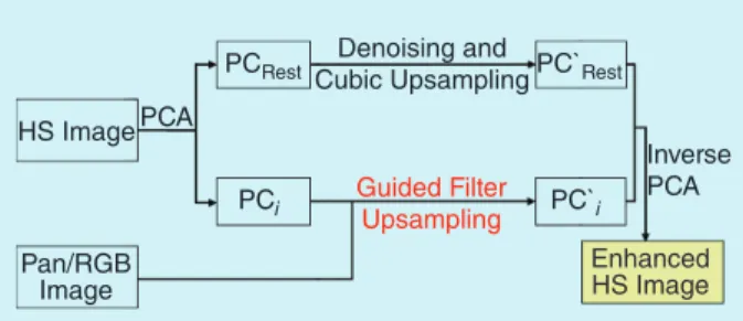
Here, we briefly describe an image fusion framework which uses a guided filter in the PCA domain (GFPCA) [48]. The approach won the “Best Paper Challenge” award at the 2014 IEEE data fusion contest [48], by fusing a low spatial resolution thermal infrared HS image and a high spatial resolution, visible RGB image associated with the same scene. Fig. 1 shows the framework of GFPCA. In-stead of using CS, which

may cause spectral distor-tions, GFPCA uses a high resolution PAN/RGB image to guide the filtering process aimed at obtaining super-resolution. In this way, GF-PCA does not only preserve the spectral information from the original HS im-age, but also transfers the spatial structures of the high resolution PAN/RGB image to the enhanced HS image. To speed up the processing, GFPCA first uses PCA to decorrelate the bands of the

HS image, and to separate the information content from the noise. The first p_%mm PCA channels contain most of

the energy (and most of the information) of an HS image, and the remaining mm_-p PCA channels mainly contain

noise (recall that mm is the number of spectral bands of the

HS image). When applied to these noisy (and numerous)

mm_-p channels, the guided filter amplifies the noise and

causes a high computational cost in processing the data, which is undesirable. Therefore, guided filtering is used to enlarge only the first k PCA channels, preserving the structures of the PAN/RGB image, while cubic interpola-tion is used to upsample the remaining channels.

FIGURE 1. Fusion of HS and PAN/RGB images with the GFPCA framework. Denoising and Cubic Upsampling HS Image Pan/RGB Image PC_i PC`_i PC`_Rest PC_Rest PCA Inverse PCA Guided Filter Upsampling Denoising and Cubic Upsampling HS Image Pan/RGB Image PC_i PC`_i PC`_Rest PC_Rest PCA Inverse PCA Guided Filter Upsampling Enhanced HS Image

DERIVED FROM THE STANDARD

PANSHARPENING

LITERATURE, COMPONENT SUBSTITUTION,

MULTIRESOLUTION ANALYSIS AND HYBRID METHODS ARE THE THREE MAIN CLASSES OF METHODS.

(7)

Let PC ,i with ^i_#ph, denote the thi PC channel

ob-tained from the HS image Y ,H with its resolution increased to that of the guided image Y ( Y may be a PAN or an RGB image) through bicubic interpolation. The output of the filtering, PCil, can be represented as an affine transforma-tion of Y in a local window ~j of size ^2d₊1h#^2d₊1h as follows:

Y , .

PCil=aj +bj 6 ! ~i j (6)

The above model ensures that the output PCil has an edge

only if the guided image Y has an edge, since d^PCilh₌ad_Y. The following cost function is used to determine the coef-ficients aj and :bj PC Y ( , ) ( ) , E a bj j aj bj i aj i 2 2 j e = + - + ! ~ 6 @

/

(7)

where e is a regularization parameter determining the de-gree of blurring for the guided filter. For more details about the guided filtering scheme, we invite the reader to consult [46]. The cost function E leads the term Yaj +bj to be as

close as possible to PCi, in order to ensure the preservation of the original spectral information. Before applying in-verse PCA, GFPCA also removes the noise from the remain-ing PCA channels PCRest using a soft-thresholding scheme

(similarly to [49]), and increases their spatial resolution to the resolution of the PAN/RGB image using cubic interpola-tion only (without guided filtering).

D. BAYESIAN APPROACHES

The fusion of HS and high spatial resolution images, e.g., MS or PAN images, can be conveniently formulated within the Bayesian inference framework. This formulation allows an intuitive interpretation of the fusion process via the pos-terior distribution of the Bayesian fusion model. Since the fusion problem is usually ill-posed, the Bayesian methodol-ogy offers a convenient way to regularize the problem by de-fining an appropriate prior distribution for the scene of in-terest. Following this strategy, different Bayesian estimators for fusing co-registered high spatial-resolution MS and high spectral-resolution HS images have been designed [33]– [36], [50]–[54]. The observation models associated with the HS and MS images can be written as follows [50], [55], [56]

Y XBS N Y RX N H H M M = + = + (8)

where X, Y ,H and YM were defined in Section II, and ◗ _B_!_Rn#n is a cyclic convolution operator,

correspond-ing to the spectral response of the HS sensor expressed in the resolution of the MS or PAN image,

◗ _S_!_Rn#m is a down-sampling matrix with down-sam-pling factor ,d

◗ _R_!_Rnm#mm_{is the spectral response of the MS or PAN}

sensor,

◗ _NH and NM are the HS and MS noises, assumed to have zero mean Gaussian distributions with covariance ma-trices KH and KM, respectively.

For the sake of generality, the formulation in this sec-tion assumes that the observed data is the pair of matrices

Y YH, M .

^ h_{Since a PAN image can be represented by Y}M with ,

nm₌1 the observation model (8) covers the HS+PAN fu-sion problem considered in this paper.

Using geometrical considerations well grounded in the HS imaging literature devoted to the linear unmixing prob-lem [27], the high spatial resolution HS image to be esti-mated is assumed to live in a low dimensional subspace. This hypothesis is very reliable when the observed scene is composed of a finite number of macroscopic materials (called endmembers). Based on the model (8) and on the low dimensional subspace assumptions, the distributions of YH and YM can be expressed as follows

Y U UBS I I H Y U RHU, | , , , , | MN MN , H M , H M m m m n n n K + + K m m ^ ^ h h (9)

where MN represents the matrix normal distribution [57], the target image is X=HU, with H!Rmm#mNm

containing in its columns a basis of the signal subspace of size mNm_%mm

and U Rm n

! Nm# contains the representation coefficients of X with respect to H. The subspace transformation matrix H can be obtained via different approaches, e.g., PCA [58]

or vertex component analysis [59].

According to Bayes’ theorem and using the fact that the noises NH and NM are independent, the posterior distribu-tion of U can be written as

U Y Y| , Y |U Y |U U p^ H Mh_?p^ H hp^ M hp^ h (10) or equivalently3 RHU U | Y , Y HUBS Y U log p Y ₂1 2 1 HS data term | MS data term | regularizer H M H H M M Y U Y U U log log log F p F p p 2 1 2 2 1 2 H M 0 mz K K - - + - + 0 0 0 -^ ^ ^ ^ ^ ^ ^ h h h h h h h 14 4 4 4 4424 4 4 4 443 14 4 4 4 4424 4 4 4 443 > (11) where _X def Tr XX

F = ^ Th is the Frobenius norm of X. An

important quantity in the negative log-posterior (11) is the penalization term z^ hU which allows the inverse problem

(8) to be regularized. The next sections discuss different ways of defining this penalization term.

1) Naive Gaussian prior: Denote as ui^i=1,f,nh the

columns of the matrix U that are assumed to be mutually independent and are assigned the following Gaussian prior distributions

| , ,

p u^ i niRih₌N^niRih (12)

3_{We use the symbol 0 to denote equality apart from an additive constant.}

The additive constants are irrelevant, since the functions under consider-ation are to be optimized, and the additive constants do not change the locations of the optima.

(8)

where ni is a fixed image defined by the interpolated HS

image projected into the subspace of interest, and Ri is an

unknown hyperparameter matrix. Different interpolations can be investigated to build the mean vector ni. In this paper, we have followed the strategy proposed in [50]. To reduce the number of parameters to be estimated, the ma-trices Ri are assumed to be identical, i.e., R1=g=Rn=R.

The hyperparameter R is assigned a proper prior and is estimated jointly with the other parameters of interest. To infer the parameter of interest, namely the projected high-ly resolved HS image U, from the posterior distribution

U Y Y ,| ,

p^ H Mh several algorithms have been proposed. In [33], [34], a Markov chain Monte Carlo (MCMC) method is exploited to generate a collection of NMC samples that are asymptotically distributed according to the target pos-terior. The corresponding Bayesian estimators can then be approximated using these generated samples. For instance, the minimum mean square error (MMSE) estimator of U can be approximated by an empirical average of the gen-erated samples UMMSE 1/ NMC Nbi U ,

( ) t N N t 1 bi MC . ^ - h ₌ ₊ X

/

where

Nbi is the number of burn-in iterations required to reach the sampler convergence, and U^ ht _{is the image generated}

in the tht iteration. The highly-resolved HS image can finally be computed as XWMMSE₌HUXMMSE. An extension of the proposed algorithm has been proposed in [53] to handle the specific scenario of an unknown sensor spec-tral response. In [60], a deterministic counterpart of this MCMC algorithm has been developed, where the Gibbs sampling strategy of [33] has been replaced with a block coordinate descent method to compute the maximum a posteriori (MAP) estimator. Finally, very recently, a Sylves-ter equation-based explicit solution of the related optimi-zation problem has been derived in [61], [87] leading to a significant decrease of the computational complexity.

2) Sparsity promoted Gaussian prior: Instead of

incorpo-rating a simple Gaussian prior or smooth regularization for the HS and MS fusion [34], [50], [51], a sparse repre-sentation can be used to regularize the fusion problem. More specifically, image patches of the target image (pro-jected onto the subspace defined by H) are represented as a sparse linear combination of elements from an appro-priately chosen over-complete dictionary with columns referred to as atoms. Learning the dictionary from the ob-served images instead of using predefined bases [62]–[64] generally improves image representation [65], which is preferred in most scenarios. Therefore, an adaptive sparse image-dependent regularization can be explored to solve the fusion problem (8). In [36], the following regulariza-tion term was introduced:

U log p U ₂1 U P D A _F, k m k k k 2 1 ? 0 z _- -= m

r r

u ^ h ^ h

/

^ h (13) where ◗ _Uk _R n

! is the thk band (or row) of U R ,

m n ! m# u with , , , k₌1 fmum ◗ P _:Rnp npat _Rn 1 7 $ # #

^ h is a linear operator that averages the overlapping patches4_{of each band, npat}_{being the}

number of patches associated with the thi band, ◗ D

r

k!_Rnp#nat is the overcomplete dictionary of the ith

band, whose columns are basis elements of size np

(cor-responding to the size of a patch), nat being the number of dictionary atoms, and

◗ A Rn n k_! at pat

#

r

_{is the code of the ith band.}

Inspired by hierarchical models frequently encountered in Bayesian inference [67], a second level of hierarchy can be considered in the Bayesian paradigm by including the code A within the estimation, while fixing the support

, , m 1f _ X X X m r r r u

" ,_{of the code A. Once D,X}r _{r and H have} been learned from the HS and MS data, maximizing the posterior distribution of U and A reduces to a standard constrained quadratic optimization problem with respect to U and A. The resulting optimization problem is difficult to solve due to its large dimension and due to the fact that the linear operators H^ h$ BD and P $^ h cannot be easily di-agonalized. To cope with this difficulty, an optimization technique that alternates minimization U and A has been introduced in [36] (where details on the learning of D,Xr _r and H can be found). In [61], the authors show that the minimization w.r.t. U can be achieved analytically, which greatly accelerates the fusion process.

3) HySure: The works [35], [54] introduce a convex

reg-ularization problem which can be seen under a Bayesian framework. The proposed method uses a form of vector total variation (VTV) [68] for the regularizer z^ hU , taking

into account both the spatial and the spectral character-istics of the data. In addition, another convex problem is formulated to estimate the relative spatial and spectral re-sponses of the sensors B and R from the data themselves. Therefore, the complete methodology can be classified as a blind superresolution method, which, in contrast to the classical blind linear inverse problems, is tackled by solving two convex problems.

The VTV regularizer (see [68]) is given by

] [ , U UDh jk UDv jk k m j n 2 2 1 1 z ₌ ₊ = = m ^ h

/

N #7^ h ^ hA - (14)

where Akj denotes the element in the kth row and jth

col-umn of matrix A, and the products by matrices Dh and Dv

compute the horizontal and vertical discrete differences of an image, respectively, with periodic boundary conditions.

The HS pansharpened image is the solution to the fol-lowing optimization problem

minimize , Y HUBS Y RHU U 2 1 2 M H U F m F 2 m 2 m z - + -+ z ^ h (15)

where mm and mz control the relative weights of the

differ-ent terms. The optimization problem (15) is hard to solve, essentially for three reasons: the downsampling operator 4_{A decomposition into overlapping patches was adopted, to prevent the}

(9)

BS is not diagonalizable, the regularizer z^ hU is

nonqua-dratic and nonsmooth, and the target image has a very large size. These difficulties were tackled by solving the problem via the split augmented lagrangian shrinkage algorithm (SALSA) [69], an instance of ADMM. As an alternative, the main step of the ADMM scheme can be conducted using an explicit solution of the corresponding minimization prob-lem, following the strategy in [61].

The relative spatial and spectral responses B and R were estimated by solving the following optimization problem:

minimize RYH Y BSM B R

B, R B B R R

2

m z m z

- + ^ h+ ^ h (16)

where zB^ h$ and zR^ h$ are quadratic regularizers and

, R 0

B $

m m are their respective regularization parameters.

E. MATRIX FACTORIZATION

The matrix factorization approach for HS+MS fusion es-sentially exploits two facts: 1) A basis or dictionary H for the signal subspace can be learned from the HS observed image _YH, yielding the factorization X₌HU; 2) using this decomposition in the second equation of (8) and for neg-ligible noise, i.e., _NM-0, we have YH₌RHU. Assuming

that the columns of HR are full rank or that the columns of U admit a sparse representation w.r.t. the columns of HR ,

then we can recover the true solution, denoted by U,X and use it to compute the target image as XW=HUX. The works

[32], [70]–[74] are representative of this line of attack. In what follow, we detail the application of the coupled non-negative matrix factorization (CNMF) [32] to the HS+PAN fusion problem.

The CNMF was proposed for the fusion of low spatial resolution HS and high spatial resolution MS data to pro-duce fused data with high spatial and spectral resolutions [32]. It is applicable to HS pansharpening as a special case, in which the higher spatial resolution image has a single band [75]. CNMF alternately unmixes both sources of data to obtain the endmember spectra and the high spatial reso-lution abundance maps.

To describe this method, it is convenient to first brief-ly introduce linear mixture models for HS images. These models are commonly used for spectral unmixing, owing to their physical effectiveness and mathematical simplic-ity [27]. The spectrum at each pixel is assumed to be a lin-ear combination of several endmember spectra. Therefore,

X Rm n

! m# _{is formulated as}

X=HU (17)

where H Rm p

! m# _{is the signature matrix, containing the}

spectral representations of the endmembers, and U Rp n

! # is the abundance matrix, containing the relative abundanc-es of the different endmembers at the various pixels, with

p representing the number of endmembers. By substituting (17) into (8), YH and YM can be approximated as

Y HU Y H U H H M M . . (18)

where UH₌UBS and HM₌RH. CNMF alternately unmix-es YH and YM in the framework of nonnegative matrix fac-torization (NMF) [76] to estimate H and U under the con-straints of the relative sensor characteristics. CNMF starts with NMF unmixing of the low spatial resolution HS data. The matrix H can be initialized using, for example, the ver-tex component analysis (VCA) [59], and H and UH are then

alternately optimized by minimizing YH_-HU_{H F}2 using

Lee and Seung’s multiplicative update rules [76]. Next, U is estimated from the higher spatial resolution data. HM is set to HR and U is initialized by the spatially up-sampled

matrix of UH obtained by using bilinear interpolation. For

HS pansharpening ^nm₌1h, only U is optimized by mini-mizing YM_-H UM _F2 with the multiplicative update rule, whereas both HM and U are alternately optimized in the case of HS+MS data fusion. Finally, the high spatial resolu-tion HS data can be obtained by the multiplicaresolu-tion of H and U. The abundance sum-to-one constraint is imple-mented using a method given in [77], where the data and signature matrices are augmented by a row of constants. The relative sensor characteristics, such as BS and R , can be estimated from the observed data sources [78].

III. QUALITY ASSESSMENT OF FUSION PRODUCTS

Quality assessment of a pansharpened real-life HS image is not an easy task [79], [9], since a reference image is gener-ally not available. When such an image is not available, two kinds of comparisons can be performed: i) Each band of the fused image can be compared with the PAN image, with an appropriate criterion. The PAN image can also be compared with the PAN image reconstructed from the fused image. ii) The fused image can be spatially degraded to the resolu-tion of the original HS image. The two images can then be compared, to assess to what extent the spectral information has been modified by the fusion method.

In order to be able to use a reference image for quality assessment, one normally has to resort to the use of semi-synthetic HS and PAN images. In this case, a real-life HS image is used as reference. The HS and PAN images to be processed are obtained by degrading this reference image. A common methodology for obtaining the degraded images is Wald’s protocol, described in the next subsection. In order to evaluate the quality of the fused image with respect to the reference image, a number of statistical measures can be computed. The most widely used ones are described ahead, and used in the experiments reported in Section IV-B.

A. WALD’S PROTOCOL

A general paradigm for quality assessment of fused imag-es that is usually accepted in the rimag-esearch community was first proposed by Wald et al. [79]. This paradigm is based on two properties that the fused data have to have, as much as possible, namely consistency and synthesis properties. The

(10)

first property requires the reversibility of the pansharpening process: it states that the original HS image should be ob-tained by properly degrading the pansharpened image. The second property requires that the pansharpened image be as similar as possible to the image of the same scene that would be obtained, by the same sensor, at the higher resolution. This condition entails that both the features of each single band and the mutual relations among bands have to be pre-served. However, the definition of an assessment method that fulfills these constraints is still an open issue [80], [81], and closely relates to the general discussion regarding image quality assessment [82] and image fusion [83], [84].

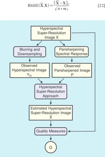
Wald’s protocol for assessing the quality of pansharpening methods [79], depicted in Fig. 2, synthetically generates simu-lated observed images from a reference HS image, and then evaluates the pansharpening methods’ results against that reference image. The protocol consists of the following steps:

◗ _{Given a HS image, X , to be used as reference, a} simulat-ed observsimulat-ed low spatial resolution HS image, YH, is

ob-tained by applying a Gaussian blurring to X , and then downsampling the result by selecting one out of every

d pixels in both the horizontal and vertical directions, where d denotes the downsampling factor.

◗ _{A simulated PAN image, P, is obtained by multiplying} the reference HS image, on the left, by a suitably chosen spectral response vector, P₌r X.T

◗ The pansharpening method to be evaluated is applied to the simulated observations YH and P, yielding the estimated superresolution HS image, .X

t

◗ Finally, the estimated superresolution HS image and the reference one are compared, to obtain quantitative quality measures.

B. QUALITY MEASURES

Several quality measures have been defined in the litera-ture, in order to determine the similarity between esti-mated and reference spectral images. These measures can be generally classified into three categories, depending on whether they attempt to measure the spatial, spectral or global quality of the estimated image. This review is lim-ited to the most widely used quality measures, namely the

cross correlation (CC), which is a spatial measure, the spec-tral angle mapper (SAM), which is a specspec-tral measure, and

the root mean squared error (RMSE) and erreur relative globale

adimensionnelle de synthèse (ERGAS) [85], which are global

measures. Below we provide the formal definitions of these measures operating on the estimated image X Rm n

! m#

W and

on the reference HS image X Rm n

! m# _{. In the definitions,} xj

V and xj denote the jth columns of XW and X,

respec-tively, the matrices ,A B R1 n

! # denote two generic single-band images, and Ai denotes the ith element of A .

1) Cross correlation: The CC, which characterizes the

geo-metric distortion, is defined as

CC _{X X}, _m1 CCS _{X X}i, i , i m 1 = m = m ^W h

/

_W i (19)

where CCS is the cross correlation for a single-band image, defined as CCS _A, , A B A B B j A j n j B j n j A j n j B 1 2 1 2 1 n n n n = - -- -= = = ^ ^ ^ ^ ^ h h h h h

/

where, A 1/n _Aj j n 1

n =^ h/ ₌ is the sample mean of A . The

ideal value of CC is 1.

2) Spectral angle mapper: The SAM, which is a spectral

measure, is defined as SAM X X, _n1 SAM xj,xj , j n 1 = = ^W h

/

_V i (20)

where, given the vectors ,a b_!_Rmm,

( ) , SAM a, a b a, b arccos b ; ;; ; G H = d n (21) a,b aTb

G H = is inner product between a and b, and $ is the ,2 norm. The SAM is a measure of the spectral shape preservation. The optimal value of SAM is 0. The values of SAM reported in our experiments have been obtained by averaging the values obtained for all the image pixels.

3) Root mean squared error: The RMSE measures the ,2 error between the two matrices X and XW

, RMSE X X X X n m F ) = -m ^W h W (22)

FIGURE 2. Flow diagram of the experimental methodology, de-rived from Wald’s protocol (simulated observations), for synthetic and semi-real datasets.

Hyperspectral Super-Resolution Image X Blurring and Downsampling Pansharpening Spectral Response Observed Hyperspectral Image Y_H Observed Pansharpened Image P Hyperspectral Super-Resolution Approach Estimated Hyperspectral Super-Resolution Image Xc Quality Measures Q

(11)

where _X trace _{X X}

F= ^ T h is the Frobenius norm of X . The

ideal value of RMSE is 0.

4) Erreur relative globale adimensionnelle de synthèse:

ER-GAS offers a global indication of the quality of a fused im-age. It is defined as ERGAS( , )_{X X} 100d _m1 RMSE_k k , k m ₂ 1 n = m = m a k W

/

(23)

where d is the ratio between the linear resolutions of the PAN and HS images, defined as

HS linear spatial resolution PAN linear spatial resolution

, d = and RMSEk X X / n , k k F nk

=_ W - i is the sample mean of the kth band of X . The ideal value of ERGAS is 0.

IV. EXPERIMENTAL RESULTS

A. DATASETS

The datasets that were used in the experimental tests were all semi-synthetic, generated according to the Wald’s pro-tocol. In all cases, the spectral bands corresponding to the absorption band of water vapor, and the bands that were too noisy, were removed from the reference image before further processing. Three real-life HS images have been used as ref-erence images for the Wald’s protocol. In the following, we describe the datasets that were generated from these images. Table 2 summarizes their properties. These datasets are ex-pressed in spectral luminance (nearest to the sensor output, without pre-processing) and are correctly registered. 1) Moffett field dataset: This dataset represents a mixed

ur-ban/rural scene. The dimensions of the PAN are 185 # 395 with a spatial resolution of 20m whereas the size of the HS image is 37 # 79 with a spatial resolution of 100m (which means a spatial resolution ratio of 5 be-tween the two images). The HS image has been acquired by the airborne hyperspectral instrument airborne vis-ible infrared image spectrometer (AVIRIS). This instru-ment is characterized by 224 bands covering the spec-tral range 0.4–2.5nm.

2) Camargue dataset: This dataset represents a rural area with different kinds of crops. The dimensions of the PAN image are 500 # 500 with a spatial resolution of 4m whereas the size of the HS image is 100 # 100 with a spatial resolution of 20m, (which means a spatial reso-lution ratio of 5 between the two images). The HS image has been acquired by the airborne hyperspectral instru-ment HyMap (Hyperspectral Mapper) in 2007. The hy-perspectral instrument is characterized by 125 bands covering the spectral range 0.4–2.5nm.

3) Garons dataset: This dataset represents a rural area with a small village. The dimension of the PAN image are 400 #_{400 with a spatial resolution of 4m whereas the size of} the HS image is 80 # 80 with a spatial resolution of 20m, (which means a spatial resolution ratio of 5 between the two images). This dataset has been acquired with the HyMap instrument in 2009.

B. RESULTS AND DISCUSSION

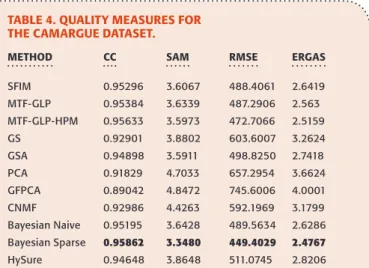
Methods presented in Section II have been applied on the three datasets presented in Section IV-A and analyzed fol-lowing the Wald’s Protocol (Section III-B). Tables 3, 4, 5 report their quantitative evaluations with respect to the quality measures detailed in Section III-B.

Figures 3, 4, and 5 represent the RMSEs per pixel between the image estimated by some methods and the reference

TABLE 2. CHARACTERISTIC OF THE THREE DATASETS. DATASET DIMENSIONS SPATIAL RES N INSTRUMENT Moffett PAN 185 # 395 HS 37 # 79 20m 100m 224 AVIRIS Camargue PAN 500 # 500 HS 100 # 100 4m 20m 125 HyMap Garons PAN 400 # 400 HS 80 # 80 4m 20m 125 HyMap

TABLE 3. QUALITY MEASURES FOR THE MOFFETT FIELD DATASET.

METHOD CC SAM RMSE ERGAS

SFIM 0.96762 7.8313 257.6388 4.6072 MTF-GLP 0.97148 6.9604 253.5582 4.2867 MTF-GLP-HPM 0.96925 7.7301 260.9860 4.5329 GS 0.91722 12.9589 420.5469 7.2204 GSA 0.95304 10.4024 325.1781 5.5938 PCA 0.90664 13.4512 445.1298 7.6215 GFPCA 0.91614 11.3363 404.2979 7.0619 CNMF 0.95633 9.0464 309.9017 5.3469 Bayesian Naive 0.97785 7.1308 220.0310 3.7807 Bayesian Sparse 0.98170 6.6253 200.1856 3.4262 HySure 0.97086 7.3508 253.0972 4.3315

TABLE 4. QUALITY MEASURES FOR THE CAMARGUE DATASET.

(12)

image for the three considered datasets. Note that, for sake of conciseness, some methods have not been considered here but only their improved versions are presented. More specifically, GS has been removed since GSA is an improved version of GS. Indeed, GSA is expected to give better results than GS thanks to its adaptive estimation of the weight for generating the equivalent PAN image from the HS image, which allows the spectral distortion to be reduced. Bayesian naive approach has been also removed since the sparsity-based approach relies on a more complex prior and gives also better results. MTF-GLP and MTF-GLP-HPM yield simi-lar results so only the latter has been considered.

Figures 6 and 7 show extracts of the final result obtained by the considered methods on the Camargue dataset in the visible (R= 704.39nm, G= 557.90nm, B= 454.5nm) and in the SWIR (R= 1216.7nm, G= 1703.2nm, B= 2159.8nm) do-mains, respectively.

Figures 8, 9 and 10 show pixel spectra recovered by the fusion methods, which correspond to 10th, 50th and 90th percentile of RMSE, respectively. Those spectra have been se-lected by choosing GSA as the reference for RMSE value. GSA have been chosen since it is a classical approach that has been widely used in literature and also gives good results. To ensure a reasonable number of figures, only visual results and some spectra of the Camargue dataset has been reported in this article. The results for the two other datasets can be found in the supporting document [86] available online5_{. In}

5_{http://openremotesensing.net}

FIGURE 3. RMSE between the methods’ result and the reference image, per pixel for the Moffett field dataset.

1400 1200 1100 800 RMSE 600 400 200 0 1 # 1 04 2 # 10 4 3 # 10 4 Pixel Number 4 # 10 4 5 # 10 4 6 # 1 04 I_GSA I_SFIM I_PCA I_GFPCA I_CNMF I_Baye Sparse I_Hysure I_MTF_GLP_HPM

FIGURE 4. RMSE between the methods’ result and the reference image, per pixel for the Camargue dataset.

2500 2000 1500 1000 RMSE 500 0 I_GSA I_SFIM I_PCA I_GFPCA I_CNMF I_Baye Sparse I_Hysure I_MTF_GLP_HPM 5.0 # 104 _{1.0 # 10}5 _{1.5 # 10}5 _{2.0 # 10}5 Pixel Number

FIGURE 5. RMSE between the methods’ result and the reference image, per pixel for the Garons dataset.

I_GSA I_SFIM I_PCA I_GFPCA I_CNMF I_Baye Sparse I_Hysure I_MTF_GLP_HPM Pixel Number 2000 3000 4000 1000 RMSE 0 2.0 # 10 4 4.0 # 10 4 6.0 # 10 4 8.0 # 10 4 1.0 # 10 5 1.2 # 10 5 1.4 # 10 5

TABLE 5. QUALITY MEASURES FOR THE GARONS DATASET.

(13)

particular, because of the nature of the Garons dataset (vil-lage with a lot of small buildings) and the chosen ratio of 5, worse results have been obtained than for the two first datasets since a lot of mixing is presented in the HS image.

A visual analysis of the result shows that most of the fusion approaches considered in this paper give good re-sults, excepted two methods: PCA and GFPCA. PCA be-longs to the class of CS methods which are known to be characterized by their high fidelity in rendering the spatial details but their generation of significant spectral distor-tion. This is clearly visible in Figure 6 (f), where significant differences of color can be observed with respect to the reference image, in particular when examining the differ-ent fields. GFPCA here also performs poorly. Compared with PCA, there is less spectral distortion but the included spatial information seems to be not sufficient, since the fused image is significantly blurred. Spatial information provided by PCA is better since the main information of HS image (where the spatial information is contained) is replaced by the high spatial information contained in the

PAN image. When using GFPCA, the guided filter controls the amount of spatial information added to the data, so not all the spatial information may be added to avoid to modify the spectral information too much. For the Mof-fett field dataset, GFPCA performs a little bit better since, in this dataset, there is a lot of large areas. Thus blur is less present whereas, in the Garons dataset, GFPCA performs worse since this image consists of numerous small features, leading to more blurring effects. As a consequence, in this case, GFPCA performs worse than PCA.

To analyze the spectrum in detail, chosen thanks to RMSE percentiles, some additional information about the corresponding pixels are needed. Fig. 9 corresponds to a pixel in the reference image which represents a red build-ing. Since in the HS image this building is mixed with its neighborhood, we do not have the same information be-tween the reference image (“pure” spectrum) and the HS image (“mixed” spectrum). Fig. 8 corresponds to a pixel in a homogeneous field area, no mixing is present and very good results have been obtained for all the methods. For

FIGURE 6. Details of original and fused Camargue dataset HS im-age in the visible domain. (a) reference imim-age, (b) interpolated HS image, (c) SFIM, (d) MTF-GLP-HPM, (e) GSA, (f) PCA, (g) GFPCA, (h) CNMF, (i) Bayesian Sparse, (j) HySure.

(a) (b)

(i) (j)

(c) (d) (e)

(f) (g) (h)

FIGURE 7. Details of original and fused Camargue dataset HS im-age in the SWIR domain. (a) reference imim-age, (b) interpolated HS image, (c) SFIM, (d) MTF-GLP-HPM, (e) GSA, (f) PCA, (g) GFPCA, (h) CNMF, (i) Bayesian Sparse, (j) HySure.

(a) (b)

(i) (j)

(c) (d) (e)

(14)

Fig. 10, the pixel belongs to a small white building not vis-ible in the HS image and spectral mixing is then also pres-ent. More generally, spectra in the HS and reference images differ since some mixing processes occur in the HS image. Thus, the HS pansharpening methods are expected to pro-vide spectra that are more similar to the HS spectra (which contains the available spectral information) than the ref-erence (which has information missing in the HS which should not be found in the result, unless successful unmix-ing has been conducted). However, it is important to note that for Fig. 9, Bayesian methods and HySure successfully

recover spectra that are more similar to the reference spec-trum than the HS specspec-trum.

Table 6 report the computational times required by each HS pansharpening methods on the Camargue data-set those values have been obtained with an Intel Core i5 3230M 2.6 GHz with 8 GB RAM. Based on this table, these methods can be classified as follows:

◗ Methods which do not work well for HS pansharpening: PCA, GS, GFPCA

◗ Methods which work well with a low time of computa-tion (few seconds): GSA, MRA methods, Bayesian Naive ◗ Methods which work well with an average time of

com-putation (around one minute): CNMF

◗ Methods which work well (slightly better) with an impor-tant time of computation (few minutes, depends greatly on the size of the dataset): Bayesian Sparse and HySure.

FIGURE 8. Luminance of the pixel corresponding to the 10th percentile of the RMSE (Camargue dataset).

Spectral Profile 1000 8000 6000 4000 2000 0 500 1000 1500 Wavelength 2000 HS upscale SFIM GSA PCA GFPCA CNMF Baye Sparse Hysure MTF_GLP_HPM Ref . . . .

FIGURE 9. Luminance of the pixel corresponding to the 50th per-centile of the RMSE (Camargue dataset).

Spectral Profile 1.2 # 104 1.0 # 104 8.0 # 103 6.0 # 103 4.0 # 103 2.0 # 103 500 1000 1500 Wavelength 2000 HS upscale SFIM GSA PCA GFPCA CNMF Baye Sparse Hysure MTF_GLP_HPM Ref . . . . Spectral Profile 1.5 # 104 1.0 # 104 5.0 # 103 0 500 1000 1500 Wavelength 2000 HS upscale SFIM GSA PCA GFPCA CNMF Baye Sparse Hysure MTF_GPL_HPM Ref . . . .

FIGURE 10. Luminance of the pixel corresponding to the 90th percentile of the RMSE (Camargue dataset).

TABLE 6. COMPUTATIONAL TIMES OF THE DIFFERENT METHODS (IN SECONDS).

METHOD MOFFETT CAMARGUE GARONS

SFIM 1.26 3.47 2.74 MTF-GLP 1.86 4.26 4.00 MTF-GLP-HPM 1.71 4.25 2.98 GS 4.77 8.29 5.56 GSA 5.52 8.73 5.99 PCA 3.46 8.92 6.09 GFPCA 2.58 8.51 4.36 CNMF 10.98 47.54 23.98 Bayesian Naive 1.31 7.35 3.07 Bayesian Sparse 133.61 485.13 259.44 HySure 140.05 296.27 177.60

(15)

To summarize, the comparison of the different methods performances for RMSE curves and quality measures con-firms than PCA and GFPCA does not provide good results for HS pansharpening (GFPCA is know to perform much better on HS+RGB data). The other methods perform well, with Bayesian approaches having better results. The compu-tational cost of Bayesian approaches depends on the chosen prior, i.e., Bayesian approach with Gaussian naive prior has low cost while the one with sparse prior has higher cost. The favorable fusion per-formance obtained by the Bayesian methods can be ex-plained, in part, by the fact that they rely on a forward modeling of the PAN and HS images and explicitly exploit the spatial and spectral deg-radations applied to the target image. However, these algo-rithms may suffer from per-formance discrepancies when the parameters of these degra-dations (i.e., spatial blurring kernel, sensor spectral response) are not perfectly known. In particular, when these parameters are fully unknown and need to be fixed, they can be estimated jointly with the fused image, as in [53], or estimated from the MS and HS images in

a preprocessing step, following the strategies in [78] or [35]. CS methods are fast to compute and easy to implement. They provide good spatial results but poor spectral results with sig-nificant spectral distortions, in particular when considering PCA and GS. GSA provides better results than the two other methods thanks to its adaptive weight estimation reducing the spectral distortion of the equivalent PAN image cre-ated from the HS image. MRA methods are fast, MTF-based methods give better results than SFIM and perform as well as the most competitive algorithms with higher computational complexity. SFIM does not perform as well than the other MRA methods since it uses a box filter which should give less good result. In our experimentations, results from SFIM are not so different from those obtained with the MTF-based methods. This may come from the fact that semi-synthetic datasets are used so MTF may not be fully used to its poten-tial. Table 7 reports these pro and cons associated with each HS pansharpening method.

Finally, note that, in our experimentations, no registra-tion error and temporal misalignment have been considered, which suggests that the robustness of the different methods has not been fully analyzed. When such problems may oc-cur, CS and MRA methods may perform better thanks to their great robustness. In particular, CS methods are robust against misregistration error and aliasing, whereas MRA ap-proaches are robust against aliasing and temporal misalign-ment. It is also worthy to note that the quality of a fusion method should also be related to a specific application (such

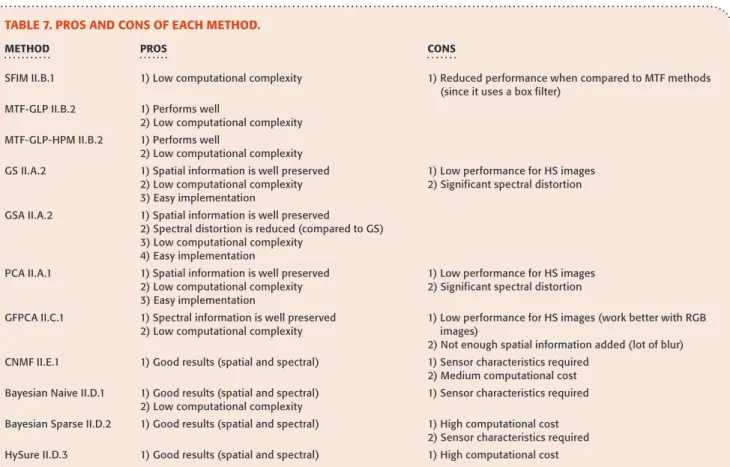
TABLE 7. PROS AND CONS OF EACH METHOD.

METHOD PROS CONS

SFIM II.B.1 1) Low computational complexity 1) Reduced performance when compared to MTF methods (since it uses a box filter)

MTF-GLP II.B.2 1) Performs well

2) Low computational complexity MTF-GLP-HPM II.B.2 1) Performs well

2) Low computational complexity GS II.A.2 1) Spatial information is well preserved

2) Low computational complexity 3) Easy implementation

1) Low performance for HS images 2) Significant spectral distortion GSA II.A.2 1) Spatial information is well preserved

2) Spectral distortion is reduced (compared to GS) 3) Low computational complexity

4) Easy implementation

PCA II.A.1 1) Spatial information is well preserved 2) Low computational complexity 3) Easy implementation

1) Low performance for HS images 2) Significant spectral distortion GFPCA II.C.1 1) Spectral information is well preserved

2) Low computational complexity

1) Low performance for HS images (work better with RGB images)

2) Not enough spatial information added (lot of blur) CNMF II.E.1 1) Good results (spatial and spectral) 1) Sensor characteristics required

2) Medium computational cost Bayesian Naive II.D.1 1) Good results (spatial and spectral)

2) Low computational complexity

1) Sensor characteristics required Bayesian Sparse II.D.2 1) Good results (spatial and spectral) 1) High computational cost

2) Sensor characteristics required HySure II.D.3 1) Good results (spatial and spectral) 1) High computational cost FOLLOWING WALD’S

PROTOCOL, THE EVALUATION INCLUDES QUALITATIVE VISUAL ASSESSMENT, AS WELL AS QUANTITATIVE EVALUATION WITH A NUMBER OF CRITERIA MEASURING SPATIAL AND SPECTRAL DISTORTIONS.