O
pen
A
rchive
T
OULOUSE
A
rchive
O
uverte (
OATAO
)
OATAO is an open access repository that collects the work of Toulouse researchers and
makes it freely available over the web where possible.
This is an author-deposited version published in :
http://oatao.univ-toulouse.fr/
Eprints ID : 17092
The contribution was presented at XX :
https://signalprocessingsociety.org/blog/camsap-2015
To cite this version :
Costa, Facundo and Batatia, Hadj and Oberlin, Thomas and
Tourneret, Jean-Yves EEG source localization based on a structured sparsity
prior and a partially collapsed Gibbs sampler. (2015) In: 6th IEEE International
Workshop on Computational Advances in Multi-Sensor Adaptive Processing
(CAMSAP 2015), 13 December 2015 - 16 December 2015 (Cancun, Mexico).
Any correspondence concerning this service should be sent to the repository
administrator:
[email protected]
EEG Source Localization Based on a Structured
Sparsity Prior and a Partially Collapsed Gibbs
Sampler
Facundo Costa, Hadj Batatia, Thomas Oberlin, Jean-Yves Tourneret
University of Toulouse, INP/ENSEEIHT - IRIT, 2 rue Charles Camichel, BP 7122, 31071 Toulouse Cedex 7, France
Abstract—In this paper, we propose a hierarchical Bayesian model approximating the ℓ20 mixed-norm regularization by a
multivariate Bernoulli Laplace prior to solve the EEG inverse problem by promoting spatial structured sparsity. The posterior distribution of this model is too complex to derive closed-form expressions of the standard Bayesian estimators. An MCMC method is proposed to sample this posterior and estimate the model parameters from the generated samples. The algorithm is based on a partially collapsed Gibbs sampler and a dual dipole random shift proposal for the non-zero positions. The brain activity and all other model parameters are jointly estimated in a completely unsupervised framework. The results obtained on synthetic data with controlled ground truth show the good performance of the proposed method when compared to the ℓ21
approach in different scenarios, and its capacity to estimate point-like source activity.
Index Terms—EEG, MCMC, inverse problem, source localiza-tion, structured-sparsity, hierarchical Bayesian model, ℓ20-norm
regularization
I. INTRODUCTION
EEG source localization is an ill-posed inverse problem [1] that continues to attract a significant amount of interest in the signal and image processing literature. The problem is classically addressed using some regularization that enforces realistic properties on the solution. Among the proposed regu-larizations, the ℓ0pseudo-norm is known to estimate correctly sparse focal brain activity [2]. Unfortunately, the minimization of the ℓ0 pseudo-norm is intractable. Thus it is usually approximated by the convex ℓ1norm that can be handled more easily using classical optimization techniques [3] but does not provide the same solution [2]. In a previous work, we have proposed to combine them in a Bayesian framework providing good results [4]. However this method, as the ℓ0and ℓ1norms, considers each time sample independently which can lead to unrealistic solutions [5]. It has been shown that structured sparsity can provide better results by exploiting the temporal dimension of the data [6]. Structured sparsity can be enforced for EEG source localization using mixed-norms such as the ℓ21 norm [5] (also known as group-lasso), which constrains all the time samples of a dipole to be either completely active or inactive during the time period. As an alternative to the ℓ21 norm, we introduce a new hierarchical Bayesian model based on a multivariate Bernoulli Laplacian prior on the dipole activity. This paper will show that the proposed prior allows sparser solutions to be obtained. Since the posterior associated with this prior is intractable, a Markov chain Monte
Carlo sampling technique is used to draw samples of the unknown parameters asymptotically distributed according to this posterior. A dual dipole random shift proposal is also added in order to improve convergence. The generated samples are then used to estimate both the brain activity and the model parameters and hyperparameters in a completely unsupervised framework.
The paper is organized as follows: Section II introduces the proposed Bayesian model. Section III presents the partially collapsed Gibbs sampler that can generate samples asymp-totically distributed according to the posterior of this model. Results obtained with synthetic data are presented in Section IV. Section V concludes the paper.
II. PROPOSED METHOD
We consider a distributed-source model that has a fixed number (N) of dipoles on the cortical surface whose orien-tations are supposed orthogonal to the cortex [1]:
Y = HX + E (1)
where X∈ RN ×T contains the amplitudes of the N dipoles for the corresponding T time samples, Y ∈ RM ×T contains the measurements of the M electrodes for these T time samples, H∈ RM ×N models the propagation of the electro-magnetic field from the sources to the sensors and E∈ RM ×T is a noise term. The EEG source localization problem consists of estimating the matrix X from the measurements Y , which we propose to solve with the following Bayesian model. A. Likelihood
It is very classical in the literature to consider an additive white Gaussian noise with a constant variance σ2
n for the T considered time instants [1]. Note that when this assumption does not hold, it is possible to estimate the noise covariance matrix from the data and to whiten the measurements in a pre-processing stage [5]. This assumption leads to the likelihood
f(Y |θ) = T ! t=1 N"yt # # #Hx t,σ2 nIM $ (2)
where IM is the identity matrix of size M , θ= {X, σ2 n} and mj denotes the j-th column of matrix M .
B. Priors
Dipole amplitudes X
The weighted ℓ20 pseudo norm of a matrix X with rows x1, ..., xN is defined by
||X||20= #{i :√vi||xi||2#= 0} (3) where #S is the cardinal of the set S and vi = ||hi||2 (hi being the i-th column of the operator H) is a weight used to compensate for the depth-weighting effect as explained in [1, 3]. We propose to approximate the ℓ20mixed norm using a multivariate Bernoulli Laplace prior for each row xi of X. More precisely, we consider the following prior
f(xi|zi, a,σ2 n) ∝ % δ(xi) if zi= 0 exp"−&via σn2||xi||2 $ if zi= 1 (4) where a is a hyperparameter that controls the amplitudes of the non-zero rows of X and z∈ {0, 1}N is a vector indicating which rows of X are non-zero. The elements of z are assigned a Bernoulli prior with parameter ω∈ [0, 1]
zi|ω ∼ B (zi|ω) . (5)
Note that the prior of xi defined in (4) contains two different parts: the Dirac delta function δ(.) that promotes sparsity by ensuring absence of activity and the multivariate Laplace distribution that adjusts the amplitudes of the non-zero rows. Setting ω = 0 reduces to X = 0 whereas ω = 1 corre-sponds to the ℓ21-mixed norm regularization introduced in the Bayesian formulation of the group-lasso. To be able to sample efficently from the posterior distribution of the model parameters, it is interesting to introduce a latent variable τ2 i for each row xi as in [7]. More precisely, the joint prior distribution of(τ2
i, xi) can be defined as f(τ2 i|a) =G " τ2 i # # # T + 1 2 , via 2 $ (6) f(xi|zi,τ2 i,σ 2 n) = % δ(xi) if zi= 0 N"xi # # #0,σ 2 nτ 2 iIT $ if zi= 1 (7) where G and N denote the gamma and normal distributions. Indeed, the prior distribution specified above is such that the marginal distribution of xi is (4) [7].
Noise varianceσ2 n
The noise variance σ2
n is assigned a Jeffrey’s prior f(σ2
n) ∝ σ12 n
1R+(σn)2 (8)
where 1R+(ξ) = 1 if ξ ∈ R+ and 0 otherwise. Motivations
for using this prior can be found in [8].
C. Hyperparameter priors
In the ℓ21norm based approach, the regularization parame-ter makes a compromise between the sparsity of the solution and the fidelity to the measurements. In the proposed Bayesian model, this compromise is adjusted by two hyperparameters: (1) ω that determines the proportion of the rows of X that are zero and (2) a that controls the amplitudes of the non-zero rows of X. We will denote the hyperparameter vector by φ= {ω, a}. To make our algorithm capable of estimating the values of ω and a from the data, we need to assign priors to these hyperparameters (usually called hyperpriors).
A conjugate gamma prior is chosen for a for simplicity f(a|α, β) = G"a # # #α, β $ (9) with α= β = 1. This choice of (α, β) corresponds to a vague hyperprior for a.
A non-informative uniform prior on [0, 1] is used for ω f(ω) = U (ω|0, 1) (10) also reflecting the absence of knowledge for this parameter. D. Posterior distribution
Using the priors and hyperpriors defined in Section II, the posterior distribution of the proposed Bayesian model can be derived as follows
f(θ, z, τ2, φ
|Y ) ∝ f(Y |θ)f(θ|z, τ2)f (z, τ2|φ)f (φ) (11) where f(Y |θ) has been defined in (2) and
f(θ|z, τ2 ) ∝ f(σ2 n) N ! i=1 f(xi|zi,τi2,σ 2 n) f(z, τ2|φ) = N ! i=1 f(zi|ω)f (τ2 i|a) f(φ) = f (a|α, β)f (ω).
III. APARTIALLY COLLAPSEDGIBBS SAMPLER
The Bayesian estimators of the unknown model parameters σ2
n, X, z, a, τ
2,ω are clearly difficult to express in closed form using (11). Thus, we propose to draw samples from the posterior distribution (11) and use these samples to estimate the model parameters and hyperparameters using a partially collapsed Gibbs sampler which samples the variables zi and xi jointly. The corresponding conditional distributions are detailed in the following sections.
A. Conditional distributions
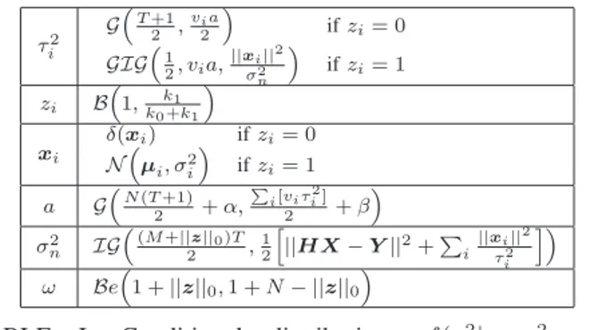
The conditional distributions of the different parameters and hyperparameters are provided in Table I, whereG, GIG, N , B, IG and Be stand for the gamma, generalized inverse Gaus-sian, normal, Bernoulli, inverse gamma and beta distributions respectively (for the definition of the GIG distribution, see [7]).
τ2 i G!T+1 2 , via 2 " if zi= 0 GIG!1 2, via,||xi|| 2 σ2n " if zi= 1 zi B ! 1, k1 k0+k1 " xi δ(xi) if zi= 0 N!µi,σi2 " if zi= 1 a G!N(T +1)2 + α,!i[viτi2] 2 + β " σ2 n IG !(M +||z||0)T 2 ,12 # ||HX − Y ||2+$ i ||xi||2 τ2 i %" ω Be!1 + ||z||0,1 + N − ||z||0 "
TABLE I: Conditional distributions f(τ2 i|xi,σ 2 n, a, zi), f(zi|Y , X−i,σ 2 n,τ 2 i,ω), f (xi|zi, Y , X−i,σ 2 n,τ 2 i), f (a|τ 2), f(σ2 n|Y , X, τ 2, z) and f (ω, z).
We denote by X−i the matrix X with its i-th row set to zero and µi= σ 2 ih iT (Y − HX−i) σ2 n ,σ2 i = σ2 nτi2 1 + τ2 ihiThi k0= 1 − ω, k1= ω ' σ2 nτi2 σ2 i (−T 2 exp"||µi|| 2 2σ2 i $ . B. Dual dipole random shift proposal
In practice, the Gibbs sampler can get trapped in local maxima of the target distribution, especially when the indicator variables zi have to be sampled. This problem has been reported in several works such as [9] and has been observed for the proposed partially collapsed Gibbs sampler. To solve this problem, after each sampling iteration, a new value of z can be proposed in order to escape from a possible local maximum. This value is accepted or rejected using the Metropolis-Hastings acceptance ratio to keep the same target distribution. In this work, we have implemented dual dipole random shift proposals which consist of moving up to two indicators within their neighborhood, which is defined as follows
neighγ(i)!)j#= i # # # |corr(h i, hj )| ≥ γ* (12) where corr(hi, hj) is the correlation between the two column vectors and γ ∈ [0, 1] tunes the neighborhood size (γ = 0 corresponds to a neighborhood containing all the dipoles and γ= 1 corresponds to an empty neighborhood). In our exper-iments, we have used γ= 0.8, adjusted by cross validation.
IV. EXPERIMENTAL VALIDATION
A comparison with the ℓ21approach has been done consid-ering the Stok three-shell head model with M = 41 electrodes and N = 212 dipoles. Synthetic damped sinusoidal excitations with frequencies between 5 and 20Hz were assigned to the active dipoles dipoles. These excitations are 500ms long (a period in which the dipole activity is known to be stationary) and sampled at200Hz, resulting in T = 100. The regularization parameter of the weighted ℓ21norm was set according to the uncertainty principle.
(a) Ground truth
(b) Proposed method
(c) Weighted ℓ21-norm
Fig. 1: Typical brain activity localization (SNR =−3dB). Two different kind of simulations were run, the first one has a fixed amount of active dipoles in the ground truth and a variable level of SNR whereas the second one presents a fixed level of SNR with a variable amount of active dipoles.
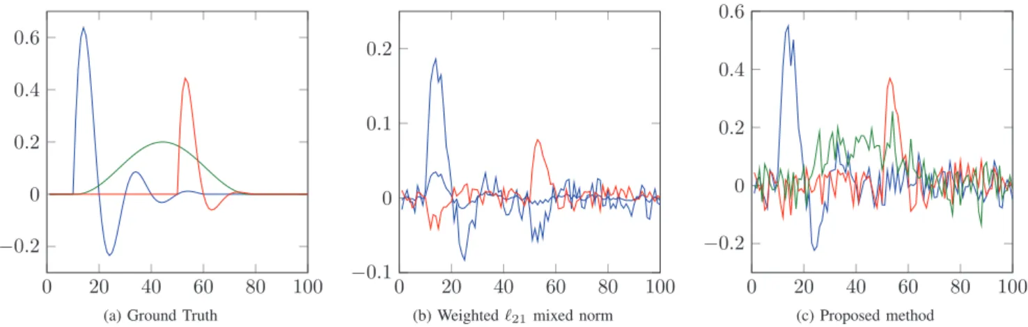
For the first kind of simulations three dipoles were active in the ground truth. For high SNR values (20dB or more), both methods are able to correctly detect the dipole locations and estimate their activation waveforms. However, as the SNR decreases, the proposed method outperforms the approach based on the ℓ21norm. A representative example is illustrated in Figs. 1 and 2. As we can see in this particular case, the proposed algorithm manages to recover correctly the three activations while concentrating each of the activations in only one dipole. In comparison, the ℓ21 norm only recovers two activations and spreads some of the activity between neighboring dipoles. One can also see that the waveforms recovered by the proposed method are much closer to the original excitations than those obtained with the ℓ21 norm (note the presence of a bias with the latter). This result can be explained by the fact that the ℓ1 norm tends to overpenalize large amplitudes whereas the proposed prior penalizes all non-zero coefficients equally.
For the second kind of simulations, the SNR was set to 30dB while the amount of active dipoles in the ground truth (denoted by P ) was varied from 1 to 7. Fifty different active dipole localizations were used for each value of P . After each simulation run, the P dipoles with highest estimated activity were considered to be active. The recovery rate (defined as the probability of detecting an active dipole in its correct location) for both methods is shown in Table II. The proposed method is able to detect up to 5 active dipoles with a near perfect recovery rate while the performance of the ℓ21norm method
0 20 40 60 80 100 −0.2 0 0.2 0.4 0.6
(a) Ground Truth
0 20 40 60 80 100
−0.1 0 0.1 0.2
(b) Weighted ℓ21mixed norm
0 20 40 60 80 100 −0.2 0 0.2 0.4 0.6 (c) Proposed method
Fig. 2: Ground truth and typical estimated time waveforms with SNR = -3dB.
starts decreasing at P = 3.
It is important to note that the price to pay with the proposed method is its computational complexity. One simulation of the previous examples was processed in 6 seconds with a modern Xeon CPU E3-1240 @ 3.4GHz processor (using a Matlab implementation with MEX files written in C) against 104 milliseconds for the ℓ21mixed norm. However, also note that the ℓ21 norm approach requires running the algorithm multiple times to adjust the regularization parameter by cross-validation.
P 1 - 2 3 4 5 6 7
PM 100% 100% 100% 98.8% 84.0% 65.1%
ℓ21 100% 97.3% 93.5% 78.8% 61.7% 49.1%
TABLE II: Recovery rate as a function of P for the proposed method and the weighted ℓ21norm (computed with50 Monte Carlo runs).
V. CONCLUSION
This paper introduced a new hierarchical Bayesian model for EEG source localization promoting structured sparsity using a multivariate Bernoulli Laplacian prior. A partially collapsed Gibbs sampler was developed to draw samples from its posterior distribution. A specific Metropolis-Hastings move (called dual dipole random shift) was also introduced in order to speed up the algorithm convergence. The generated samples were used to estimate the source activity and the model hyperparameters jointly in an unsupervised framework. The resulting algorithm was compared to the ℓ21 mixed norm regularization showing promising results for synthetic data composed by point-like source activations. More precisely, the proposed method showed better detection results and a better recovery of the activation waveforms for small SNRs, while avoiding the amplitude underestimation observed with the ℓ21approach. In addition, the proposed method presented a better recovery rate for different amounts of active dipoles. The method is currently being applied to real data and is already showing promising results which will be published in
the near future. Future work will try to generalize the method to practical cases whereH is only partially known.
REFERENCES
[1] R. Grech, T. Cassar, J. Muscat, K. P. Camilleri, S. G. Fabri, M. Zervakis, P. Xanthopoulos, V. Sakkalis, and B. Vanrumste, “Review on solving the inverse problem in EEG source analysis,” J. Neuroeng. Rehabil., vol. 4, pp. 5–25, 2008.
[2] E. J. Candes, “The restricted isometry property and its implications for compressed sensing,” C. R. l’Acad´emie des Sciences, vol. 346, no. 9, pp. 589–592, 2008. [3] K. Uutela, M. H¨am¨al¨ainen, and E. Somersalo,
“Visual-ization of magnetoencephalographic data using minimum current estimates,” NeuroImage, vol. 10, no. 2, pp. 173– 180, 1999.
[4] F. Costa, H. Batatia, L. Chaari, and J.-Y. Tourneret, “Sparse EEG Source Localization using Bernoulli Laplacian Priors,” IEEE Trans. Biomed. Eng., doi: 10.1109/TBME.2015.2450015, to be published.
[5] A. Gramfort, M. Kowalski, and M. H¨am¨al¨ainen, “Mixed-norm estimates for the M/EEG inverse problem using accelerated gradient methods,” Phys. Med. Biol., vol. 57, no. 7, p. 1937, 2012.
[6] J. Huang and T. Zhang, “The benefit of group sparsity,” Ann. Statist., vol. 38, no. 4, pp. 1978–2004, Aug. 2010. [7] S. Raman, T. J. Fuchs, P. J. Wild, E. Dahl, and V. Roth,
“The Bayesian group-lasso for analyzing contingency ta-bles,” in Proc. 26th ACM Annu. Int. Conf. Mach. Learn. (ICML), Montreal, Quebec, Jun. 2009.
[8] G. Casella and C. P. Robert, Monte Carlo Statistical Methods. New York: Springer-Verlag, 1999.
[9] S. Bourguignon and H. Carfantan, “Bernoulli-Gaussian spectral analysis of unevenly spaced astrophysical data,” in Proc. IEEE Workshop on Stat. Signal Processing (SSP), Bordeaux, France, Jul. 2005.