O
pen
A
rchive
T
OULOUSE
A
rchive
O
uverte (
OATAO
)
OATAO is an open access repository that collects the work of Toulouse researchers and
makes it freely available over the web where possible.
This is an author-deposited version published in :
http://oatao.univ-toulouse.fr/
Eprints ID : 15292
To link to this article :
URL :
http://dx.doi.org/10.1109/RCIS.2015.7128908
To cite this version :
Berro, Alain and Megdiche-Bousarsar, Imen and Teste, Olivier
Holistic Statistical Open Data Integration Based On Integer Linear
Programming. (2015) In: IEEE 9th International Conference on
Research Challenges in Information Science (RCIS 2015), 13 May
2015 - 15 May 2015 (Athens, Greece)
Any correspondence concerning this service should be sent to the repository
administrator:
[email protected]
Holistic Statistical Open Data Integration Based On
Integer Linear Programming
Alain Berro, Imen Megdiche, Olivier Teste
IRIT UMR 5505, University of Toulouse, CNRS, INPT,UPS, UT1, UT2J
31062 TOULOUSE Cedex 9, France {Alain.Berro, Imen.Megdiche, Olivier.Teste}@irit.fr
Abstract—Integrating several Statistical Open Data (SOD) tables is a very promising issue. Various analysis scenarios are hidden behind these statistical data, which makes it important to have a holistic view of them. However, as these data are scattered in several tables, it is a slow and costly process to use existing pairwise schema matching approaches to integrate several schemas of the tables. Hence, we need automatic tools that rapidly converge to a holistic integrated view of data and give a good matching quality. In order to accomplish this objective, we propose a new 0-1 linear program, which automatically resolves the problem of holistic OD integration. It performs global optimal solutions maximizing the profit of similarities between OD graphs. The program encompasses different constraints related to graph structures and matching setup, in particular 1:1 matching. It is solved using a standard solver (CPLEX) and experiments show that it can handle several input graphs and good matching quality compared to existing tools.
Keywords—Schema Matching, Linear Programming, Statistical Open Data
I. INTRODUCTION
Crossing and analysing Statistical Open Data (SOD) in data warehouses is a promising issue. However, the characteristics of SOD make them unaffordable with traditional ETL (Extract-Transform-Load) processes. Indeed, an important part1of SOD holds into spreadsheets disposing structurally and semantically heterogeneous tables. Moreover, these sources are scattered across multiple providers and even in the same provider, which hampers their integration.
To cope with these issues, we have proposed a graph-based ETL approach composed of three steps which adapt the extract, transform and load traditional ETL steps. The first step extracts, annotates and transforms the SOD tables into a unified graph representation [1]. The second one gives a solution to the automatic holistic data integration problem through the Integer Linear Programming (ILP) technique. The third step focuses on an incremental multidimensional schema definition from the integrated graphs.
In this paper, we focus on the second phase of our ETL processes by resolving the problem of schema matching. According to [2], transformations (in ETL) can be defined from the correspondences between schema elements resolved
1http://fr.slideshare.net/cvincey/opendata-benchmark-fr-vs-uk-vs-us.
The percentage of flat OD sources is 82% in France providers, 65% in United States providers and 66% in United Kingdom providers.
by a matching task. Furthermore, the number of input schemas declines the schema matching problem into pairwise (2 input schemas) and holistic (several input schemas) problems [2]. Our proposition falls within the holistic schema matching approaches. It consists of an integer linear program reducible to the weighted graph matching problem and extends this latter with different constraints on graph structures and matching setup.
A. An overview of the Graph-Based ETL Approach
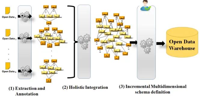
Our approach aims to offer users an easy and repetitive way to reuse SOD in different analysis scenarios by bringing automatic solutions in the ETL processes. Our processes are based on the idea of manipulating graphs. Different reasons motivated our choice: (i) graph data models [3] have gained attention from different research communities in previous years; (ii) graphs are flexible as they hold objects and relation-ships varying from the most generic and simple to the more specific and complex. Our approach [4] takes as input flat SOD spreadsheets and generates as output multidimensional schemas [5]. It involves three main steps as depicted in Fig.1: • ”Extraction and Annotation”: the first step takes as input flat SOD spreadsheets and provides unified instance-schema graphs. In [1], we have proposed a solution to perform this step. The idea consists of exploiting and enriching table anatomies in order to automatically define the schema of tables. The spreadsheets contain tables which are composed of: (i) numerical data (the statistics or numerical values in tables) and (ii) structural data (the text surrounding tables in rows or columns). We have encoded the cell types into matrices, in which we apply several algorithms to extract the different blocks composing a table. These blocks are annotated according to three overlapping types. For more details refer to [1]. Two classification approaches have been applied in order to transform structural data into hierarchies. The extracted and annotated parts are transformed into a unified instance-schema graph representation. The latter is stored in a staging area.
• ”Holistic Integration”: the second step takes as input structural parts of several graphs and generates as out-put an integrated graph and the underlying matchings. The integrated graph is composed of collapsed and
Fig. 1. A Graph-Based ETL Approach
simple vertices connected by simple edges. Collapsed vertices reference groups of matched vertices. Non-matched ones remain simple vertices. We propose an integer linear program to perform an automatic and optimal holistic integration. Users can validate and/or adjust the proposed solution. It maximizes semantic and syntactic similarity between the labels of the vertices of all inputted graphs. It also resolves conflicting situations by ensuring strict hierarchies [6] and preserving logical edges’ directions.
• ”Incremental Multidimensional Schema Definition” : the final step takes as input an integrated graph and generates a multidimensional schema. An interactive process is established between users’ actions and system:
◦ users’ actions consist of identifying multidi-mensional components such as dimensions, parameters, hierarchies, facts and measures. These actions are defined in increment. Users should begin by identifying the dimensions and their components (hierarchies and parameters). Then, they define the fact and its measures forming a multidimensional schema.
◦ the system interacts with users’ actions, first, by transforming the integrated graph into a multidimensional schema. Next, it generates a script describing the multidimensional schema, from which the data warehouse is populated with information.
B. Motivating Example
An agricultural company in England aims to launch a new project on cereal production. The company is interested in analysing England cereal production activity in the previous years. The study consists of reusing SOD from one or different providers. Some data were collected from the World Bank provider. This reference shares more than 1,000 statistical
indicators by topic, year and country. For the ”Agriculture & Rural Development”2 topic, the company noticed some relevant indicators, like cereal yield or crop production. Hence, the spreadsheets3corresponding to these indicators for the UK have been selected for the analysis study. Since the World Bank statistics are aggregated, the company collected other sources to deepen the study. They proposed to use the SOD from the UK governmental provider4. The latter provides several detailed sources for cereal production by cereal type, farm size, type, etc. Our approach perfectly meets this case study for the following reason. For several heterogeneous SOD sources, a rapid and automatic integration is advantageous to this company. They will conserve resources and time by avoiding a large amount of manual work.
This example will be used as a running example in the remainder of this paper.
In the next section, we discuss our holistic integration proposal to the existing work of literature. The remainder of this paper is organized as follows. In Section II, we study some relevant related works. In Section III, we present our holistic integration approach applied on SOD graphs. Section IV will be devoted to comparative experiments according to other approaches. We conclude this work in Section V.
II. RELATEDWORKS
Schema matching problem is among the most studied problems as it represents a key task in several application fields including data integration. The schema matching task consists of identifying semantic correspondences (mappings or alignments) between data models such as database schemas, XML schemas and ontologies [7]. The general workflow for schema matching [7] is composed of a pre-processing step, an execution step for one or several matchers, a combination of
2http://data.worldbank.org/indicator
3http://data.worldbank.org/country/united-kingdom
4
matcher(s) results and finally a selection of correspondences. We have observed that one or several steps in this workflow are reduced to a combinatorial optimisation problem. The latter criteria and further ones have been summarized in Table I to compare our approach, named LP4HM, with some related works. The criteria we have chosen are: (1) the type of approaches, namely pairwise or holistic, (2) the internal model representation, (3) the application to a domain, (4) the reduction to a known combinatorial optimisation problem, its complexity and in which step the reduction is noticed, (5) the dependence of a threshold and (6) the elemental or structural techniques. We refer to [8] for the classification of these techniques. We will first describe some related works, then we will discuss the main differences and similarities of our approach compared to these works.
Holistic Approaches: These approaches generate cor-respondences for several input schemas. In this paragraph, we describe DCM [9], HSM [10], PORSCHE [11] and PLASMA [12] holistic propositions. DCM and HSM are applied for matching web query interfaces. Their schemas are a list of attributes extracted from the web query interfaces. The Dual Correlation Mining (DCM) algorithm computes groups of positively correlated attributes (co-occur in the same query interface). Then it discovers matching by computing negative correlation (not co-occur in the same query interface) among groups of attributes. The selection of the final correspondences is done by a greedy selection using threshold, ranking and scor-ing functions. The Holistic Schema Matchscor-ing (HSM) is similar to the DCM approach according to the co-occurence idea. The HSM algorithm computes between every two attributes of all the schemas: (i) a matching score for the attributes that are frequently co-present and (ii) a grouping score for the attributes that are rarely co-present. The selection of the final correspon-dences is done by an iterative algorithm using grouping scores and thresholds. PORSCHE and PLASMA holistic approaches handle tree XML or XSD schemas. PORSCHE focuses on Book domain and PLASMA on E-Business domain. Both approaches use the clustering technique. PORSCHE uses the tree mining technique in order to construct clusters of similar elements. Element-level similarity is based on a local thesaurus and abbreviation. An incremental algorithm is applied to compute final correspondences using node ranks representing the node contexts. PLASMA applies, holistically, the algorithm Dryade [13] to extract the frequent sub-trees, then they com-pute string-based similarities between the elements of these sub-trees in order to keep the most relevant ones. To compute structural similarities, they apply an enhanced version of the EXSMAL [14] algorithm between all pairs of frequent sub-trees independently. Different thresholds and weighting are used in PLASMA to combine and select correspondences.
Pairwise Approaches: These approaches generate cor-respondences for two input schemas. In this paragraph, we describe COMA++ [15], Similarity Flooding [16], BMatch [17], CODI [18] and OLA [19] pairwise approaches. COMA++ is a generic pairwise matcher applied for ontologies, XML schema and relational databases. It transforms input sources into a directed acyclic graph. Seventeen elemental and struc-tural level matchers are executed in parallel. The strucstruc-tural matchers focus on computing structural similarities between children, paths and leaves. The Similarity Flooding (SF) pair-wise approach converts input sources into labelled graphs. The
structural-level matcher of SF takes as input the similarities of string-based element level matchers, then it propagates similarities between neighbourhood nodes until a fixed point computation. One among the filters of SF is based on the stable marriage problem that returns a local optimal solution [20]. The BMatch [17] pairwise approach handles tree schemas. It combines two element-level matchers and a structural-level matcher. This latter measures structural similarities based on the context of nodes and uses a b-tree to improve the matching performance.
The pairwise matcher CODI implements the probabilistic Markov logical framework presented in [21] for ontology matching. This framework transforms the matching problem to a maximum-a-posteriori (MAP) optimisation problem that is equivalent to Max-Sat problem (NP-hard). The MAP problem encompasses cardinality and coherence constraints, as well as stability constraints. It aims to maximize the probability of the potential alignments. This framework is generic since it considers classes, properties and individuals in the ontologies. It is solved through an Integer Linear Program (ILP) but the authors of [21] omit the details of their program. The pairwise approach OLA aims to match ontologies. It uses labelled graphs as internal representation. The resolution of this problem is carried out by an iterative algorithm. Indeed, the OLA algorithm takes as input the similarities resulting from the element-level matcher, then computes iteratively structural similarities for properties and elements. It does it through a set of equations. The resolution finishes when a fixed point is attempted. The filtering step of OLA is reduced to a weighted bipartite graph matching problem.
Discussion: Unlike the other approaches, only CODI and LP4HM can resolve, in the same time, the structural matching phase without additional structural similarity compu-tation and the correspondences extraction phase. All the other approaches compute an additional structural similarity through their structural-level matcher. The integer linear program of LP4HM is reduced, in pairwise scenarios, to the maximum weight bipartite graph matching problem (MWBG), just like what OLA has done for the filtering phase. The complexity of the maximum-weighted bipartite graph matching problem with an integer linear program is polynomial [22], even with the simplex algorithm [22] [23]. For holistic scenarios, LP4HM is reduced to the maximum weighted non-bipartite graph matching problem [22] which can also be solved in polynomial time by some algorithm like the Edmonds’ algorithm [24]. Unlike CODI, whose pairwise approach is reduced to an NP-Hard problem, our proposed solution extends a polynomial problem in both pairwise and holistic versions.
Another point of discussion is the optimality of the pro-posed solution. In combinatorial optimisation, we distinguish local and global optimal solutions. A local optimum is a solution better than all neighbourhood solutions whilst a global optimum is the best solution among all the possible solutions of a problem. In the same conditions, local optimum is lower than or equal to global optimum. For the pairwise matching approaches SF and OLA, the authors of [20] emphasizes that the stable marriage filter of SF returns a local optimal solution and the maximum weight matching filter of OLA returns a global optimal solution. They also show through the example
TABLE I. ASYNTHETIC COMPARISON OFLP4HMWITH SOME RELATED WORKS
Approach Type Internal
Model
Domain App.
Combinatorial Optimisation Reduction Dep. Thresh-old
Matching techniques
Problem Complexity Used In Element-level Structural-level
DCM holistic list of
at-tributes
Yes - - - Yes linguistic based
-HSM holistic list of
at-tributes
Yes - - - Yes linguistic based
-PORSCHE holistic tree Yes - - - No linguistic-based tree mining
PLASMA holistic tree Yes - - - Yes string-based Exsmal algorithm
COMA++ pairwise directed acyclic graphs No - - - Yes string, constraint, language, linguistic based matching subtrees, children, leaf and path similarities Similarity Flooding pairwise labelled graphs No Stable Marriage
polynomial filtering Yes string-based structural
similarity propagation until fixed point computation
BMatch pairwise tree No - - - Yes string-based Btree
CODI pairwise labelled
graph
No Max-SAT NP-hard structural
matcher and filtering
Yes string-based integer linear con-straints
OLA pairwise labelled
graph
No Maximum
weighted graph matching
polynomial filtering Yes string constraint, linguistic based similarity equation fixed point LP4HM holistic directed acyclic graphs No Maximum weighted graph matching polynomial structural matcher, filtering
No string and lin-guistic based
integer linear con-straints
on pages 132-136 ([20]) that the local optimum of SF is lower than the global optimum of OLA for pairwise matching in the same conditions. Since our approach is reducible to finding a maximum weight matching (in bipartite graph in case of pairwise matching or in non-bipartite graph in case of holistic matching), our approach returns also globally optimal solutions representing the best assignments over all possible solutions maximizing the sum of the weights.
We note some differences between OLA and our approach: OLA uses an iterative algorithm to compute structural similar-ities then it applies the principle of the MWBG in filtering; LP4HM extends the integer linear program of the MWBG with structural constraints without additional structural similarity computation. OLA focuses on ontologies while LP4HM fo-cuses on hierarchical trees to resolve SOD integration problem in multidimensional data warehouses. LP4HM can be applied for taxonomic ontologies but not for the other types of ontolo-gies.
The use of the holistic approaches DCM and HSM is limited to a list of attributes, so they are not applicable on structured schemas namely hierarchical graphs. The holistic approaches PORSCHE and PLASMA are relevant for the context of our study but, as far as we know, there are no available tools to make comparison. PORSCHE is based in an incremental algorithm and PLASMA computes indepen-dent matching problems between common sub-trees. So both PORSCHE and PLASMA do not explore all possible solutions which leads to suppose that their solutions are locally optimal.
III. HOLISTICSTATISTICALOPENDATAINTEGRATION
This section is devoted to present our holistic integration approach based on the integer linear programming (ILP) tech-nique.
A. An Example of Input Graphs
The input graphs of the holistic integration step are the results of the ”extraction and annotation” step, as mentioned in section I-A. To help users better understand the content of these graphs, we present: (i) in Fig.2(a) an excerpt of three spreadsheets belonging to our motivating example, and (ii) in Fig.2(b) an excerpt of these spreadsheets transformed into graphs.
Fig.2(a) depicts three SOD spreadsheets ”A”, ”B” and ”C” available in the link5. ”A” shows annual cereal yields in UK, ”B” shows annual wheat (a cereal type) production, yield and area per region and per year. ”C” shows crops production per year in England. These tables are composed of numerical blocks containing statistical data indexed by a StubHead (row header) and BoxHead (column header). The StubHead and BoxHead form a part of the structural data that we will use in the integration step.
In Fig.2(a), we observe that the StubHead of ”A”, the BoxHead of ”B” and the BoxHead of ”C” depict structural data on year. The BoxHead of ”A” and the StubHead of ”C” show structural data on cereal types. The spreadsheet ”B” presents details on wheat existing in sources ”A” and ”C”. Our aim
5
is to integrate these sources to get a better view of these data. Hence, we have transformed these sources into graphs as depicted in Fig.2(b) G1, G2, G3, corresponding respectively to the sources ”A”, ”B”, ”C”.
Each directed acyclic graph, denoted as Gi = (Vi, Ei), is composed of:
• Two types of vertices Vi: structural vertices ViS and numerical vertices ViN. In the integration step, we use only structural vertices as they represent the schema of the tables. To simplify, we note ViS as Vi. Vi = {vik, ∀k ∈ [1, |Vi|]} where k refers to the vertex order in the graph according to a Depth-First Search (DFS) algorithm applied on Vi.
• Two types of edges Ei: the ESS
i edges are defined between two different structural vertices and the EiSN edges are defined between structural and numerical vertices. Only the first type of edges will be involved in the integration step. To simplify, we note EiSS as Ei. Ei = {eik,l = (vik, vil), ∀k, l ∈ [1, |Vi|]}.
The latter result from the hierarchical concept classi-fication between structural vertices; for more details on algorithms readers can refer to [1]. For instance, G1 is composed of two hierarchies. The first one represents cereal types that we can observe on the flattened BoxHead of the source ”A”. The second one represents years corresponding to the flattened StubHead of the source ”A”.
Notations: We summarize the notations defined above and others that will be used in the remainder of this paper:
• N is the number of input graphs.
• i, j are graph numbers used for Gi and Gj. • Vi is the set of structural vertices in the graph Gi. • ni= |Vi| is the order of the graph Gi.
• Ei is the set of structural edges in the graph Gi. • ik is the index of the vertex of order k in the graph
Gi.
• jl is the index of the vertex of order l in the graph Gj.
• ipred(k) is the index of the predecessor of the vertex vik. (we have at most one predecessor per vertex as
we have strict-hierarchies [1] [6] and directed acyclic graphs).
B. Pre-Matching Phase
The pre-matching phase aims to prepare the input data of the matching process. It takes a set of N directed acyclic graphs Gi = (Vi, Ei) i ∈ [1, N ], N ≥ 2 representing only structural schema elements. It produces: (1) PN −1i=1 (N − i) similarity matrices representing the result of element-level matchers and (2) N direction matrices computed independently representing the hierarchical relationships between structural vertices.
1) Similarity Matrices: We compute PN −1i=1 (N − i) simi-larity matrices denoted Simi,jof size ni×nj defined between two different graphs Giand Gj, ∀i ∈ [1, N −1], j ∈ [i+1, N ]. Each matrix encodes similarity measures. The similarity mea-sures are computed on the labels of vertices. These labels are first tokenized and stemmed before four types of element-level matchers are applied. We have chosen the maximum as an aggregation function between the element-level matchers. Two string-based matchers and two linguistic-based matchers are used. The string-based matchers compute the Jaccard and cosine (with Term Frequency Inverse Document Frequency ”TF.IDF” for the weights of vectors of each token) distances. The linguistic-based matchers compute the Wup [25] and Lin [26] distances using the thesaurus Wordnet. For each pairwise graph Giand Gj, the similarity measure is computed between all combination of pairwise nodes vik and vjl belonging respectively to Gi and Gj. The similarity measure is defined as follows:
simik,jl= max(J acc(vik, vjl), Cosine(vik, vjl)
W up(vik, vjl), Lin(vik, vjl))
Hence, each similarity matrix is defined as follows:
Simi,j = {simik,jl, ∀k ∈ [1, ni] , ∀l ∈ [1, nj]}
2) Direction Matrices: We compute a set of N direction matrices Diriof size ni× nidefined for each graph Gi, ∀i ∈ [1, N ]. Each matrix encodes edges’ direction and is defined as follows: Diri={dirik,l, ∀k × l ∈ [1, ni] × [1, ni]} dirik,l= 1 if eik,l∈ Ei −1 if eil,k∈ Ei 0 otherwise
C. A Linear Program For Holistic Matching (LP4HM) In this section, we present a 0-1 linear program to automat-ically solve the SOD graph matching problem. It maximizes a linear objective function over a finite number of binary variables (encoding matching vertices) subject to a set of inequalities defined according to decision variables. It proposes a holistic solution by dealing withPNi=1(N −i) combination of pairwise graphs among the N input graphs (we reduce the size of input combinations by working in an upper triangular matrix representing the combinations of all pairwise input graphs).
1) Decision Variables: Our model includes a single deci-sion variable. It exhibits the possibility to have or not have a matching between two vertices belonging to two different input graphs.
For each Gi and Gj, ∀i ∈ [1, N − 1], j ∈ [i + 1, N ], xik,jl
is a binary decision variable equal to 1 if the vertex vik in the graph Gi matches with the vertex vjl in the graph Gj and 0 otherwise. Fig.2(b) shows some decision variables between vertices, for instance x18,310 is defined between the vertices
(a) Open Data input spreadsheets
(b) Open Data transformed into Graphs Fig. 2. An example of Open Data Input Graphs.
2) Linear Constraints: Linear constraints are generally equivalent to logical implications between decision variables. The theorem 1 of [27] shows the relation between logical implications and linear inequalities. Our model constraints have been modelled by following this theorem.
Theorem 1. Let xi be a 0-1 variable for all i in some finite set I and y be a 0-1 variable:
{ If xi= 0 for all i ∈ I Then y = 0 } ⇐⇒ {y ≤P i∈Ixi}.
Our model includes two types of constraints: (i) Matching Setup (MS) constraints and (ii) Graph Structure (GS) con-straints.
The former belongs to matching setup. MS1 encodes the 1:1 matching cardinality [2]. MS2 encodes constraints to select correspondences with similarity greater than a given threshold. We emphasize that the default version of our matcher runs without the MS2 constraint. However, we are aware that some expert users may require specific threshold values. So, we offer the possibility to perform our matcher with a given threshold. MS1 (Matching Cardinality) Each vertex vik in the graph
Gi could match with at most one vertex vjl in the graph Gj, ∀i ∈ [1, N − 1], j ∈ [i + 1, N ].
nj
X
l=1
xik,jl≤ 1, ∀k ∈ [1, ni]
Example 1. Considering the vertex v11, two
con-straints are generated by applying MS1 : P11
l=1x11,2l ≤ 1 (1)
P10
l=1x11,3l ≤ 1 (2)
Bearing in mind that we have binary decision variables (∈ {0, 1}), at most one decision variable in the inequalities (1) and (2) can be checked (equals to 1). Otherwise, if all decision variables in (1) and (2) are still unchecked (equals to 0), no correspondences will be found for the vertex v11.
MS2 (Matching Threshold) For a given thresh, our model encodes the threshold setup in the following con-straint: ∀i ∈ [1, N − 1], j ∈ [i + 1, N ] and ∀k × l ∈ [1, ni] × [1, nj]
simik,jlxik,jl≥ thresh xik,jl
Example 2. Given the two vertices v18 (yield) in G1
and v310 (crops) in G3, and a thresh inputted by users,
the constraint generated for MS2 is as follows: sim18,310 x18,310 ≥ thresh x18,310 (3)
◦ If thresh = 0.6 and sim18,310 = 0.78
Then 0.78 x18,310 ≥ 0.6 x18,310, constraint (3)
is satisfied regardless the value of x18,310.
If x18,310 = 1 vertices are matched and
their similarity is superior than the thresh. If x18,310 = 0 vertices are not matched
because they are not part of the global optimum.
◦ If thresh = 0.8 and sim18,310 = 0.78
Then 0.78 x18,310 ≥ 0.8 x18,310 , to satisfy
the constraint (3), x18,310 must be equal to 0
i.e no matching vertices if their similarity is inferior than the thresh.
Fig. 3. Example of Strict Hierarchy Constraint Impact
The second type of constraints represents the main original parts of our model: (i) they will prepare the generation of a hierarchically integrated graph by avoiding different edges directions which accelerates and facilitates the identification of the hierarchies and dimensions of the multidimensional schemas and (ii) they will anticipate the resolution of the non-strict hierarchy problem which gives rise to summarizability problems [6] in data analysis. For instance, suppose that we want to analyse the number of sales for each type of product in a multidimensional schema. This schema has a non strict hierarchy ”type of product → product” i.e an instance of a product belongs to different types of products. So, this instance causes a double counting problem for sales due to the non-strictness of the hierarchy.
In the following, we propose the SS1 constraint to generate strict hierarchies and the SS2 constraint to generate simple edges’ directions.
SS1 (Strict hierarchies) This constraint allows us to resolve the non-strict hierarchy problem [6]. Fig.3 depicts different situations; on the left side we have two simple input graphs G1and G2(init), in the center we have two different situations (a) and (b) of integrated graphs and on the right side we have the resulting situations (a’) and (b’) when we apply the constraint SS1. The situation (a) shows the case when parents match and children do not match; this case is not conflictual for hierarchies. The situation (b) shows the case when parents do not match and children match; this case is conflictual because it generates non-strict hierarchy (the integrated child node has two parents). When we apply the constraint SS1, we generate two non conflictual situations (a’) and (b’). The constraint SS1 is as follows: ∀i ∈ [1, N − 1], j ∈ [i + 1, N ] such as ∀k × l ∈ [1, ni] × [1, nj]:
xik,jl ≤ xipred(k),jpred(l)
Example 3. The SS1 constraint generated for the example of Fig.3 is :
x12,22 ≤ x11,21(4)
◦ If x12,22 = 0 Then the constraint (4) is
satisfied regardless the value of x11,21.
If x11,21 = 0 then we get situation (init).
If x11,21 = 1 then we get situation (a’).
◦ If x12,22 = 1 Then to satisfy the constraints
(4), x11,21 must be equal to 1, which
corre-sponds to situation (b’).
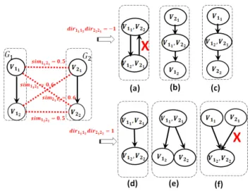
SS2 (Edge Direction) The purpose of this constraint is to prevent the generation of conflictual edges. On the left side of Fig.4, we have two input graphs G1 and G2, on the right side we have two sets of possible integration situations which depend on the product of edges’ directions. When the product’s edges’ direction is equal to 1, we notice that we have situations similar to those previously explained in the constraint SS1. When product’s edges’ direction is equal to -1, we notice case (a), in which the integrated graph is no longer simple. To generate simple integrated graphs, we propose the following constraint, which will be applied when edges’ direction is equal to -1: ∀i ∈ [1, N − 1], j ∈ [i + 1, N ] such as ∀k, k0 ∈ [1, ni] ∀l, l0∈ [1, nj]
xik,jl+ xik0,jl0+ (dirik,k0dirjl,l0) ≤ 0
Example 4. The SS2 constraints generated for the example of Fig.4 is :
x11,22+ x12,21+ (dir11,2dir22,1) ≤ 0 (5)
x11,21+ x12,22+ (dir11,2dir21,2) ≤ 0 (6)
◦ If x11,22 = 1 and x12,21 = 1 , knowing that
we have dir11,2 = −1 and dir22,1= −1 Then
constraint (5) is not satisfied (1 ≤ 0) . This case corresponds to situation (a) in Fig.4. 3) Resulting Model: The objective of our model is to maximize the sum of the similarities between matched vertices. Using the constraints mentioned above, our resulting model is as follows: max N −1 X i=1 N X j=i+1 ni X k=1 nj X l=1 simik,jlxik,jl s.t. nj X l=1 xik,jl≤ 1, ∀k ∈ [1, ni] (M S1) ∀i ∈ [1, N − 1], j ∈ [i + 1, N ] simik,jlxik,jl≥ thresh xik,jl (M S2) ∀i ∈ [1, N − 1], j ∈ [i + 1, N ] ∀k ∈ [1, ni], ∀l ∈ [1, nj] xik,jl≤ xipred(k),jpred(l) (SS1) ∀i ∈ [1, N − 1], j ∈ [i + 1, N ] ∀k ∈ [1, ni], ∀l ∈ [1, nj] xik,jl+ xik0,jl0− (dirik,k0dirjl,l0) ≤ 1 (SS2) ∀i ∈ [1, N − 1], j ∈ [i + 1, N ] ∀k, k0∈ [1, ni], ∀l, l0∈ [1, nj] xik,jl∈ {0, 1} ∀i ∈ [1, N − 1], j ∈ [i + 1, N ] ∀k ∈ [1, ni], ∀l ∈ [1, nj] Our model has:
Fig. 4. Example of Edge Direction Constraint Impact
• PN −1i=1 PNj=i+1ninj decision variables • PNi=1ni (N − i) constraints of type MS1. • The constraints MS2 arePNi=1ni− 1. • The constraints SS1 are ≤PN −1i=1 ni− 1.
• The constraints SS2 are ≤PN −1i=1 PNj=i+1|Ei||Ej|. The LP4HM program focuses on 1:1 matching cardinalities using 0-1 decision variables. We propose to relax the decision variables in the [0,1] interval. This relaxation enables resolving n:m matching cardinalities. Suppose that we have two vertices ”first name” and ”last name” both having the same similarity distance to ”name”. Therefore, we have two 0-1 decision variables with the same similarity factor, only one of these decision variables will be chosen. By relaxing variables in the [0,1] interval both variables will be assigned with a 0.5 value. We named LP4HM(relax) a relaxed version of LP4HM with decision variables in [0,1] resolving complex matching cardinalities (n:m).
In the related work section, we have shown that almost all approaches require tuning threshold to improve their matching quality. We think that searching a global optimal solution can help us to overcome this problem. Hence, we propose that our default LP4HM runs without the constraint MS2. These propositions will be studied experimentally in the next section.
IV. EVALUATION
In this section, we present three types of evaluations conducted on the LP4HM program. In the first evaluation, we assess the pairwise matching quality of our approach compared to COMA++ [15], BMatch [17] and Similarity Flooding [16]. In the second evaluation, we provide an estimation of the global optimal solution compared to a generalisation of local optimal solutions in the case of holistic matching. In the last evaluation, we test the performance of our approach according to running time resolution on several input SOD graphs. Experimentations have been carried out on a Dell PC (windows 8, Intel(R) Core i5, 2,30 Ghz processor, 8 Go RAM) and resolved by the Academic CPLEX solver.
A. Matching Quality
Given the absence of holistic tools adapted for hierarchical schemas, we have chosen to compare the matching quality of LP4HM with some pairwise approaches. The selected ap-proaches are COMA++, BMatch and Similarity Flooding (SF). All of them handle hierarchical schemas. The comparative study is conducted on the user-oriented benchmark6 proposed by [16]. The benchmark is composed of nine pairwise match-ing tasks. Tasks 1, 2, 3, 4, 5 and 6 are XML and XSD schemas and tasks 7, 8, 9 are relational database schemas. Seven users from the Stanford Database Group have proposed correspondences of cardinality 0:n for each of these tasks.
We have experimented on this benchmark: (i) our approach LP4HM without the threshold constraint; (ii) our relaxed approach LP4HM(Relax) without the threshold constraint; (iii) COMA++ by combining all the proposed strategies except the reuse and fragmentation ones; (iv) the default version of BMatch and (v) the SF7 algorithm implemented in the RONDO8 tool with a threshold equals to 1 as its authors rec-ommended it [16]. We highlight that even if the recrec-ommended threshold in SF seems evident in this benchmark, it is not generalizable and efficient for other tasks, for instance, the results of SF on the benchmark proposed by [28]. Moreover, we point out that we cannot compare local and global optimum in this benchmark, especially between SF and our approach. For doing that, the approaches should be subject to the same input sets and the same conditions, which is not the case here. Indeed, we use different seed element-level matchers so different input sets. Moreover, SF uses a threshold and LP4HM does not use a threshold so the conditions are different too.
The matching quality is evaluated by two classes of mea-sure. The first one is composed by precision, recall and f-measure, which are the classical measures of the Information Retrieval domain. Precision is defined as the ratio of correct correspondences to the total number of correspondences re-trieved by the system. The recall is defined as the ratio of the correct correspondences to the total number of correspon-dences proposed by the user. F-Measure is a harmonic mean of precision and recall. The second class is composed by accuracy [16] and HSR [28], which evaluate the post-match effort that a given user could save.
Some correlations exist between these measures. For in-stance, precision is correlated to accuracy. The authors of SF [16] affirm that accuracy decreases (negative results) if the precision is lower than 50%. Also, recall and precision are inversely correlated, so the f-measure is considered as the compromise between them.
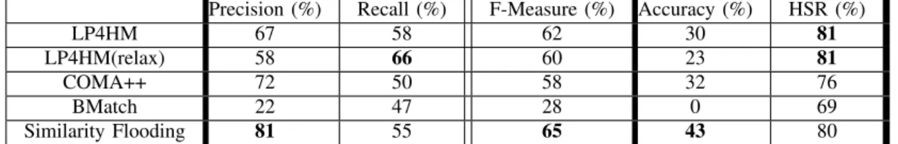
Table II summarizes the results of the different quality measures per average task and per average user for all ap-proaches. The authors of SF have chosen a high threshold so their results are focused on precision, which explains their good results on accuracy (the correlated measure to precision). However, we have intentionally make the choice to experiment our approach without threshold, so it is trivial
6http://infolab.stanford.edu/∼melnik/mm/sfa/
7We note that the recomputed accuracy results of SF are slightly different
from those published in [16]. We think that this is due to the use of the RONDO default functions.
TABLE II. THE QUALITY MEASURES VALUES PER AVERAGE TASK AND PER AVERAGE USER
Precision (%) Recall (%) F-Measure (%) Accuracy (%) HSR (%)
LP4HM 67 58 62 30 81
LP4HM(relax) 58 66 60 23 81
COMA++ 72 50 58 32 76
BMatch 22 47 28 0 69
Similarity Flooding 81 55 65 43 80
that our approach will not be the best on precision. Our approach will search a global optimal solution in all the space of solutions unconditioned with a threshold, so it is likely possible that some correspondences with low similarities will be selected in the global solution so for some users and for some tasks our approach will give not correct correspondences. Even if our approach without threshold has this bias, we can observe that our approach, especially the LP4HM(Relax), is better than SF in the recall measure, which is more significant than precision for users because it is computed based on their proposed correspondences. If we examine the compromise between precision and recall given by the f-measure, we can indeed observe that our approach reaches a very close results compared to SF even without threshold. This shows that our results are competitive to SF, even though, there are differences in the results of precision and recall.
For the post-match effort, like the authors of [28], we think that HSR is more significant than accuracy, first because it takes into account the number of elements of the schemas, second because it does not penalize the low results of precision like accuracy. Readers can simply observe that for the BMatch approach has 0% accuracy and 69% HSR. Our results on HSR are very close to SF too, which also shows that our approach and SF have competitive results. We point out that the HSR results of our approach and SF reveal more than 80% of post-match effort gained.
For our approach, we can observe that LP4HM(relax) version has better results on recall and lower results in precision compared to LP4HM version. Indeed, the set of found correspondences of LP4HM(relax) is larger than that of LP4HM. So for the same set of correct correspondences, the precision of LP4HM(Relax) will be lower than that of LP4HM. Moreover, if users give n:m correspondences then the set of correct correspondences of LP4HM(relax) will be larger than that of LP4HM. So the recall of LP4HM(Relax) will be greater than that of LP4HM.
In the following, we show more detailed results as depicted in Fig.5(a)-(j). We analyse results, first, along the different tasks for an average user, second, along the different users for an average task.
Fig.5(a) and Fig.5(c) depict precision and recall by task for an average user. We point out that tasks 1, 7, 8 and 9 have flat structures compared to the nested structures (depth ≥ 3) of the tasks 2, 3, 4, 5 and 6. We observe that nested tasks are more difficult than flat tasks. LP4HM and LP4HM(relax) perform medium precision results with few exceptions. For instance, precision in task 2 is high due to the use of linguistic measures. In turn, LP4HM(relax) performs good recall results for most tasks in particular for nested tasks. For tasks 7 and 8 we have lost some information, such as the datatypes, when
we fitted relational database schemas into our graphs. From this our results are lower than SF results. Task 9 consists of matching 5 tables in the left schema to one table in the right schema. For this task, our matcher, COMA++ and SF, found the correct correspondences to the right schema providing precise results. However, recall results are low due to several inconsistencies and differences between the correspondences proposed by users.
Precision and recall per users for an average task are depicted respectively in Fig.5(b) and Fig.5(d). We can see in Fig.5(b) that the precision of LP4HM is better than the precision of LP4HM(relax) for all users. In turn, the recall of LP4HM(relax) is better than the recall of LP4HM for all users. The recall of our approach is better than that of COMA++, BMatch and SF for all users. To summarize, LP4HM is more precise than LP4HM(relax) because the former focuses on 1:1 matching cardinalities and the latter focuses on n:m matching. Contrarily, for the same reason LP4HM(relax) better meets the users that have performed 0:n correspondences.
We notice in Fig.5(g) that some accuracy results of our approach are very low. This is due to precision results that are lower than 50% [16]. In Fig.5(h), though, the accuracy results per user are close to COMA++ and SF results. Finally, for the HSR results, both LP4HM and LP4HM(relax) perform the best results in Fig.5(i) and in Fig.5(j).
We conclude that both LP4HM and LP4HM(relax) show experimentally competitive results for different users and dif-ferent matching tasks compared to SF, COMA++ and BMatch approaches. LP4HM is more precise than LP4HM(relax), but the recall of LP4HM(relax) is better than the recall of LP4HM. Both approaches perform good matching of nested tasks and good results on HSR and accuracy for the post-match effort.
Searching global optimal solution is an efficient strategy since this allows our approach to face other approaches without having to use a threshold. Users seem unanimously apprecia-tive of the effecapprecia-tiveness of our approach in particular for recall and HSR. The encouraging results on the nested tasks respond exactly to a major problem we try to solve, which is integrating hierarchical Open Data structures. Finally, we think that having good recall is an interesting indicator for holistic matching. Indeed, if precision is better than recall so users have to find the missing correspondences for N schemas simultaneously, which is a human difficult task. So when system returns good recall and moderate precision, users have just to eliminate the not relevant mappings proposed by the matcher.
B. Global Optimum and Local Optimum In holistic Matching In this section, we compare the global optimal solution of our approach and the sum of local optimal solutions of the SF [16] approach, in a simple case study of holistic matching.
(a) Precision per task for average user (b) Precision per user for average task
(c) Recall per task for average user (d) Recall per user for average task
(e) F-Measure per task for average user (f) F-Measure per user for average task
(g) Accuracy per task for average user (h) Accuracy per user for average task
(i) HSR per task for average user (j) HSR per user for average task Fig. 5. Quality Measures Comparison between LP4HM, LP4HM(Relax), COMA++, BMatch, SF
The case study consists of matching some SOD tables dealing with drugs seizure in United Kingdom. The graphs G1, G2 and G3, in Fig.6, show an excerpt of these tables. The data of G1are extracted from the Scotland provider9. The data of graphs G2 and G3 are extracted from the UK provider10. We have computed similarities between the different nodes of the graphs (the non-specified similarities are considered as null values) and injected them to both approaches. Both approaches are used with a 0 threshold. The SF apply its propagation algorithm to compute structural similarities on the basis of injected similarities. Then, it applies its filter and extract correspondences. Our approach resolves an ILP maximizing the same input similarities under linear constraints on the structures of the graphs. The correspondences are the solutions of the ILP.
Fig. 6. A simple case study of holistic matching
The solution of the SF approach is the union of the solutions of three pairwise matching problems as follows:
• M atch(G1, G2) → {(v11, v21) = 0.35}; • M atch(G1, G3) → {(v11, v31) = 0.79};
• M atch(G2, G3) → {(v21, v31) = 0.62, (v22, v32) = 1, (v23, v33) = 1}.
The solution our approach LP4HM corresponds to one run taking as input G1, G2 and G3 and returning the following correspondences:
• M atch(G1, G2, G3) → {(v12, v21) = 0.7 , (v12, v31) = 0.52, (v21, v31) = 0.62, (v22, v32) =
1, (v23, v33) = 1}.
We can observe that the the sum of similarities (3.76) of the SF solution is lower than the sum of similarities (3.84) of LP4HM solution. These results support the idea that global optimal solutions represent a promising strategy for holistic schema matching problems.
9
http://www.scotland.gov.uk/Topics/Statistics/Browse/Crime-Justice/TrendData
10http://data.gov.uk/dataset/seizures-drugs-england-wales
C. Matching Performance
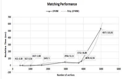
We evaluate the matching performance by studying the resolution time as a function of the size (number of vertices) of several input SOD graphs. Considering that our approach performs matching only on structural data, the size of each in-putted graph is not very large. Indeed, in our running example for each source, structural data represents merely 12% of the total amount of information (structural and numerical data). So, the total size of inputted graphs in our experimentation is significant for our automatic integration study on SOD.
Fig. 7. Resolution time as a function of number of vertices
We have experimented LP4HM for a holistic integration of the graphs of our motivating example. We remind readers that these graphs were generated automatically from the first step of our ETL processes. The LP4HM model was solved using the Cplex solver. Fig.7 depicts the resolution time as a function of the number of vertices of several input graphs. The continuous curve connects the measured values and the discontinuous curve is a trend-line of the first one. We can observe, experimentally, that the resolution time has a poly-nomial trend-line O(n4) according to the number of vertices. These results join the polynomial dissertation of [24] about the weighted graph matching problem, even though we have used a different technique. We can notice that for 415 vertices (9 input schemas), our model found a solution in 0,38 sec. Moreover, when the size of graphs grows up to 4977 vertices (46 input schemas), the linear program found a solution in 533,95 sec 9,23 mn, which is a reasonable automatic resolution time with respect to time users need to do such a tedious task manually. To conclude, our approach LP4HM is able to match N SOD graphs in an affordable time for an important size of structural graphs.
V. CONCLUSION
In this paper, we presented an integer linear program, named LP4HM, performing holistic Statistical Open Data (SOD) graph matching. This program is part of our graph-based ETL approach proposed to warehouse SOD. LP4HM is and extension of the weighted graph matching problem with different constraints on graph structures and matching setup, especially 1:1 matching. We have performed a user-oriented benchmark on LP4HM and some other approaches
in the literature. The comparative experimentations show the effectiveness of LP4HM without threshold tuning and the LP4HM(relax) that is a relaxation of our model able to resolve complex matching cardinalities. Moreover, we have demon-strated the importance of globally optimal solutions compared to locally optimal solutions in a holistic case. LP4HM shows a reasonable resolution time for several input graphs.
For future work, we will extend our linear program with some constraints related to properties of graph labels. We aim to handle the specificities of ontologies in our model. Further-more, some algorithms in the combinatorial optimisation field will be tested in order to make a comparative study on the performance of our model on very large problems.
REFERENCES
[1] A. Berro, I. Megdiche, and O. Teste, “A content-driven ETL processes for open data,” in New Trends in Database and Information Systems II, Selected papers of the 18th East European Conference on Advances in Databases and Information Systems, ADBIS’14. Springer International Publishing, 2014, vol. 312, pp. 29–40.
[2] E. Rahm and P. A. Bernstein, “A survey of approaches to automatic schema matching,” VLDB JOURNAL, vol. 10, 2001.
[3] R. Angles and C. Gutierrez, “Survey of graph database models,” ACM Comput. Surv., vol. 40, no. 1, p. 139, 2008.
[4] A. Berro, I. Megdiche, and O. Teste, “Graph-based etl processes for warehousing statistical open data,” in ICEIS 2015, 2015, pp. 271–278. [5] F. Ravat, O. Teste, R. Tournier, and G. Zurfluh, “Graphical querying of
multidimensional databases,” in ADBIS 2007, 2007, pp. 298–313. [6] E. Malinowski and E. Zim´anyi, “Hierarchies in a multidimensional
model: From conceptual modeling to logical representation,” Data Knowl. Eng., vol. 59, no. 2, pp. 348–377, 2006.
[7] E. Rahm, “Towards large-scale schema and ontology matching,” in Schema Matching and Mapping, ser. Data-Centric Systems and Ap-plications, Z. Bellahsene, A. Bonifati, and E. Rahm, Eds. Springer Berlin Heidelberg, 2011, pp. 3–27.
[8] P. Shvaiko and J. Euzenat, “A survey of schema-based matching approaches,” in Journal on Data Semantics IV. Springer Berlin Heidelberg, 2005, pp. 146–171.
[9] B. He and K. C. Chang, “Automatic complex schema matching across web query interfaces: A correlation mining approach,” ACM Trans. Database Syst., vol. 31, no. 1, pp. 346–395, 2006.
[10] W. Su, J. Wang, and F. H. Lochovsky, “Holistic schema matching for web query interfaces,” in Advances in Database Technology -EDBT 2006, 10th International Conference on Extending Database Technology, Munich, Germany, March 26-31, 2006, Proceedings, 2006, pp. 77–94.
[11] K. Saleem, Z. Bellahsene, and E. Hunt, “Performance oriented schema matching.” in DEXA, vol. 4653, 2007, pp. 844–853.
[12] A. Benharkat, R. Rifaieh, S. Sellami, M. Boukhebouze, and Y. Amghar, “PLASMA: A platform for schema matching and management,” IBIS, vol. 5, pp. 9–20, 2007.
[13] A. Termier, M.-C. Rousset, and M. Sebag, “Dryade: a new approach for discovering closed frequent trees in heterogeneous tree databases,” in Data Mining, 2004. ICDM ’04. Fourth IEEE International Conference on, Nov 2004, pp. 543–546.
[14] U. Chukmol, R. Rifaieh, and N. Benharkat, “Exsmal: Edi/xml semi-automatic schema matching algorithm,” in E-Commerce Technology, 2005. CEC 2005. Seventh IEEE International Conference on, July 2005, pp. 422–425.
[15] D. Aumueller, H.-H. Do, S. Massmann, and E. Rahm, “Schema and ontology matching with coma++,” in SIGMOD ’05, 2005, pp. 906–908. [16] S. Melnik, H. Garcia-Molina, and E. Rahm, “Similarity flooding: A versatile graph matching algorithm and its application to schema matching,” in Proceedings of the 18th International Conference on Data Engineering, ser. ICDE ’02. IEEE Computer Society, 2002, pp. 117–.
[17] F. Duchateau, Z. Bellahsene, and M. Roche, “Bmatch: a semantically context-based tool enhanced by an indexing structure to accelerate schema matching,” in 23`emes Journ´ees Bases de Donn´ees Avanc´ees, BDA 2007, Marseille, 23-26 Octobre 2007, Actes (Informal Proceed-ings), 2007.
[18] J. Huber, T. Sztyler, J. Nner, and C. Meilicke, “Codi: Combinatorial optimization for data integration: results for oaei 2011.” in OM, ser. CEUR Workshop Proceedings, vol. 814. CEUR-WS.org, 2011. [19] J. Euzenat and P. Valtchev, “Similarity-based ontology alignment in
owl-lite,” in Proc. 16th european conference on artificial intelligence (ECAI), Valencia (ES). IOS press, 2004, pp. 333–337.
[20] J. Euzenat and P. Shvaiko, Ontology matching, 2nd ed. Heidelberg (DE): Springer-Verlag, 2013.
[21] M. Niepert, C. Meilicke, and H. Stuckenschmidt, “A Probabilistic-Logical Framework for Ontology Matching,” in Proceedings of the 24th AAAI Conference on Artificial Intelligence. AAAI Press, 2010, pp. 1413–1418.
[22] A. Schrijver, Combinatorial Optimization - Polyhedra and Efficiency. Springer, 2003.
[23] H. A. Almohamad and S. Duffuaa, “A linear programming approach for the weighted graph matching problem,” IEEE Trans. Pattern Anal. Mach. Intell, pp. 522–525, 1993.
[24] J. Edmonds, “Maximum matching and a polyhedron with 0, 1-vertices,” Journal of Research of the National Bureau of Standards B, vol. 69, pp. 125–130, 1965.
[25] Z. Wu and M. Palmer., “Verb semantics and lexical selection.” in In 32nd. Annual Meeting of the Association for Computational Linguistics, 1994, pp. 133–138.
[26] D. Lin, “An information-theoretic definition of similarity,” in In Pro-ceedings of the 15th International Conference on Machine Learning. Morgan Kaufmann, 1998, pp. 296–304.
[27] F. Plastria, “Formulating logical implications in combinatorial optimi-sation,” European Journal of Operational Research, vol. 140, no. 2, pp. 338 – 353, 2002.
[28] F. Duchateau and Z. Bellahsene, “Designing a benchmark for the assessment of schema matching tools,” Open Journal of Databases (OJDB), vol. 1, no. 1, pp. 3–25, 2014.