Predicting Aircraft Descent Length with Machine Learning

O

pen

A

rchive

T

OULOUSE

A

rchive

O

uverte (

OATAO

)

OATAO is an open access repository that collects the work of Toulouse researchers and

makes it freely available over the web where possible.

This is an author-deposited version published in :

http://oatao.univ-toulouse.fr/

Eprints ID : 17232

The contribution was presented at ICRAT 2016:

http://www.icrat.org/icrat/

To cite this version :

Alligier, Richard and Gianazza, David and Durand, Nicolas

Predicting Aircraft Descent Length with Machine Learning. (2016) In: 7th

International Conference on Research in Air Transportation (ICRAT 2016), 20

June 2016 - 24 June 2016 (Philadelphia, United States).

Any correspondence concerning this service should be sent to the repository

administrator:

staff-oatao@listes-diff.inp-toulouse.fr

Predicting Aircraft Descent Length with Machine

Learning

R. Alligier, D. Gianazza, N. Durand

ENAC, MAIAA, F-31055 Toulouse, France Univ. de Toulouse, IRIT/APO, F-31400 Toulouse, France

Abstract—Predicting aircraft trajectories is a key element in the detection and resolution of air traffic conflicts. In this paper, we focus on the ground-based prediction of final descents toward the destination airport. Several Machine Learning methods – ridge regression, neural networks, and gradient-boosting ma-chine – are applied to the prediction of descents toward Toulouse airport (France), and compared with a baseline method relying on the Eurocontrol Base of Aircraft Data (BADA).

Using a dataset of 15,802 Mode-S radar trajectories of 11 different aircraft types, we build models which predict the total descent length from the cruise altitude to a given final altitude. Our results show that the Machine Learning methods improve the root mean square error on the predicted descent length of at least 20 % for the ridge regression, and up to 24 % for the gradient-boosting machine, when compared with the baseline BADA method.

Keywords: aircraft trajectory prediction, descent, BADA, Machine Learning

INTRODUCTION

An accurate trajectory prediction (TP) is a prerequisite to any operational implementation of conflict detection and reso-lution (CDR) algorithms. Most current trajectory predictors use a point-mass model of the aircraft that requires input parameters such as the aircraft mass, thrust and speed intent. Unfortunately, these data are often uncertain or even unknown to ground-based predictors which use default values instead, leading to poor predictions. As shown in [1], the performance of CDR algorithms is highly impacted by uncertainties in the trajectory prediction.

One could think that downloading the on-board FMS pre-diction would solve this issue. This is not true however, as ground-based applications may need to search among a large number of alternative trajectories to find an optimal solution to a given problem. For example, in [2] an iterative quasi-Newton method is used to find trajectories for departing aircraft, minimizing the noise nuisance. Another example is [3] where Monte Carlo simulations are used to estimate the risk of conflict between trajectories in a stochastic environment. Some of the automated tools currently being developed for ATM/ATC can detect and solve conflicts between trajectories (see [4] for a review). These algorithms may use Mixed Integer Programming ([5]), Genetic Algorithms ([6], [7]), Ant Colonies ([8]), or Differential Evolution or Particle Swarm Optimization ([9]) to find optimal solutions to air traffic conflicts. The on-board computers and the datalink capabilities are currently not fit to the purpose of transmitting a large

number of alternative trajectories, as would be required by such applications.

Another obvious solution would be to downlink the point-mass model parameters to ground-based systems. However, some of these parameters (mass, speed intent) are considered as competitive by some airline operators which are reluctant to transmit them. One can hope that these on-board parameters will be made available in the future. In the meantime, air nav-igation service providers are left with work-around solutions to improve their ground-based trajectory predictors.

In previous works [10], [11], we used a Machine Learning approach to improve the altitude prediction of climbing air-craft. The proposed approach consisted in learning models that could estimate the missing parameters, or directly predict the future altitude. We now propose to apply Machine Learning techniques to the prediction of descents towards the destination airport.

In the current paper, we address the descent prediction problem with neural networks (NNet), gradient-boosted ma-chines (GBM), and ridge regression (Ridge) methods and compare the results with a baseline method relying on the Eurocontrol BADA model. These methods are compared using a 10-fold cross-validation on a dataset of 15,802 Mode-S radar trajectories comprising 11 aircraft types.

The sequel of this paper is organized as follows: Section I describes the background and problem statement. Section II presents some useful Machine Learning notions that help understanding the methodology applied in our work. The methods applied to our descent length prediction problem are described in section III. Section IV details the data used in this study, and the results are shown and discussed in section V, before the conclusion.

I. BACKGROUND AND PROBLEM STATEMENT

Predicting the aircraft final descent toward the airport is a crucial problem that has been already studied, for example in the context of the evaluation of a descent advisory tool [12], [13], or an operational trajectory predictor [14]. In [14], the predictions of a Eurocat Trajectory Predictor are com-pared with the actual trajectories of 51 continuous descents to Stockhom-Arlanda airport, considering one aircraft type (B737) operated by a single company. The influence of various additional data on the prediction accuracy is studied. The study concluded that FMS 4D-trajectory was the main source of improvement, followed by the aircraft mass. Surprisingly, the

questioning how the TP logic takes these data into account. In [15], Stell applies a linear regression method to a dataset of about 70 idle-thrust descent trajectories per aircraft type considered in the study (A319/320, B757). All the flights were descending toward Denver International Airport and belonged to a same airline. For each flight, the descent speed intent and aircraft mass are known and used in the study. These works conclude that a linear combination of the explanatory variables (cruise and meter fix altitudes, descent CAS, wind, and possibly weight, for the Airbus) could successfully predict the top-of-descent. However, the experimental setup required to collect the data from many different sources over a short period (3 weeks). A relatively small amount of data was collected, that might not cover the actual range of all parameter values.

In [16], the same operational data is used, and also some laboratory data obtained from FMS test benches for two aircraft types (B737-700 and B777-200). The author makes polynomial and linear approximations of the distance from TOD to meter fix computed by the EDA (Efficient Descent Advisor) tool, for these two aircraft types. The conclusion is that a polynomial or even a linear model can efficiently approximate this along-track distance using the cruise altitude, descent CAS, aircraft weight, wind, and the altitude and velocity at the meter fix as explanatory variables.

In [17], Stell et al. use a larger dataset with 1088 flights of a single aircraft type (B737-800), with two different motoriza-tions. The aircraft masses were not collected. The Intermediate Projected Intent (IPI) is extracted from ADS-C data and used to determine the actual top-of-descent, as well as the initial cruise and final altitudes, and the descent CAS. Several canditate linear or polynomial models predicting the TOD from various subsets of variables are fitted on the data. The subsets of variables comprise the cruise and final altitudes, the cruise mach number, descent CAS, and forecast wind. After a thorough analysis, the paper concludes that simple linear models using the cruise and final altitudes and CAS intent could be the basis of further work in order to use them in decision support tools.

In the current paper, we investigate how Machine Learning techniques could improve the prediction of the final descent toward the destination airport. A dataset of trajectory examples is used to tune different models (linear models, neural net-works, gradient boosting machines) predicting the total length of descent between the cruise altitude and a final altitude which is either FL150 or the altitude at which the descent is interrupted by a intermediate leveled flight segment. Our dataset comprises 15,802 trajectories of 11 different aircraft types (A319, A320, A321, A3ST, B733, B738, CRJ1, CRJ7, CRJ9, CRJX and E190). The trajectories were recorded from the Toulouse Mode-S radar data, in the south of France. The aircraft masses are not available as we use only Mode-S data. The wind data is extracted from the ground speed and true airspeed downlinked from the aircraft. The actual descent speed could have been extracted from each Mode-S example trajectory by adjusting it on the observed data. This was not done in this study however. Using the speed intent in our

The purpose of the current preliminary study is to evaluate the performances of several Machine Learning techniques on the total descent length prediction problem, and to compare them with a baseline method relying on the 3.13 release of the Eurocontrol Base of Aircraft Data (BADA) [18].

II. MACHINELEARNING

This section describes some useful Machine Learning no-tions and techniques. For a more detailed and comprehensive description of these techniques, one can refer to [19], [20].

We want to predict a variable y, here the descent length, from a vector of explanatory variables x, which in our case is the data extracted from the past trajectory points and the weather data. This is typically a regression problem. Naively said, we want to learn a function h such that y = h(x) for all(x, y) drawn from the distribution (X, Y ). Actually, such a function does not exist, in general. For instance, if two ordered pairs (x, y1) and (x, y2) can be drawn with y1 6= y2, h(x)

cannot be equal to y1and y2at the same time. In this situation,

it is hard to decide which value to give to h(x).

A way to solve this issue is to use a real-valued loss function L. This function is defined by the user of function h. The value L(h(x), y) models a cost for the specific use of h when (x, y) is drawn. With this definition, the user wants a function h minimizing the expected loss R(h) defined by equation (1). The value R(h) is also called the expected risk.

R(h) = E(X,Y )[L (h(X), Y )] (1)

However, the main issue when choosing a function h minimiz-ing R(h) is that we do not know the joint distribution (X, Y ). We only have a set of examples of this distribution.

A. Learning from examples

Let us consider a set of n examples S = (xi, yi)16i6n

coming from independent draws of the same joint distribution (X, Y ). We can define the empirical risk Rempirical by the

equation below: Rempirical(h, S) = 1 |S| X (x,y)∈S L(h(x), y) . (2) Assuming that the values(L(h(x), y))(x,y)∈S are independent

draws from the same law with a finite mean and variance, we can apply the law of large numbers giving us that Rempirical(h, S) converges to R(h) as |S| approaches +∞.

Thereby, the empirical risk is closely related to the expected risk. So, if we have to select h among a set of functions H minimizing R(h), using a set of examples S, we select h minimizing Rempirical(h, S). This principle is called the

principle of empirical risk minimization.

Unfortunately, choosing h minimizing Rempirical(h, S) will

not always give us h minimizing R(h). Actually, it depends on the “size”1_{of H and the number of examples|S| ([21], [22]).}

1_{The “size” of H refers here to the complexity of the candidate models}

contained in H, and hence to their capability to adjust to complex data. As an example, if H is a set of polynomial functions, we can define the “size” of H as the highest degree of the functions contained in H. In classification problems, the “size” of H can be formalized as the Vapnik-Chervonenkis dimension.

The smaller H and the larger|S| are, the more the principle of

empirical risk minimizationis relevant. When these conditions

are not satisfied, the selected h will probably have a high R(h) despite a low Rempirical(h, S). In this case, the function h is

overfittingthe examples S.

These general considerations have practical consequences on the use of Machine Learning. Let us denote hS the function

in H minimizing Rempirical(., S). The expected risk using hS

is given by R(hS). We use the principle of empirical risk

minimization. As stated above, some conditions are required for this principle to be relevant. Concerning the size of the set of examples S: the larger, the better. Concerning the size of H, there is a trade off: the larger H is, the smaller min

h∈H R(h)

is. However, the larger H is, the larger the gap between R(hS)

and min

h∈H R(h) becomes. This is often referred to as the

bias-variance trade off. B. Accuracy Estimation

In this subsection, we want to estimate the accuracy ob-tained using a Machine Learning algorithm A. Let us denote A[S] the prediction model found by algorithm A when mini-mizing Rempirical(., S)2, considering a set of examples S.

The empirical risk Rempirical(A[S], S) is not a suitable

estimation of R(A[S]): the law of large numbers does not apply here because the predictor A[S] is neither fixed nor independent from the set of examples S.

One way to handle this is to split the set of examples S into two independent subsets: a training set ST and another

set SV that is used to estimate the expected risk ofA[ST], the

model learned on the training set ST. For this purpose, one

can compute the holdout validation error Errvalas defined by

the equation below:

Errval(A, ST, SV) = Rempirical(A[ST], SV). (3)

Cross-validation is another popular method that can be used to estimate the expected risk obtained with a given learning algorithm. In a k-fold cross-validation method, the set of examples S is partitioned into k folds(Si)_16i6k. Let us denote

S−i= S\Si. In this method, k trainings are performed in order

to obtain the k predictors A[S−i]. The mean of the holdout

validation errors is computed, giving us the cross-validation estimation below: CVk(A, S) = k X i=1 |Si|

|S|Errval(A, S−i, Si). (4) This method is more computationally expensive than the holdout method but the cross-validation is more accurate than the holdout method ([23]). In our experiments, the folds were stratified. This technique is said to give more accurate estimates ([24]).

The accuracy estimation has basically two purposes: first, model selection in which we select the “best” model using

2_{Actually, depending on the nature of the minimization problem and}

chosen algorithm, this predictorA[S] might not be the global optimum for Rempirical(., S), especially if the underlying optimization problem is handled

by local optimization methods.

accuracy measurements and second, model assessment in which we estimate the accuracy of the selected model. For model selection, the set SV in Errval(A, ST, SV) is called

validation setwhereas in model assessment this set is called

testing set.

C. Hyperparameter Tuning

Some learning algorithms have hyperparameters. These hy-perparameters λ are the parameters of the learning algorithm Aλ. These parameters cannot be adjusted using the empirical

risk because most of the hyperparameters are directly or indirectly related to the size of H. Thus, if the empirical risk was used, the selected hyperparameters would always be the ones associated to the largest H.

These hyperparameters allow us to control the size of H in order to deal with the bias-variance trade off. These hyperpa-rameters can be tuned using a cross-validation method on the

training setfor accuracy estimation. This accuracy estimation

is used for model selection. In order to select a value of λ minimizing this accuracy estimation, we used a grid search which consists in an exhaustive search in a grid of hyper-parameter values. In the Algorithm 1, T uneGrid(Aλ, grid)

is a learning algorithm without any hyperparameters. In this algorithm, a 10-fold cross-validation is used on the training setto select the hyperparameters λ for the algorithm Aλ.

function TUNEGRID(Aλ,grid)[T ]

λ∗_{← argmin} λ∈grid

CV10(Aλ, T)

returnAλ∗[T ] end function

Algorithm 1: Hyperparameters tuning for an algorithmAλand

a set of examples T (training set).

III. MACHINELEARNINGMETHODS

In this section, we briefly describe the Machine Learning techniques applied to our descent length prediction problem.

A. Ridge Regression (Ridge)

Linear regression ([25], [26]) is a widely used method. With this method, the set of functions H contains all the linear functions. Thus, if we consider that x is a tuple of p values (x1, ..., xi, ..., xp), the prediction h(x; θ) is expressed

as follows: h(x; θ) = p X i=1 θixi+ θ0 (5)

where θ is a tuple of p+ 1 values. From the training set, the parameters θ are estimated by minimizing the sum of squared error. When the loss function is the square function, the estimated parameter is also the one minimizing the empirical risk. However, when some variables of x are nearly collinear, the estimation of θ using the least square method might give a high expected risk even if the empirical risk was low. To

parameters by minimizing the following expression: X (x,y)∈T (h(x; θ) − y)2+ λ p X i=1 θi2 (6)

where λ is an hyperparameter that must be selected by cross-validation. This parameter limits the range of the parameters θ. The larger λ is, the closer to zero the θi are. The

hyperpa-rameter grid used for this algorithm is presented in Table I.

method hyperparameter grid

Ridge_λ λ= 10J−7;1K_{∪ 0.5 × 10}J−7;0K

Table I: Grid of hyperparameters used in our experiments for Ridge.

B. Regression using Neural Networks (NNet)

Artificial neural networks are algorithms inspired from the biological neurons and synaptic links. An artificial neural network is a graph, with vertices (neurons, or units) and edges (connections) between vertices. There are many types of such networks, associated to a wide range of applications. Beyond the similarities with the biological model, an artificial neural network may be viewed as a statistical processor, making probabilistic assumptions about data ([28]). The reader can refer to [29] and [30] for an extensive presentation of neural networks for pattern recognition. In our experiments, we used a specific class of neural networks, referred to as feed-forward networks, or multi-layer perceptrons (MLP). In such networks, the units (neurons) are arranged in layers, so that all units in successive layers are fully connected. Multi-layers perceptrons have one input layer, one or several hidden layers, and an output layer. In our case, we have only one target value to predict, so the output layer has only one unit.

For a network with one hidden layer of n units and one unit on the output layer, the output h(x; θ) is expressed as a function of the input vector x = (x1, ..., xi, ..., xp)T as

follows: h(x; θ) = Ψ( n X j=1 θjΦ( p X i=1 θijxi+ θ0j) + θ0) (7)

where the θij and θj are weights assigned to the connections

between the input layer and the hidden layer, and between the hidden layer and the output layer, respectively, and where θ0j and θ0are biases (or threshold values in the activation of

a unit). Φ is an activation function, applied to the weighted output of the preceding layer (in that case, the input layer), and Ψ is a function applied, by each output unit, to the weighted sum of the activations of the hidden layer. This expression can be generalized to networks with several hidden layers.

The output error – i.e. the difference between the desired output (target values) and the output h(x; θ) computed by the network – will depend on the parameters θ (weights and biases), that must be tuned using a training set T . In order to minimize the expected risk and avoid overfitting, the weights and biases are tuned to minimize a regularized empirical risk

X (x,y)∈T (h(x; θ) − y)2+ λ n X j=1 p X i=1 θij2 (8)

where λ is a hyperparameter that must be selected by cross-validation. The larger λ is, the smoother h(.; θ) is. The method used to minimize this regularized empirical risk is a BFGS quasi-Newton method.

In our study, the activation function is the logistic sigmoïd, and the output function is the identity. The hyperparameter grid used for this algorithm is presented in Table II.

method hyperparameter grid NNet(n,λ)

n= {2, 3, 4, 5, 6, 7, 8, 9, 10}

λ= {0.0001, 0.0001, 0.001, 0.01, 0.1, 0.5, 1, 2, 5}

Table II: Grid of hyperparameters used in our experiments for NNet.

C. Gradient Boosting Machine (GBM)

The stochastic gradient boosting machine algorithm was introduced in [31]. It applies functional gradient descent ([32] using regression trees [33].

The functional gradient descent is a boosting technique. The model h is iteratively improved. At each iteration m we consider the opposite of the gradient of the loss gm,i =

−∂L(ˆy,yi)

∂yˆ (hm(xi) , yi). Using a regression tree algorithm

[33], a tree Tmpredicting gmis built from the set of examples

is(xi, gm,i)16i6n. Tm is a binary tree representing a binary

recursive partition of the input space. At each node, the input space is split into two regions according to a condition xj6s.

The J leaves describe a partition (Rj)_16j6J of the input

space. Each region Rjis associated to a constant γjand when

x falls into Rj, then γjis returned as the prediction result. The

updated model hm+1 predicting y is expressed as follows:

hm+1(x) = hm(x) + νTm(x) (9)

where ν is a learning rate that has to be tuned in order to avoid overfitting.

Regression trees have some advantages. The regression tree algorithm is insensitive to monotonic transformations of the inputs. Using xj, log(xj) or exp (xj) leads to the same model.

As a consequence, this algorithm is robust to outliers. It can easily handle categorical variables and missing values. However it is known to have a poor performance in prediction. The latter drawback is very limited when used in combina-tion with funccombina-tional gradient descent as it is done in the gradi-ent boosting machine algorithm. In our experimgradi-ents we used the gbm package ([34]) in the R software. This algorithm op-timizes the risk given by a quadratic loss L(ˆy, y) = (ˆy− y)2. Let us note GBM(M,J,ν,n) this algorithm, where M is the

number of boosting iterations, J is the number of leaves of the tree and ν is the shrinkage parameter. The obtained model is a sum of regression trees. J allows us to control the interaction between variables, as we have J− 1 variables at most in each regression tree. n is the minimum number of examples in each region Rj. The hyperparameter grid used for this algorithm is

method hyperparameter grid GBM(m,J,ν,n) M= {2000} J= {2, 3, 4, 6, 9, 11, 14, 16, 18} ν= {0.001, 0.0025, 0.005, 0.01} n= {3, 5, 10, 15}

Table III: Grid of hyperparameters used in our experiments for GBM.

IV. DATA USED IN THISSTUDY

A. Data Pre-processing

Mode-S data from the french air navigation service provider are used in this study. This Mode-S radar is located in the Toulouse area. This raw data is made of one position report every 4 to 5 seconds, over 242 days (from February 2011 to December 2012).

The trajectory data is made of the fields sent by the aircraft: aircraft position (latitude and longitude), altitude Hp (in feet

above isobar 1,013.25 hPa), rate of climb or descent, Mach number, bank angle, ground speed, true track angle, true airspeed and heading. The wind is computed from these last four variables, and the temperature is computed from the Mach number and the true airspeed. The raw Mode-S altitude has a precision of 25 feet. Raw data are smoothed using splines.

Along with these quantities derived from the Mode-S radar data, we have access to some quantities in the flight plan like the Requested Flight Level for instance.

B. Extracting the First Descent Segment

Only the flights arriving to Toulouse Blagnac (LFBO) are kept. The time tTOD at which the descent begins has to be

extracted from the radar track. To do so, the time with the highest altitude is determined. Starting from this time we search for the first time window of 1 min with a ROCD inferior to−200 ft/min. To obtain the time at which the descent begins, we add 10 s at the start of this time window. The descent segments with a Top Of Descent altitude H_pTOD inferior to 15,500 ft were discarded. The time tEODat which the descent

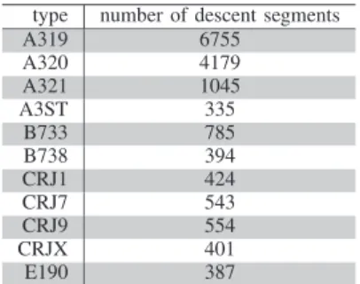
ends is the first time with a ROCD superior to −100 ft/min minus 30 s. If the ROCD is always inferior to this threshold till 15,000 ft, then we consider that the descent ends at 15,000 ft. Figure 1 illustrates the results of this algorithm for one day of traffic for the aircraft type A319. This process was applied to 11 different aircraft types. As summarized by table IV, we have obtained several hundred descent segments for each aircraft type. The variable to be predicted is the distance flown from tTOD to tEOD. This distance Sdesc is computed by

numerically integrating the smoothed ground speed between tTODand tEOD.

This process was applied to the trajectories of 11 different aircraft types. These aircraft types are the most highly repre-sented in our data set. Table IV summarizes the number of descent segments obtained.

C. The Explanatory Variables

We want to learn the distance flown during the first descent segment. The explanatory variables used to predict this target

type number of descent segments A319 6755 A320 4179 A321 1045 A3ST 335 B733 785 B738 394 CRJ1 424 CRJ7 543 CRJ9 554 CRJX 401 E190 387

Table IV: Size of the different sets of the descent segments.

0 10000 20000 30000 40000 0 1000

t − tTOD

[s]

H

[ft]

Figure 1: This figure illustrates one day of traffic for the aircraft type A319. The descent segments extracted are in blue.

variable are grouped in a tuple x. This tuple contains all the known variables when the aircraft is in cruise phase. We assume that the altitudes at the begining and the end of the descent are known. The wind and temperature at these altitudes can be easily computed from a weather forecast grid, prior to the descent phase. In our study, we do not have the a weather forecast. For want of anything better, these weather data are computed using the Mode-S radar data of the descent segment. Consequently, the distance errors presented in section V are probably smaller than what would be obtained with a forecast wind. However, our objective in this paper is only to compare the different methods and using the Mode-S wind should not significantly influence the results.

Knowing the departure and arrival airports, the distance and the track angle between these two airports are computed. In the hope of taking into account the impact of the wind on the distance flown, the wind at H_pTODis projected on the line segment between the two airports.

The variable dBADAis the distance predicted by BADA with

no wind and an ISA atmosphere. The variable dBADAw is the distance with the wind and the temperature computed from

that the lateral intent is known. Thus, in our study, we use the track angle and the bank angle computed from the Mode-S data. These two predicted distances are in the tuple x. The two predictions are added because we can consider that the difference between these two distances gives a good insight of the impact of the weather on the distance.

The QFU of the runway used by the aircraft is also in the tuple x. For each trajectory, this QFU is extracted from the radar data by taking the track angle at the point with the lowest altitude. If this heading is between 120 and 160, then the QFU is 140; if it is between 300 and 340 then the QFU is 320 otherwise the trajectory is discarded from our set of examples. Table V summarizes the explanatory variables used in this study.

quantities description

H_pTOD geopotential pressure altitude at tTOD

∆TTOD temperature differential at HpTOD

WTOD wind speed at HpTOD

W dirTOD wind direction at HpTOD

MachTOD Mach number at HpTOD

H_pEOD geopotential pressure altitude at tEOD

∆TEOD temperature differential at HpEOD

WEOD wind speed at HpEOD

W dirEOD wind direction at HpEOD

distance distance between airports

angle course between airports

windeffect wind along the track between

air-ports

RFL Requested Flight Level

Speed requested speed

QF U QFU of the runway used

dBADA distance predicted by BADA with no

wind and ISA atmosphere dBADAw distance predicted by BADA with the

actual weather

hour hour at which the aircraft lands month month at which the aircraft lands

Table V: Explanatory variables available in our study. V. RESULTS ANDDISCUSSION

All the statistics presented in this section are computed using a stratified 10-fold cross-validation embedding the hy-perparameter selection. Our set of examples S is partitioned in 10 folds (Si)_16i610. On each fold S−i, the algorithm

T uneGrid(Aλ, grid) (see algorithm 1) is applied. This

algo-rithm also embeds a 10-fold cross-validation to select the best hyperparameters λ∗_{used to learn from S}

−i. Thus, two nested

cross-validation are used. The outer cross-validation, applied on S, is used to assess the prediction accuracy and the inner cross-validation, applied on each S−i, is used to select the

model i.e. the hyperparameters λ. Figure 2 illustrates how the two nested cross-validation are used.

Overall, our set of predicted distances is the concatenation of the ten T uneGrid(Aλ, grid)[S−i] (Si). Therefore, all the

statistics presented in this section are computed on test sets Si.

A. Prediction of the Distance

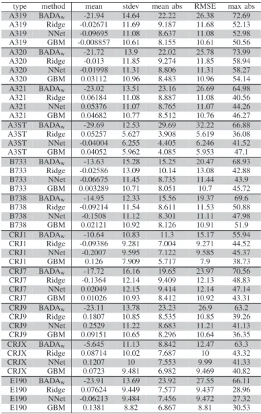
The results obtained with the Machine Learning algorithms are reported in Table VI. In this table we compare the pre-dicted distance to the observed distance Sdesc. We have tested

different methods: a ridge regression (Ridge), a neural net-work (NNet) and a gradient boosting machine (GBM). These

Figure 2: Cross-validation for model assessment, with an embedded cross-validation for hyperparameter tuning.

methods are compared with the distance dBADAw predicted by BADA. To compute this BADA prediction, the reference parameters are used concerning the mass, the descent speed profile and the aerodynamic configuration. The lateral intent and the weather are assumed to be known. Thus, we used the track angle, bank angle, wind and temperature computed from the Mode-S data. This is the baseline method.

type method mean stdev mean abs RMSE max abs A319 BADAw -21.94 14.64 22.22 26.38 72.69 A319 Ridge -0.02671 11.69 9.187 11.68 52.13 A319 NNet -0.09695 11.08 8.637 11.08 52.98 A319 GBM -0.008857 10.61 8.155 10.61 50.56 A320 BADAw -21.72 13.9 22.02 25.78 73.99 A320 Ridge -0.013 11.85 9.274 11.85 58.94 A320 NNet -0.01998 11.31 8.806 11.31 58.27 A320 GBM 0.03112 10.96 8.483 10.96 54.14 A321 BADAw -23.02 13.51 23.16 26.69 64.98 A321 Ridge 0.06184 11.08 8.887 11.08 40.56 A321 NNet 0.05376 11.07 8.765 11.07 44.26 A321 GBM 0.04682 10.77 8.512 10.76 46.27 A3ST BADAw -29.69 12.53 29.69 32.22 66.88 A3ST Ridge 0.05257 5.627 3.908 5.619 36.08 A3ST NNet -0.04004 6.255 4.405 6.246 41.52 A3ST GBM 0.04052 5.962 4.085 5.953 47.1 B733 BADAw -13.63 15.28 15.25 20.47 68.93 B733 Ridge -0.02586 13.09 10.14 13.08 42.88 B733 NNet -0.06675 11.45 8.735 11.44 43.9 B733 GBM 0.003289 10.71 8.051 10.7 45.72 B738 BADAw -14.95 12.33 15.56 19.37 69.6 B738 Ridge -0.09214 11.54 8.611 11.53 50.88 B738 NNet -0.1508 11.12 8.301 11.11 47.98 B738 GBM 0.02121 10.92 8.126 10.91 51.9 CRJ1 BADAw -10.64 10.83 11.3 15.17 55.94 CRJ1 Ridge -0.09386 9.281 7.004 9.271 44.52 CRJ1 NNet -0.2007 9.595 7.122 9.585 45.37 CRJ1 GBM 0.126 7.909 5.717 7.9 38.73 CRJ7 BADAw -17.72 16.16 19.65 23.97 70.56 CRJ7 Ridge -0.1364 12.14 9.409 12.13 48.83 CRJ7 NNet 0.02049 12.15 9.414 12.14 47.14 CRJ7 GBM 0.01026 10.93 8.412 10.92 43.31 CRJ9 BADAw -23.11 13.78 23.23 26.9 63.2 CRJ9 Ridge 0.1807 10.85 8.535 10.85 39.26 CRJ9 NNet 0.2529 11.22 8.683 11.21 41.13 CRJ9 GBM 0.09151 10.65 8.296 10.64 36.35 CRJX BADAw -5.645 11.13 8.842 12.47 63.3 CRJX Ridge 0.08714 10.02 7.687 10 43.32 CRJX NNet 0.1207 10 7.553 9.99 41.33 CRJX GBM 0.0723 9.481 6.982 9.469 40.82 E190 BADAw -23.91 13.69 23.92 27.55 66.11 E190 Ridge 0.07624 9.449 7.577 9.437 28.96 E190 NNet -0.06213 9.484 7.456 9.472 27.32 E190 GBM 0.1381 8.82 6.867 8.81 30.53

Table VI: These statistics, in nautical miles, are computed on the predicted distance minus the observed distance.

The Machine Learning methods are compared with the baseline BADAw. Among the Machine Learning methods, the

Ridge method is the less accurate one. Over the 11 aircraft types, we observe a reduction of the RMSE of 50 %, ranging from 20 % to 83 % when using the ridge regression. Using NNet, the benefit is even higher with an average reduction of 51 %. The best results are obtained with GBM with an average reduction of 55 %. For each aircraft types, a Wilcoxon signed-rank test3 _{was performed. Using a directional test, the null}

hypothesis is that most of the time the squared error obtained using Ridge is inferior to the one obtained using GBM. The null hypothesis is rejected when p-value≤ 0.01. In our results, the null hypothesis was not rejected only for the A3ST, B738 and CRJ9. Concerning the other aircraft types, this suggests that GBM is more accurate than Ridge.

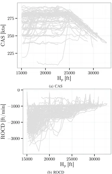
In terms of percentage, the Machine Learning methods give almost the same reduction. This is because the BADA model, i.e. the baseline, performs poorly with the reference parameters. However, in terms of nautical miles, the use of GBM over Ridge reduces further the RMSE by almost 1 NM. Concerning the A3ST, the RMSE obtained with the Machine Learning method is particularly low. This aircraft type is used by Airbus to carry aircraft parts. In our data, the A3ST follows always the same CAS/Mach speed profile during the descent. Also, the A3ST follows constant ROCD segments during the descent. Figure 3 illustrates these assertions. As a consequence, at a given altitude the ratio between the speed and the ROCD is similar for all the A3ST flights. Now, the integral of this ratio between H_pEODand H_pTODis the distance flown in the air. Thus, for a given H_pTOD and H_pEOD, all the A3ST have barely the same Sdesc.

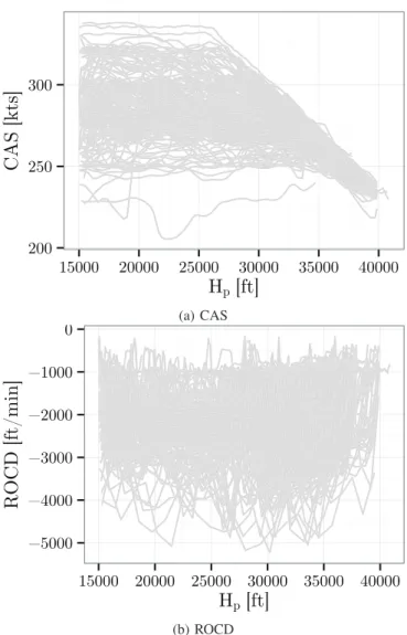
Concerning the other aircraft types, as depicted by Figure 4 for the B738, they follow several different CAS/Mach speed profiles and many aircraft do not follow a constant ROCD profile. As a result, Sdesc is more difficult to predict for these

aircraft types.

CONCLUSION

To conclude, let us summarize our approach and findings, before giving a few perspectives on future works. In this article we have described a way to predict the descent length above FL150. Using Machine Learning and a set of examples, we have built models predicting this descent length. Using real Mode-S radar, this approach has been tested on 11 different aircraft types. In order to evaluate the accuracy of the Machine Learning methods, a cross-validation was used.

When compared with the reference descent length predic-tion provided by BADA, the RMSE on the descent length is reduced, on average, by 55 % using GBM, a Machine Learning method.

In future works, we plan to predict where the descent begins along the planned route. For CDR applications, we also have to predict the positions of the aircraft during the descent. This might be done by using Machine Learning in order to predict the missing BADA parameters such as the mass and the speed/ROCD/thrust setting intent.

3_{We have used the wilcox.test provided by the R environnment, with}

the paired option.

225 250 275 15000 20000 25000 30000

Hp [ft]

C

AS [kts]

Hp [ft]

R

O

C

D

[ft/min]

Figure 3: This figure displays the CAS and the ROCD as a function of Hpfor the A3ST.

REFERENCES

[1] N. Durand, J.M. Alliot, and G. Granger. A statistical analysis of the influence of vertical and ground speed errors on conflict probe. In

Proceedings of ATM2001, 2001.

[2] X. Prats, V. Puig, J. Quevedo, and F. Nejjari. Multi-objective optimi-sation for aircraft departure trajectories minimising noise annoyance.

Transportation Research Part C, 18(6):975–989, 2010.

[3] G. Chaloulos, E. Crück, and J. Lygeros. A simulation based study of subliminal control for air traffic management. Transportation Research

Part C, 18(6):963–974, 2010.

[4] James K Kuchar and Lee C Yang. A review of conflict detection and resolution modeling methods. Intelligent Transportation Systems, IEEE

Transactions on, 1(4):179–189, 2000.

[5] Lucia Pallottino, Eric M Feron, and Antonio Bicchi. Conflict resolution problems for air traffic management systems solved with mixed integer programming. Intelligent Transportation Systems, IEEE Transactions

on, 3(1):3–11, 2002.

[6] J. M. Alliot, Hervé Gruber, and Marc Schoenauer. Genetic algorithms for solving ATC conflicts. In Proceedings of the Ninth Conference on

Artificial Intelligence Application. IEEE, 1992.

[7] N. Durand, J.M. Alliot, and J. Noailles. Automatic aircraft conflict resolution using genetic algorithms. In Proceedings of the Symposium

on Applied Computing, Philadelphia. ACM, 1996.

[8] Nicolas Durand and Jean-Marc Alliot. Ant colony optimization for air traffic conflict resolution. In 8th USA/Europe Air Traffic Management

200 250 300 15000 20000 25000 30000 35000 40000

Hp [ft]

C

AS [kts]

Hp [ft]

R

O

C

D

[ft/min]

Figure 4: This figure displays the CAS and the ROCD as a function of Hp for the B738.

[9] C. Vanaret, D. Gianazza, N. Durand, and J.B. Gotteland. Benchmarking conflict resolution algorithms. In International Conference on Research

in Air Transportation (ICRAT), Berkeley, California, 22/05/12-25/05/12,

page (on line), http://www.icrat.org, may 2012. ICRAT.

[10] R. Alligier, D. Gianazza, and N. Durand. Machine learning and mass estimation methods for ground-based aircraft climb prediction.

Intelligent Transportation Systems, IEEE Transactions on, 16(6):3138–

3149, Dec 2015.

[11] R. Alligier, D. Gianazza, and N. Durand. Machine learning applied to airspeed prediction during climb. In Proceedings of the 11th USA/Europe

Air Traffic Management R & D Seminar, 2015.

[12] Steven M Green and Robert Vivona. Field evaluation of descent advisor trajectory prediction accuracy. In AIAA Guidance, Navigation and

Control Conference, volume 1, 1996.

[13] Steven Green, Robert Vivona, Michael Grace, and Tsung-Chou Fang. Field evaluation of descent advisor trajectory prediction accuracy for en route clearance advisories. In AIAA98-4479, AIAA GNC

Confer-ence.(August 1998), 1998.

[14] ADAPT2. aircraft data aiming at predicting the trajectory. data analysis report. Technical report, EUROCONTROL Experimental Center, 2009. [15] Laurel Stell. Predictability of top of descent location for operational idle-thrust descents. In 10th AIAA Aviation Technology, Integration, and

Operations Conference, Fort Worth, TX, 2010.

[16] Laurel Stell. Prediction of top of descent location for idle-thrust descents. In 9th USA/Europe Air Traffic Management R&D Seminar,

Berlin, Germany, 2011.

[17] L. Stell, J. Bronsvoort, and G. McDonald. Regression analysis of top

USA/Europe Air Traffic Management R & D Seminar, 2013.

[18] EUROCONTROL Experimental Centre. User manual for base of aircarft data (bada) rev.3.13. Technical report, EUROCONTROL, 2015. [19] T. Hastie, R. Tibshirani, and J. H. Friedman. The Elements of Statistical

Learning. Springer Series in Statistics. Springer New York Inc., New

York, NY, USA, 2001.

[20] C. M Bishop. Pattern recognition and machine learning, volume 1. springer New York, 2006.

[21] Vladimir N. Vapnik and Alexey Ya. Chervonenkis. The necessary and sufficient conditions for consistency of the method of empirical risk minimization. Pattern Recogn. Image Anal., 1(3):284–305, 1991. [22] Vladimir N. Vapnik. The nature of statistical learning theory.

Springer-Verlag New York, Inc., New York, NY, USA, 1995.

[23] Avrim Blum, Adam Kalai, and John Langford. Beating the hold-out: Bounds for k-fold and progressive cross-validation. In Proceedings of

the twelfth annual conference on Computational learning theory, pages

203–208. ACM, 1999.

[24] R. Kohavi. A study of cross-validation and bootstrap for accuracy estimation and model selection. pages 1137–1143. Morgan Kaufmann, 1995.

[25] J. Fox. Applied regression analysis, linear models, and related methods. Sage Publications, Inc, 1997.

[26] C. R. Rao and H. Toutenburg. Linear Models: Least Squares and

Alternatives (Springer Series in Statistics). Springer, July 1999.

[27] Arthur E. Hoerl and Robert W. Kennard. Ridge regression: Biased estimation for nonorthogonal problems. Technometrics, 12(1):55–67, 1970.

[28] M. I. Jordan and C. Bishop. Neural Networks. CRC Press, 1997. [29] C. M. Bishop. Neural networks for pattern recognition. Oxford

University Press, 1996. ISBN: 0-198-53864-2.

[30] B. D. Ripley. Pattern recognition and neural networks. Cambridge University Press, 1996. ISBN: 0-521-46086-7.

[31] Jerome H. Friedman. Stochastic gradient boosting. Computational

Statistics Data Analysis, 38(4):367 – 378, 2002.

[32] J. H. Friedman. Greedy function approximation: A gradient boosting machine. Annals of Statistics, 29:1189–1232, 2000.

[33] L. Breiman, J. H. Friedman, R. A. Olshen, and C. J. Stone.

Classifi-cation and Regression Trees. Statistics/Probability Series. Wadsworth

Publishing Company, Belmont, California, U.S.A., 1984.

[34] G. Ridgeway. Generalized boosted models: A guide to the gbm package.

Update, 1:1, 2007.

BIOGRAPHIES

Richard Alligier received his Ph.D. (2014) degree in Com-puter Science from the "Institut National Polytechnique de Toulouse" (INPT), his engineers degrees (IEEAC, 2010) from the french university of civil aviation (ENAC) and his M.Sc. (2010) in computer science from the University of Toulouse. He is currently assistant professor at the ENAC in Toulouse, France.

David Gianazza received his two engineer degrees (1986, 1996) from the french university of civil aviation (ENAC) and his M.Sc. (1996) and Ph.D. (2004) in Computer Science from the "Institut National Polytechnique de Toulouse" (INPT). He has held various positions in the french civil aviation administration, successively as an engineer in ATC operations, technical manager, and researcher. He is currently associate professor at the ENAC, Toulouse.

Nicolas Durand graduated from the Ecole polytechnique de Paris in 1990 and the Ecole Nationale de l’Aviation Civile (ENAC) in 1992. He has been a design engineer at the Centre d’Etudes de la Navigation Aérienne (then DSNA/DTI R&D) since 1992, holds a Ph.D. in Computer Science (1996) and got his HDR (french equivalent of tenure) in 2004. He is currently professor at the ENAC/MAIAA lab.