To link to this article : DOI :
10.1109/JSTARS.2016.2569162
URL :
https://doi.org/10.1109/JSTARS.2016.2569162
To cite this version :
Campos-Taberner, Manuel and Romero-Soriano,
Adriana and Gatta, Carlo and Camps-Valls, Gustau and Lagrange,
Adrien and Le Saux, Bertrand and Beaupère, Anne and Boulch,
Alexandre and Chan-Hon-Tong, Adrien and Herbin, Stéphane and
Randrianarivo, Hicham and Ferecatu, Marin and Shimoni, Michal and
Moser, Gabriele and Tuia, Devis Processing of Extremely
High-Resolution LiDAR and RGB Data: Outcome of the 2015 IEEE GRSS
Data Fusion Contest - Part A: 2-D Contest. (2016) IEEE Journal of
Selected Topics in Applied Earth Observations and Remote Sensing,
vol. 9 (n° 12). pp. 5547-5559. ISSN 1939-1404
O
pen
A
rchive
T
OULOUSE
A
rchive
O
uverte (
OATAO
)
OATAO is an open access repository that collects the work of Toulouse researchers and
makes it freely available over the web where possible.
This is an author-deposited version published in :
http://oatao.univ-toulouse.fr/
Eprints ID : 18877
Any correspondence concerning this service should be sent to the repository
administrator:
[email protected]
Processing of Extremely High-Resolution LiDAR
and RGB Data: Outcome of the 2015 IEEE GRSS
Data Fusion Contest–Part A: 2-D Contest
Manuel Campos-Taberner, Adriana Romero-Soriano, Carlo Gatta, Gustau Camps-Valls, Senior Member, IEEE,
Adrien Lagrange, Bertrand Le Saux, Anne Beaup`ere, Alexandre Boulch, Adrien Chan-Hon-Tong, Stephane Herbin,
Hicham Randrianarivo, Marin Ferecatu, Michal Shimoni, Member, IEEE, Gabriele Moser, Senior Member, IEEE,
and Devis Tuia, Senior Member, IEEE
Abstract—In this paper, we discuss the scientific outcomes of the
2015 data fusion contest organized by the Image Analysis and Data Fusion Technical Committee (IADF TC) of the IEEE Geoscience and Remote Sensing Society (IEEE GRSS). As for previous years, the IADF TC organized a data fusion contest aiming at fostering new ideas and solutions for multisource studies. The 2015 edi-tion of the contest proposed a multiresoluedi-tion and multisensorial challenge involving extremely high-resolution RGB images and a three-dimensional (3-D) LiDAR point cloud. The competition was framed in two parallel tracks, considering 2-D and 3-D products, respectively. In this paper, we discuss the scientific results obtained by the winners of the 2-D contest, which studied either the comple-mentarity of RGB and LiDAR with deep neural networks (winning team) or provided a comprehensive benchmarking evaluation of new classification strategies for extremely high-resolution multi-modal data (runner-up team). The data and the previously
undis-The work of A. Romero was supported by an APIF-UB grant. undis-The work of C. Gatta was supported by MICINN under a Ramon y Cajal Fellowship. The work of M. Campos was supported by the European Union Seventh Framework Program FP7/2007-2013 under Grant 606983, and the LSA SAF (EUMETSAT) project. The work of G. Camps-Valls was supported by the European Research Council funding of the ERC-CoG-2014 SEDAL Consolidator Grant 647423, and the Spanish Ministry of Economy and Competitiveness for the funding through the Project LIFE-VISION TIN2012-38102-C03-01. The work of D. Tuia was supported by the Swiss National Science Foundation under Grant PP00P2-150593. (Corresponding author: Devis Tuia.)
M. Campos-Taberner and G. Camps-Valls are with the Universitat de Val`encia, Valencia 46010, Spain (e-mail: [email protected]; gcamps@ uv.es).
A. Romero-Soriano is with the Universitat de Barcelona, Barcelona 08007 Spain (e-mail: [email protected]).
C. Gatta is with the Universitat Aut`onoma de Barcelona, Barcelona 08193 Spain (e-mail: [email protected]).
A. Lagrange, B. Le Saux, A. Beaup´ere, A. Boulch, A. Chan-Hon-Tong, S. Herbin, and H. Randrianarivo are with the Office National d’Etudes et de Recherches A´erospatiales—The French Aerospace Lab, Palaiseau 91123, France (e-mail: [email protected]; [email protected]; [email protected]; [email protected]; adrien.chan_hon_tong@ onera.fr; [email protected]; [email protected]).
M. Ferecatu is with the Conservatoire National des Arts et Metiers – Cedric, Paris 75141, France (e-mail: [email protected]).
M. Shimoni is with the Signal and Image Centre, Department of Electrical Engineering, Royal Military Academy, Brussels 1000, Belgium (e-mail: [email protected]).
G. Moser is with the Department of Electrical, Electronic, Telecommunica-tions Engineering and Naval Architecture, University of Genoa, Genoa 16145, Italy (e-mail: [email protected]).
D. Tuia is with the Department of Geography, University of Zurich, Zurich 8057, Switzerland (e-mail: [email protected]).
closed ground truth will remain available for the community and can be obtained at http://www.grss-ieee.org/community/technical-committees/data-fusion/2015-ieee-grss-data-fusion-contest/. The 3-D part of the contest is discussed in the Part-B paper [1].
Index Terms—Deep neural networks, extremely high spatial
resolution, image analysis and data fusion (IADF), landcover classification, LiDAR, multiresolution-, multisource-, multimodal-data fusion.
I. INTRODUCTION TO THE2015 CONTEST
T
HE current development of Earth observation (EO) technologies, encompassing satellite missions, airborne acquisitions, drones, and unmanned aerial vehicles (UAV) is providing remote sensing scientists and practitioners with more and more opportunities to collect data of the Earth’s surface for multiple global, regional, and local applications. These data can differ substantially in their physical natures (e.g., opti-cal, thermal, radar, or laser observations), spatial resolutions (from a few centimeters to some kilometers using aerial and geostationary platforms, respectively), spectral resolutions (from panchromatic to hyperspectral imagery), and temporal resolutions (from a few minutes with geostationary systems to hours or days with constellations of near-polar satellites, and to on-demand acquisition with UAVs) [2].In this framework, the capability to jointly benefit from those images critically depends on the development of accurate data fusion algorithms that effectively model the complementary information conveyed by distinct data sources [3]–[5]. Mul-tisensor [6]–[8], multitemporal [9]–[11], and multiresolution [12]–[14] fusion techniques for remote sensing data have been researched for long, and are currently more and more relevant as they need to keep pace with the opportunities provided by these new data and the methodological challenges they raise [5]. It is in this framework that the IEEE Geoscience and Remote Sensing Society (IEEE GRSS) Image Analysis and Data Fusion Technical Committee (IADF TC1) organizes an annual Data Fusion Contest, in which a dataset is released free of charge to the international community along with a data fusion competi-tion [7], [9], [12], [15]–[18]. This paper is the first of a two-part manuscript that aims at presenting and critically discussing the scientific outcomes of the 2015 edition of the Contest.
The 2015 Contest released to the international community of remote sensing an image dataset involving multiresolution
and multisensor imagery, extremely high spatial resolutions, and three-dimensional (3-D) information. The dataset was com-posed of an RGB orthophoto and of a LiDAR point cloud ac-quired over an urban and harbor area in Zeebruges, Belgium (see Section II).
Given the relevance of this dataset for the modeling and ex-traction of both 2-D and 3-D thematic results, the Contest was framed as two independent and parallel competitions. The 2-D Contest was focused on multisource fusion for the generation of 2-D products at extremely high spatial resolution. The 3-D Contest explored the synergistic use of 3-D point cloud and 2-D RGB data for 3-D analysis.
In either case, participating teams submitted original open-topic manuscripts summarizing their idea and the analysis on the dataset provided. All submissions were evaluated and ranked by an Award Committee, composed of the organizers of the Contest and of several present and past Chairs and Cochairs of IADF TC, on the basis of scientific contribution, methodological ap-proaches, experimental discussion, and quality of presentation. Consistently with the two-track structure, four papers were awarded (two per track) and were presented during the IGARSS 2015 conference in Milan. According to the different applicative and methodological problems addressed by the two tracks, their outcomes are now discussed in two articles, a Part A (this paper) on the 2-D contest and a Part B [1] on the 3-D Contest. Each paper is coauthored by the winning teams of each competition, along with the Contest organizers. For the 2015 edition of the data fusion contest, track 2-D, the papers awarded were:
1) 1st Place: “Shared feature representations of LiDAR and optical images: Trading sparsity for semantic discrimi-nation,” by Manuel Campos-Taberner, Adriana Romero,
Carlo Gatta, and Gustau Camps-Vallsfrom the Univer-sity of Val`encia, the Universitat de Barcelona, and the Universitat Aut`onoma de Barcelona (Spain) [19]. 2) 2nd Place: “Benchmarking classification of
Earth-observation data: From learning explicit features to con-volutional networks” by Adrien Lagrange, Bertrand Le
Saux, Anne Beaupere, Alexandre Boulch, Adrien Chan-Hon-Tong, Stephane Herbin, Hicham Randrianarivo, and Marin Ferecatu from the Onera Paris and the CNAM (France) [20].
The remainder of Part A is as follows: Section II provides a detailed description of the dataset. Then, the overall set of sub-missions is presented in Section III. The approaches proposed by the first- and second-ranking teams are presented in Sections IV and V, respectively. Finally, a discussion of these two ap-proaches is presented in Section VI. Overall conclusion on the 2015 Data Fusion Contest can be found in Part B [1].
II. DATASET
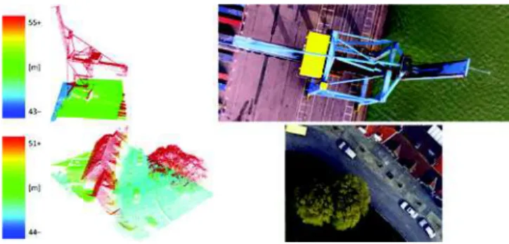
The 2015 Contest involved two datasets acquired simultane-ously by passive and active sensors (see Fig. 1). Both datasets were acquired on March 13, 2011, using an airborne platform flying at an altitude of 300 m over the harbor area of Zeebruges, Belgium (51.33◦N,3.20◦E). The Department of
Communica-tion, InformaCommunica-tion, Systems and Sensors (CISS) of the Belgian
Fig. 1. Examples of details of the3-D point cloud along with the correspond-ing portions of the orthophoto data. RGB details are oriented consistently with Fig. 2. Point cloud details have been oriented manually to enhance their visual display. Color bars indicate height in the point clouds.
Royal Military Academy (RMA) provided the dataset and evaluated its accuracy while the service provider acquired and preprocessed the data.
The passive dataset is a 5-cm-resolution RGB orthophoto acquired in the visible wavelength range (see Fig. 2). The active source is a LiDAR system that acquired the data using repe-tition rate, angle, and frequency of 125 kHz, 20◦, and 49 Hz,
respectively. The laser repetition rate refers to the number of times per second a scanning device samples its field of view, the angle indicates the field of view, and the frequency refers to the number of emitted pulses per second. For obtaining a digital surface model (DSM) with a point spacing of 10 cm, the area of interest was scanned several times in different directions with a high-density point cloud rate of 65 pts/m2. The scanning mode was “last, first, and intermediate.” Multiple returns are capable of detecting the elevations of several objects within the laser footprint of an outgoing laser pulse. The first returned laser pulse is the most significant return and is generally associated with the highest feature in the landscape like a treetop or the top of a building. The intermediate returns, in general, are used for vegetation structure, and the last return for bare-Earth terrain models. This scan mode was used to filter the cloud points and to facilitate the creation of the DSM. Indirect georeferencing using a large set of well-distributed ground control points was selected as the method for coregistration due to its accuracy and robustness against interior orientation parameters biases [21]. This procedure completed the georeferencing obtained using the LiDAR system’s GPS and the inertial navigation system on board the aircraft. Both the raw3-D point cloud (see Fig. 1) and the DSM (see Fig. 3) were distributed to the community.
This dataset corresponded to the finest spatial resolution ad-dressed so far by the IEEE GRSS Data Fusion Contests, and made for a very challenging image analysis and fusion com-petition. The large data volume was possibly time consuming and expensive to process, but the highly detailed information allowed the users to provide results resembling a real-world situation. Nevertheless, this rich dataset demanded the innova-tion and the adaptainnova-tion of many numerical tools for registrainnova-tion and for obtaining the relation between the target geometry, the measured scattering, and the corresponding height and target-scattering properties in the2-D and the 3-D dimensions.
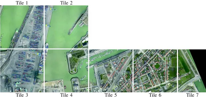
Fig. 2. Seven tiles of the RGB dataset (RGB) of the Data Fusion Contest 2015. The data can be freely downloaded on http://www.grss-ieee.org/community/technical-committees/data-fusion/2015-ieee-grss-data-fusion-contest/
Fig. 3. Seven tiles of the DSM issued from the LiDAR point cloud of the Data Fusion Contest 2015. The data can be freely downloaded on http://www.grss-ieee.org/community/technical-committees/data-fusion/2015-ieee-grss-data-fusion-contest/
III. DISCUSSION OF THE2-D CONTEST: THESUBMISSIONS
Twenty papers were submitted to the 2-D contest. We ob-served a large variety in the topics considered in the manuscripts, as well as in the processing approaches presented. Below we discuss these two aspects separately.
A. Addressed Topics
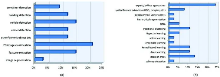
Fig. 4(a) summarizes the topics tackled by the participants. Even though general 2-D classification was the most represented topic, several teams developed specific strategies for the data at hand. We observed a wide, almost uniform, distribution of the topics, ranging from traditional image processing tasks (2-D image classification, feature extraction) to image-specific
detection tasks (container, vessels, or vehicle detection). On one hand, the large number of submissions on 2-D classification was an expected result because this topic is a customary one in the tradition of Data Fusion Contests and is of great prominence in the IADF TC community. On the other hand, the variety of addressed topics was also an interesting outcome and confirmed the choice of an open-topic competition with the considered extremely high-resolution dataset.
B. Proposed Processing Approaches
Fig. 4(b) details the spread of the processing approaches proposed by the participants. Many approaches were based on expert or ad hoc systems with manual thresholding and
Fig. 4. Summary of the 20 submissions to the 2-D contest by topics (a) and approaches considered (b).
hand-crafted task-specific features. These approaches were characterized by relatively simple and highly customized de-cision rules aimed at given thematic classes or target objects and applied to case-specific elevation, vegetation index, shape, etc., features. From the viewpoint of applications, the large num-ber of submissions of this category matches the prominence of classification and object detection among the addressed prob-lems and the focus on the extraction of specific characteristics of the imaged urban and port area. From a methodological per-spective, these techniques privileged the precision of the results and focused on the best parametrization of simple approaches to solve specialized detection or discrimination tasks.
A second group of submissions regarded the proposal and validation of novel methods to use the new type of data released. In this respect, several learning approaches, en-compassing supervised Bayesian, kernel, deep, and ensemble methods, unsupervised clustering and segmentation, and semi-interactive active learning were considered. This category of submissions is consistent with the aforementioned focus on classification problems and with the relevance of the related methodologies within the IADF TC community. Nonetheless, it is worth noting that the submitted algorithms ranged from rather consolidated approaches to recent topical solutions based on kernel methods and deep neural networks. These solutions were proposed to investigate the nature and complementarity of the data and perform classification or detection. In this case, the focus was in the study of the adequateness of the approach for this type of data in general purpose classification/clustering tasks. Furthermore, most of the aforementioned learning methods were combined with spatial modeling and feature ex-traction techniques, including histograms of oriented gradients (HOGs), mathematical morphology, region-based or object-based processing, and texture analysis. This was an expected outcome due to extremely high spatial resolution of the input data.
A third and last group can be mentioned, that includes uncon-ventional strategies, at least with respect to the past Data Fusion Contests: Solutions based on agent modeling or saliency detec-tion, which are relatively popular in other research areas (e.g.,
financial modeling and visual color analysis) but not frequently explored in remote sensing, were also received. These submis-sions suggested that new avenues were also explored beyond the two former (and more traditional) ones.
IV. SHAREDFEATUREREPRESENTATIONS OFLIDARAND
OPTICALIMAGES: TRADINGSPARSITY FORSEMANTIC
DISCRIMINATION
This section presents the results obtained by the winning team of the 2-D contest and is an extension of [19]. The work fo-cuses on an indirect approach via unsupervised spatial–spectral feature extraction with the aim of studying the level of com-plementary information conveyed by extremely high resolution LiDAR and optical images. For this purpose, the study used an unsupervised convolutional neural network (CNN) [22] trained to enforce both population (PS) and lifetime sparsity (LS) in the (joint, shared) feature representation. The obtained results re-vealed that the RGB+LiDAR representation is no longer sparse, and the derived basis functions merge color and elevation yield-ing a set of more expressive colored edge filters. The joint feature representation is also more discriminative when used for clus-tering and topological data visualization.
A. Motivation
Image fusion of optical and LiDAR images is currently a successful and active field [23]–[28]. Intuition and physics tell us that both modalities represent objects in the scenes in different
semanticways: color versus altitude, or passive radiance versus active return intensity. But, is there a fundamental justification for this in statistical terms?
Answering such question directly would imply measuring mutual information between data modalities. However, the involved random variables (i.e., RGB and LiDAR imagery) are multidimensional, they do have spatial structure, and do reveal distinctive spatial–spectral feature relations. An indirect pathway was followed here: To analyze spatial– spectral feature representations with CNNs using RGB, Li-DAR, and the RGB+LiDAR shared representation. Such feature
representations were studied in terms of sparsity, compactness, topological visualization, and discrimination capabilities.
The statistical properties of very high-resolution (VHR) and multispectral images raise important difficulties for automatic analysis, because of the high spatial and spectral redundancy, and their potentially nonlinear nature.2 Beyond these well-known data characteristics, we should highlight that spatial and spectral redundancy also suggest that the acquired signal may be better described in sparse representation spaces, as recently reported in [31] and [30]. Seeking for sparsity may in turn be beneficial to deal with the increasing amount of data due to im-provements in spatial resolution. Learning expressive spatial–
spectral features from images in an efficient way is, thus, of paramount relevance. Moreover, learning such features in an
unsupervisedfashion is an even more important issue.
In recent years, dictionary learning has emerged as an effi-cient way to learn sparse image features in unsupervised set-tings, which are eventually used for image classification and object recognition: Discriminative dictionaries have been pro-posed for spatial–spectral sparse-representation for image clas-sification [32], [33], sparse bag-of-words codes for automatic target detection [34], and unsupervised learning of sparse fea-tures for aerial image classification [35]. Most of these methods describe the input images in sparse representation spaces but do not take advantage of the highly nonlinear nature of CNNs archi-tectures. In this study, the use of unsupervised feature learning with CNNs was introduced with the goal of studying the statis-tical properties of joint RGB+LiDAR representation spaces.
B. Unsupervised Feature Learning With Convolutional Networks
CNNs ([36], [37]) are nonlinear models that capture spatial– local interactions and provide hierarchical representations of the input data. CNNs consist of successive representation layers stacked together, such that the output of a layer is used as input to the following layer. In our case, the input to the first layer is the RGB and/or LiDAR imagery. Each layer of a CNN is pa-rameterized by a set of learnable weights and biases, where the weights constitute a set of linear filters. The output of each layer is obtained by 1) convolving the input with the linear filters and adding a bias term to allow shifting the obtained results; 2) ap-plying a point-wise nonlinearity, e.g., the logistic function; and 3) performing a pooling operation, e.g., a nonoverlapping2 × 2 sliding window computing the maximum of its input (called
max-pooling). The rationale of these three parts is 1) to provide a simple local feature extraction; 2) to modify the result in a nonlinear way to allow the CNN architecture to learn nonlinear representations of the data; and 3) to reduce the computational cost and provide a certain local translational invariance.
Although most of the recent success of CNNs relies on train-ing them in a supervised fashion [36], [37]; significant effort has been devoted to propose unsupervised algorithms to extract
2Factors such as multiscattering in the acquisition process, heterogeneities at subpixel level, as well as atmospheric and geometric distortions lead to distinct nonlinear feature relations, since pixels lie in high-dimensional curved manifolds [29], [30].
general meaningful feature representations. A successful way to train CNN architectures in an unsupervised way is by means of greedy layer-wise pretraining [38], [39], where each layer of the network is trained in isolation, following an unsupervised cri-terion. After pretraining, the weights and biases of the network are set to a potentially good local minima. Many state-of-the-art unsupervised criteria follow sparsity constraints [40]. Sparsity is usually defined in terms of population sparsity (PS) and/or
lifetime sparsity (LS). PS ensures that only a small subset of features are active per sample, providing a simple interpretation of the data. LS ensures that each feature is active for a small amount of samples, avoiding the presence of “dead” features, i.e., those features that do not activate much.
Among state-of-the-art unsupervised methods seeking spar-sity, orthogonal matching pursuit (OMP-k) [40] trains a set of filters by iteratively selecting a feature to be made nonzero with the objective of minimizing the residual reconstruction er-ror. This is done until at most k features have been selected, thus, achieving a sparse representation of the data in terms of PS. Sparse autoencoders train the filters by minimizing the re-construction error while ensuring similar activation statistics through all training samples among all outputs, thus, achieving a sparse representation of the data in terms of LS.
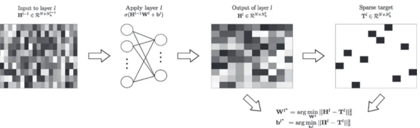
In this paper, we use the enforcing population and lifetime sparsity (EPLS) algorithm [22] to train convolutional networks. The algorithm iteratively builds a sparse target and optimizes for that specific sparse target to learn the filters of one layer. The sparse target is designed such that it represents each sample with one “hot code” and uniformly distributes the feature activations over the samples, achieving both PS and LS in the feature rep-resentation. Fig. 5 summarizes the steps of the method in [22]. Essentially, given a matrix of input patches to train layerl, Hl−1,
we need to: 1) compute the output of the patches Hlby applying the learned weights and biases to the input, and subsequently the nonlinearity; 2) call the EPLS algorithm to generate a sparse target Tl
from the output of the layer, such that it ensures PS and LS; and 3) optimize the parameters of the layer (weights and biases) by minimizing theL2 norm of the difference between
the layer’s output and the EPLS sparse target θl∗= arg min
θl ||H
l− Tl||2
2. (1)
The optimization is performed by means of an out-of-the-box minibatch stochastic gradient descent with adaptive learning rates [41]. From now on, we use the superscriptb to refer to the data related to a minibatch, e.g., the output of a layer Hl∈ RN ×Nhl will now be Hl,b∈ RNb×Nhl, where Nb < N is the
number of patches in a minibatch.
Even though the EPLS algorithm can be effectively used in combination with deep CNN architectures, as in [42], we here restrict ourselves to single layer CNNs for the sake of inter-pretability. The CNN training by means of EPLS is computa-tionally very efficient and leads to sparse representations of the input data. Here, we train single layer CNNs on RGB, LiDAR, and RGB+LiDAR input spaces and analyze the resulting hid-den and shared representations, see Fig. 6. Note that the shared
Fig. 5. Illustration of how EPLS generates the output target matrix. The processing flow in the proposed algorithm is as follows: The outputs of a CNN layer is Hl= σ(Hl −1Wl+ bl), where Hl −1is the input feature map to thelth layer; θl= {Wl, bl} is the set of learnable parameters (weights and biases) of the layer, andσ(·) is the point-wise nonlinearity. The input of the first layer is the input data (e.g., a multispectral image), i.e., H0= I, where I ∈ RN ×N0
h is the input image,N is the sample size (patch pixels), and N0
h is the number of spectral channels (bands). The output of the layerl is then sparse-coded via the (unsupervised) EPLS algorithm to yield a sparse target, and theL2norm of the difference between the layer’s output and the EPLS sparse target computed, and used to fit network filters.
Fig. 6. Considered independent (a) RGB and (b) LiDAR representations, along with the (c) shared RGB+LiDAR representation.
RGB+LiDAR representation is made of nonlinear spatial and spectral combinations of input RGB and LiDAR features.
C. Results and Discussion
In this section, we analyze the information content captured by a CNN trained to enforce sparsity in the three scenarios: RGB, LiDAR, and joint RGB+LiDAR. We report on: 1) the LS and PS scores, analyzed as a measure of compactness of the representations; 2) the learned representations, visualized in a topological space; 3) the discriminative power of the extracted features when used for image segmentation.
1) Experimental Setup: We consider tile #3 (see Figs. 2 and 3), for which 100 000 image patches of size 10 × 10 were extracted. A total number of 30 000 images patches were used for training the networks. In all the three situations, the CNNs were trained using a maximum ofNH = 1000 hidden
nodes. For all the architectures, several symmetric receptive fields (RFs) (of sizes3 × 3 and 5 × 5, 7 × 7, 10 × 10 pixels) were tried. The networks were trained on contrast-normalized image patches by means of EPLS [22] with logistic non-linearity. The sparse features were retrieved by applying the network parameters with natural encoding (i.e., with the lo-gistic nonlinearity) and polarity split. Polarity splitting takes into account the positive and negative components of a code (weights) and hence doubles the number of outputs and is usu-ally applied to the output layer of the network. The interested
Fig. 7. Lifetime and population sparsity for RGB, LiDAR, and RGB+LiDAR as a function of the receptive field RF (top) and the number of hidden neurons (NH, bottom).
reader may find an implementation of the EPLS algorithm in http://www.cvc.uab.es/People/aromero/EPLS.html.
2) On the Sparsity of the Learned Representations: After training the CNNs in the three situations, both the LS and the PS were studied (see Fig. 7). One can see that by adding LiDAR to RGB, LS is increased, independently of the RF (i.e., the size of the convolution window) used. Note that the lower the value of LS, the closer to the objective of maintaining similar mean activation among outputs. The learned representation is, thus, no longer sparse, which suggests that RGB and LiDAR carry orthogonal information and, thus, it is more difficult to obtain a compact representation. Similar trends were obtained when varying NH, but only for high values, say NH > 100,
which can be due to the poor representation in general obtained for low values of NH (big errors, results not shown). On the
Fig. 8. Learned bases by the convolutional net using EPLS for RGB, LiDAR, and RGB+LiDAR (top), and the corresponding topological representations via projection on the first two ISOMAP components (bottom).
contrary, by adding LiDAR to RGB, PS is reduced for any RF andNH value. The same reasoning as before holds here. PS
captures that a small subset of outputs are very active at the same time. This does not happen when merging RGB+LiDAR because these features convey complementary information and hence many features activate simultaneously.
3) On the Topology of the Learned Representations: Fig. 8 shows the bases learned by the convolutional net using EPLS for RGB, LiDAR, and RGB+LiDAR (top), and the correspond-ing topological representations via projection on the first two ISOMAP components (bottom). The neighborhood was inten-tionally fixed to c = 1 in ISOMAP’s epsilon distance for the sake of simplicity in the visualization of the representations. The EPLS algorithm applied to VHR RGB images [see Fig. 8(a)] learns not only common bases such as oriented edges/ridges in many directions and colors, but also corner detectors, tribanded colored filters, center surrounds, and Laplacian of Gaussians among others [22]. This suggests that enforcing LS helps the system to learn a set of complex and rich bases. On the other hand, the learned LiDAR bases [see Fig. 8(b)] are edge detectors related to “changes in height” of the objects, e.g., containers-versus-ground, roof-versus-ground, ground-versus-sea, roofs, train rails versus ground in the image. When com-bining RGB+LiDAR [see Fig. 8(c)], the learned bases inherit properties of both modalities, resembling altitucolored de-tectors.
For the projections onto the first two ISOMAP components, we can see that RGB bases scatter twofold [see Fig. 8(d)]: A color-predominant diagonal on top of a typical edges and triband grayscale textures. Higher frequency (both grayscale and colored) lie far from the subspace center. In the LiDAR case [see Fig. 8(e)], the scatter is much simpler: Low frequencies in the center and height edges surrounding the center of the subspace. When RGB and LiDAR are combined [see Fig. 8(f)], color and texture clusters are disentangled, but height edges become
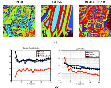
Fig. 9. (a) Clustering maps obtained usingk-means on top of the CNN fea-tures. (b) Cluster quality indices as a function of the number of clustersk.
slightly more colored, and again high-frequency patterns lie far from the mean.
4) On the Discriminative Power of the Representations: An alternative way to analyze the extracted features and their com-plementarity is to use them for clustering. The standardk-means was run on top of the extracted features for different degrees of granularity, k = 2, . . . , 20. Fig. 9(a) shows the classifica-tion maps fork = 10. It should be noted that RGB dominates many clusters in the joint/shared representation. Nevertheless, the RGB+LiDAR map shows new emerging groups of semantic clusters, e.g., harbor cranes close the sea. Some other clusters are just inherited from the individual LiDAR solution, e.g., big buildings with constant height. The quality of clustering solu-tions is a controversial issue and many techniques exist in the literature to evaluate clustering solutions. The general idea in all of them is to favor compact and distant clusters. Fig. 9(b) shows two quality indices: the Davies–Bouldin [43] and the Dunn [44] validity indices as a function ofk (similar results were obtained for theR2and the Calinski–Harabasz [45] indices, not shown).
Results suggest that the joint representation leads to similar so-lutions to those obtained with RGB alone, yet resemble more semantically expressive.
5) Discussion: The expressive power and richfulness of fea-tures extracted from RGB, LiDAR, and RGB+LiDAR were ana-lyzed using state-of-the-art unsupervised learning. In particular, this study used a recently presented unsupervised CNN that aims to learn feature representations that are sparse. This dis-tinct characteristic of the algorithm has revealed very useful in semantic segmentation of images. However, in our experi-ments, the combination of RGB and LiDAR has given rise to a feature representation that is no longer sparse according to different sparsity scores, thus, suggesting that RGB and LiDAR convey “orthogonal” and complementary pieces of informa-tion. Beyond the focus on sparsity, we also payed attention to the induced topological spaces through ISOMAP embeddings.
The analysis again revealed interesting complementarity: RGB combined with LiDAR leads to more semantic representations in which color and altitude are combined to better object de-scription. The obtained joint feature representation suggests a kind of semantic extraction. The orthogonality in information does not only come out in terms of lack of sparse solutions, but also in terms of discrimination, as it was studied through image segmentation, where more expressive and semantic maps emerge.
V. BENCHMARKINGCLASSIFICATION OFEO DATA: FROM
LEARNINGEXPLICITFEATURES TOCONVOLUTIONAL
NETWORKS
This section presents the results obtained by the runner-up team of the 2-D contest and is an extension of [20]. The paper focuses on a wide benchmarking effort of different state-of-the-art classification approaches and in the design of a fair and challenging validation setting for supervised classification at extremely high spatial resolution.
A. Motivation
The study of urban areas using EO is relevant for several ap-plications, going from urban management to flows monitoring, and in the meantime raises great challenges: Numerous and di-verse semantic classes, occlusions or bizarre geometries due to either the acquisition angle or the orthorectification. Semantic labeling consists of automatically building maps of geolocal-ized semantic classes. It evolves along with the resolution of the images and the availability of labeled data. The contribu-tion of the resolucontribu-tion is straightforward: With more details, new potential semantic classes can be distinguished in the images, from roads and urban areas to buildings and trees. Image de-scription evolved from textures to complex features that allow object modeling [46], [47]. Numerous statistical methods were developed for multiclass urban classification [48], [49]. A re-cent trend is to use very large labeled sets to train deep networks [50], for example based on convolutional networks [51].
Despite these impressive advances, semantic labeling still faces unsolved problems: Which method is best suited for a given class? Is it possible to build a classifier which is generic enough to handle a large variety of labels? Indeed, semantic classes may have really diverse structures, from large, loose areas (i.e., vegetation areas) to rigid, structured objects (such as cars, street furniture, etc.). With the advent of VHR images, the latter becomes more and more frequent.
The VHR multisensor dataset provided in the framework of the 2015 IEEE GRSS Data Fusion Contest provides us with a large variety of semantic classes. In this study, we use it as the benchmark needed by the EO community for rigorously assessing and comparing the various approaches that coex-ist. For this purpose, we built up a ground truth with eight classes (see Section V-B). We implemented and tested various approaches ranging from expert and sensor-based baselines to powerful machine-learning approaches, aiming at both pixel-wise and object-pixel-wise classification (see Section V-C). Their respective performances are then evaluated and compared (see
TABLE I
GROUNDTRUTHCLASSES FORSEMANTICLABELING(WITHCLASS
PROPORTION ANDNUMBER OFPIXELSOVER THEENTIREDATASET)
Section V-D), then showing which ones are best suited for some specific applications and which ones could be used for generic purposes.
B. Benchmark
We manually built a ground truth (see Fig. 10) with the se-mantic labels summarized in Table I. To this aim, we processed carefully the labeling following image analysis procedures and we cross validated the ground truth among different people to detect annotation errors and improve accuracy (see Fig 11 for a visual assessment). Given its geographic situation, Zeebruges provides a wide range of semantic classes of interest (in bold face in the following). Standard urban classes like buildings, vegetation (that we divided in low vegetation and trees) and
impervious surfaces (mainly roads) can be found. But the
har-bor part of the town also offers water, vessels, and industrial installations (such as cranes and containers), the latter being mainly gathered in the clutter category. Given the exceptionally good resolution, we were also able to define two object-oriented classes: cars and boats.
For the evaluation, we performed cross validation on the dataset to assess the various methods. We retained tiles{3, 5, 7} for training and tiles{4, 6} for testing. These tiles are chosen in order to ensure a good representation of all classes in both sets: For example, tile 5 is the most representative of the semantic classes with harbor and residential areas, while tile4 contains a harbor zone and tile6 contains a large residential area (see Fig. 2).
Pixel-wise classification is evaluated using the confusion ma-trices obtained for each image. We count (for each class or over the test set) the number of true positive pixelstp, the number of
false positivesf p, the number of false negatives (or miss) f n. We then derive different standard measures for each class: preci-sion (= tp/(tp + fp)), recall (= tp/(tp + fn)), and the F1-score (= 2 · Precision · Recall/(Precision + Recall)). We also com-pute the overall accuracy (=(total number of pixels)(tp+tn) ) and Cohen’s
Kappa.
C. Algorithms and Baselines
We tested several approaches for classification, from hand-crafted heuristics to learning algorithms based on raw data or
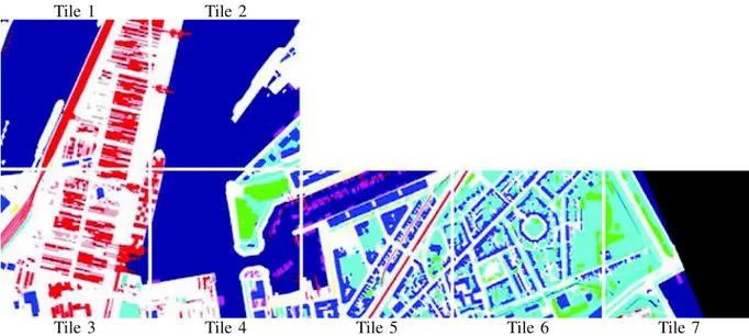
Fig. 10. Seven tiles of the ground truth built for the Data Fusion Contest 2015. To obtain the full resolution ground truth, please download the dataset on http://www.grss-ieee.org/community/technical-committees/data-fusion/2015-ieee-grss-data-fusion-contest/
Fig. 11. (left) Zooms on the ground truth (defined in Table I) superimposed to the orthoimage: It shows a good covering and matching borders. Best viewed in color. (right) Zooms to compare the original DSM and the precise DSM (d+) with respect to the RGB data. The precise DSM shows trees and cars that do not appear in the DSM provided with the Data Fusion Contest. For the sake of visibility, the DSM height range[40 m; 65 m] is mapped to the full range of image dynamics[0; 255].
carefully designed image descriptors. In the following, we refer to RGB as the three visible channels from the optical camera (see Fig. 2) and tod as the height provided in the DSM (see Fig. 3).
1) Expert Baselines: When possible, we built label-specific baselines. Most of them were single-channel filters on RGBd data. The water classifier checked if d < 45.4 m. The building classifier checked if d > 50.5 m. The road classifier (for impervious surfaces) searched for gray pixels below a given depth: max(R, G, B) − min(R, G, B) < 6 and d < 52 m. Assuming that most LiDAR systems for land observation have near-infrared (NIR) wavelengths, we projected the intensity from the LiDAR point cloud to create pseudo-NIR images. We then computed the normalized difference vegetation in-dex using(NIR − R)/(NIR + R) and fixed the threshold at0.6.
2) Support-Vector Machine (SVM) on Raw Data: As a simple baseline, we trained a SVM. Various inputs were consid-ered (and scaled to the [−1 : 1] range per channel for normalization): the RGB values of the optical dataset, RGBd values by adding the DSM, and RGBdI values,
where “I” stands for the pseudoinfrared derived from the LiDAR intensities. One SVM was trained for each class in a one-versus-all manner, using a radial basis function (RBF) kernel with internal parameters optimized by grid search. To keep the computational costs low, classifica-tion was performed on the averaged value of superpixels computed using an efficient graph-based segmentation al-gorithm [52] whose parameters were chosen to optimize the RGB/SVM classification accuracy (this segmentation was then kept in the following steps).
3) SVM on Complex Features: We tested two approaches for high-level feature extraction:
a) In the spatial–spectral domain: patches (16 × 16 or 32 × 32) were extracted with a half-patch step, in-dexed with HOGs implemented as in [53] and given the dominant label. We then trained several RBF-kernel SVMs in one-versus-all set-ups with optimal parameters found by grid search. At classification, we applied the classifier using a standard sliding window approach (same patch size and step) and smoothed the resulting map.
Fig. 12. Comparison of classification maps for tile #4 (first row) and #6 (second row), with respect to the ground truth ( GT): (experts/obj.) experts and object classifiers combined on a single map, (RGBdI) superpixels classified by SVM with RBF kernel, (HOG32/SVM) HOG features with RBF-SVM, (HSVDGr) features computed on superpixels and classified with linear SVM, (RGB Caffe), (RGB VGG) and ( RGBd VGG) CNN-features with linear SVM.
b) Using multisource information: superpixels were computed on the image, then described by hue– saturation–value (HSV) histograms combined with both the averaged value and the averaged gradient of the DSM. The classifier was learned by a linear SVM.
4) Object-Based Detectors: We also tested two methods for object-oriented detection:
a) Discriminatively trained model mixtures (DtMM) [54] built on discriminatively trained part models [53] to propose efficient object detectors for remote sensing. The model of an object category consists of a mixture of discriminative models trained on visu-ally homogeneous data: object samples are clustered on the basis of the visual appearance and for each cluster a linear SVM is trained on HOGs computed on these samples using a hard-mining procedure. In this benchmark, we used DtMM to detect cars. b) The second object detector was based on
self-organizing maps (SOM): At first, using training images only, SOMs were used to generate image segmentations according to color. Then, we built a correspondence table between semantic labels of the ground truth and the SOM classes, on the basis of the semantic, major mode for each SOM class. Fi-nally, test images were processed through the previ-ously learned SOM, and semantic labels were given to pixels using both the SOM output and the cor-respondence table. This was efficient when a good correspondence could be found between the seman-tic class and the color partition, which was the case for manmade, brightly colored objects like boats. 5) CNNs and SVM: In recent years, CNN have achieved the
best performances on various benchmarks (e.g., everyday-image classification [55]). It also has been experimented that the outputs of the intermediate layers of these deep networks could be efficiently used as features to be used in related tasks [56]. In this benchmark study, we use the AlexNet CNN model [57] as a reference. We compare three different implementations which are either replica-tions of AlexNet or small variants. All networks have been
trained on ImageNet [58] and we use the feature vector preceding the soft-max classification as input for a linear SVM (chosen for optimization issues and time constraints, but also for being less prone to overfitting). To ensure re-producibility, we make sure every network can be clearly identified in their respective article:
a) VGG (5 convolutional-layer network named fast
networkin [59]),
b) OverFeat (6 convolutional layers, also identified as
fast networkin [60]) and
c) Caffe (5 convolutional layers, standard AlexNet replication in [55]).
We generated features on 231 ∗ 231 patches extracted from the training images by a sliding window approach (step of 32 pixels) and trained a linear SVM with respect to the eight classes. At testing, the same sliding window was used, and the resulting label was given to the central 32 ∗ 32 square of the patch. This allowed to include con-text information while labeling only pixels where the class was the most likely. Moreover, we tested the contribution of LiDAR. We applied VGG to the DSM, and trained a linear SVM over the concatenated output of RGB and depth networks. We used either the given DSM (RGBd) or a more precise DSM (RGBd+) obtained by projecting
heights from the LiDAR point-cloud the xy plane for in-stant, unaveraged sensing (see Fig 11). Finally, we trained from scratch a complete AlexNet CNN with its softmax layer (using Caffe implementation) on RGBd+ data.
D. Results and Analysis
Fig. 12 illustrates the classification maps along with the ground truth, while Table II summarizes the performance mea-sures for each class and overall. The use of superpixels in-troduced spatial constraints that were visually rewarding on classification maps, especially in dense urban environment (see Fig. 12). Multisource information (marked with a ⋆ in Table II) was a key to success: The best approaches combined the image and the DSM. Working on images only, deep neural networks were solid candidates for building generic EO data classifiers. In Table II, they often outperformed the other baselines and
B (in bold)
obtained consistent results over all the eight labels. These re-sults suggest that, at least for the considered data, transferring learning from large everyday-image sets to generic datasets (as performed here for most of the competitors) is possible and more efficient than commonly used approaches. However, com-pletely retraining a CNN was even better, as shown in last row of Table II: the end-to-end trained CNN obtained the best F1-measure for 6 out of 8 classes, and an overall correct classifica-tion rate of83.32%. Finally, old recipes were still competitive on specific challenges (see Table II): NIR information proved to be crucial for classifying vegetation, while depth and col-orimetry were meaningful for buildings and water, respectively. Moreover, object-oriented methods (i.e., those that incorporate shape structure or color a priori) performed well on small ob-jects. Since objects like cars and boats did not count for much in the overall pixel proportion (see Table I), the overall pixel-wise evaluation did not do justice to these methods: The techniques performing well on the large classes resulted in better overall scores. Nevertheless, methods focusing on objects were highly effective on these classes and may have a high interest in some critical detection applications.
Summarizing, several contributions were made possible by the additional ground truth for semantic labeling we built. We tested various state-of-the-art approaches for urban classifica-tion. The main outcomes were that: 1) multisource combination is highly relevant for some specific urban classes; 2) as a generic all-purpose classifier, deep convolutional networks obtained sig-nificantly good performances; 3) transfer of learning on how to extract features from large generic-purpose image sets was a simple and highly effective approach to build EO data classi-fiers; and 4) despite this last point, training specific networks to the data being considered still payed off and led to the best results.
VI. DISCUSSION OF THE2-D CONTEST: THEWINNERS
The two winning teams awarded considered two complemen-tary aspects of the extremely high-resolution data challenge: un-derstanding data complementarity in pure statistical terms, and benchmarking what can be done with the most recent image analysis and data fusion techniques.
1) The winning team (see Section IV) used cutting edge methodology, used sparse training of CNNs to analyze what was complementary and necessary in the data pro-vided. Importantly, the networks were trained in an unsu-pervised way, so feature relations emerged from the data, without being guided by a particular set of application-specific thematic classes. They showed the structure of the data manifold and how it was organized in terms of color, texture, and LiDAR features, such as height. Fol-lowing recent computer vision momentum [61], [62], they provided understanding on data properties by analyzing the structure and information content of the convolutional filters of the network. The data proved their statistical complementarity and confirmed the need for a data fusion strategy.
2) The runner-up team (see Section V) provided a substantial effort in implementing many recent and successful tech-nologies, some well known in remote sensing (SVM) and others coming from computer vision (DPM and CNNs). These methods are starting to be considered in the remote sensing community, and the demonstration of their efficiency for this new and challenging type of data was a welcomed result, obtained by a thorough experimental design (including a fair tile training/test splitting), ground truthing, and model optimization. The results proved the efficiency of new strategies based on convolutional networks (even when simply using pretrained networks,
as in [63]–[65]) and call for new developments towards the establishment of remote-sensing-specific CNN architectures [66]. This effort also established a relevant experimental benchmark for the supervised classifica-tion of extremely high-resoluclassifica-tion data. Following this benchmark, the ground truth has been made available (http://www.grss-ieee.org/community/technical-com mittees/data-fusion/2015-ieee-grss-data-fusion-contest/). Possible future extensions of this benchmarking effort may involve further multisensor or multiresolution classifiers as well as decision-level fusion techniques.
VII. CONCLUSION OFPARTA
In this paper, we present the Data Fusion Contest 2015 orga-nized by the Image Analysis and Data Fusion Technical Com-mittee of the IEEE GRSS. In Part A, we presented the dataset and then discussed the scientific results of the winners of the 2-D contest. We invite the reader to continue to the Part B of the paper [1] for the discussion of the scientific outcome of the 3-D contest and a global discussion of the 2015 competition.
ACKNOWLEDGEMENTS
The authors wish to express their greatest appreciation to the Department of CISS, Belgian RMA, for acquiring and providing the data used in the competition and for indispensable contri-bution to the organization of the Contest, and the IEEE GRSS for continuously supporting the Annual Data Fusion Contest through funding and resources.
REFERENCES
[1] A.-V. Vo et al., “Processing of extremely high resolution LiDAR and RGB data: Outcome of the 2015 IEEE GRSS data fusion contest—Part B: 3D contest,” IEEE J. Sel. Topics Appl. Earth Observ. Remote Sens., to be published.
[2] J. Richards, Remote Sensing Digital Image Analysis. New York, NY, USA: Springer, 2013.
[3] L. Wald, “Some terms of reference in data fusion,” IEEE Trans. Geosci. Remote Sens., vol. 37, no. 3, pp. 1190–1193, May 1999.
[4] C. Pohl and J. Van Genderen, “Remote sensing image fusion: An update in the context of digital earth,” Int. J. Digit. Earth, vol. 7, no. 2, pp. 158–172, 2014.
[5] L. G´omez-Ch´ova, D. Tuia, G. Moser, and G. Camps-Valls, “Multimodal classification of remote sensing images: A review and future directions,” Proc. IEEE, vol. 103, no. 9, pp. 1560–1584, 2015.
[6] B. Waske and J. Benediktsson, “Fusion of support vector machines for classification of multisensor data,” IEEE Trans. Geosci. Remote Sens., vol. 45, no. 12, pp. 3858–3866, Dec. 2007.
[7] W. Liao et al., “Processing of thermal hyperspectral and digital color cameras: Outcome of the 2014 data fusion contest,” IEEE J. Sel. Topics Appl. Earth Observ. Remote Sens., vol. 8, no. 6, pp. 2984–2996, Jun. 2015. [8] A. Salentinig and P. Gamba, “Combining SAR-based and multispectral-based extractions to map urban areas at multiple spatial resolutions,” IEEE Geosci. Remote Sens. Mag., vol. 3, no. 3, pp. 100–112, Sep. 2016. [9] N. Longbotham et al., “Multi-modal change detection, application to the
detection of flooded areas: Outcome of the 2009–2010 data fusion contest,” IEEE J. Sel. Topics Appl. Earth Observ. Remote Sens., vol. 5, no. 1, pp. 331–342, Feb. 2012.
[10] J. Amor´os-L´opez et al., “Multitemporal fusion of Landsat/TM and EN-VISAT/MERIS for crop monitoring,” Int. J. Appl. Earth Observ. Geoin-form., vol. 23, no. 0, pp. 132–141, Aug. 2013.
[11] F. Bovolo and L. Bruzzone, “The time variable in data fusion: A change detection perspective,” IEEE Geosci. Remote Sens. Mag., vol. 3, no. 3, pp. 8–27, Sep. 2016.
[12] L. Alparone, L. Wald, J. Chanussot, C. Thomas, P. Gamba, and L. M. Bruce, “Comparison of pansharpening algorithms: Outcome of the 2006
GRS-S data fusion contest,” IEEE Trans. Geosci. Remote Sensing, vol. 45, no. 10, pp. 3012–3021, Oct. 2007.
[13] F. Gao, J. Masek, M. Schwaller, and F. Hall, “On the blending of the Landsat and MODIS surface reflectance: Predicting daily Landsat surface reflectance,” IEEE Trans. Geosci. Remote Sens., vol. 44, no. 8, pp. 2207– 2218, Aug. 2006.
[14] L. Loncan et al., “Hyperspectral pansharpening: A review,” IEEE Geosci. Remote Sens. Mag, vol. 3, no. 3, pp. 27–47, Sep. 2016.
[15] F. Pacifici, F. D. Frate, W. J. Emery, P. Gamba, and J. Chanussot, “Urban mapping using coarse sar and optical data: Outcome of the 2007 GRS-S data fusion contest,” IEEE Geosci. Remote Sens. Lett., vol. 5, no. 3, pp. 331–335, Jul. 2008.
[16] G. Licciardi et al., “Decision fusion for the classification of hyperspectral data: Outcome of the 2008 GRS-S data fusion contest,” IEEE Trans. Geosci. Remote Sens., vol. 47, no. 11, pp. 3857–3865, Nov. 2009. [17] C. Berger et al., “Multi-modal and multi-temporal data fusion: Outcome
of the 2012 GRSS Data Fusion Contest,” IEEE J. Sel. Topics Appl. Earth Observ. Remote Sens., vol. 6, no. 3, pp. 1324–1340, Jun. 2013.
[18] C. Debes et al., “Hyperspectral and LiDAR data fusion: Outcome of the 2013 GRSS data fusion contest,” IEEE J. Sel. Topics Appl. Earth Observ. Remote Sens., vol. 7, no. 6, pp. 2405–2418, Jun. 2014.
[19] M. Campos-Taberner, A. Romero, C. Gatta, and G. Camps-Valls, “Shared feature representations of LiDAR and optical images: Trading sparsity for semantic discrimination,” in Proc. IEEE Int. Geosci. Remote Sens. Symp., Milan, Italy, 2015, pp. 4169–4172.
[20] A. Lagrange et al., “Benchmarking classification of earth-observation data: From learning explicit features to convolutional networks,” in Proc. IEEE Int. Geosci. Remote Sens. Symp., Milan, Italy, 2015, pp. 4173–4176. [21] M. Cramer, D. Stallmann, and N. Haala, “Direct georeferencing using GPS/inertial exterior orientations for photogrammetric applications,” Int. Arch. Photogramm. Remote Sens., vol. 33, no. B3, pp. 198–205, 2000. [22] A. Romero, P. Radeva, and C. Gatta, “Meta-parameter free unsupervised
sparse feature learning,” IEEE Trans. Pattern Anal. Mach. Intell., vol. 37, no. 8, pp. 1716–1722, Aug. 2015.
[23] B. Koetz et al., “Fusion of imaging spectrometer and LiDAR data over combined radiative transfer models for forest canopy characterization,” Remote Sens. Environ., vol. 106, no. 4, pp. 449–459, 2007.
[24] A. F. Elaksher, “Fusion of hyperspectral images and LiDAR-based DEMs for coastal mapping,” Opt. Lasers Eng., vol. 46, no. 7, pp. 493–498, 2008.
[25] A. Swatantran, R. Dubayah, D. Roberts, M. Hofton, and J. B. Blair, “Map-ping biomass and stress in the sierra nevada using LIDAR and hyperspec-tral data fusion,” Remote Sens. Environ., vol. 115, no. 11, pp. 2917–2930, 2011.
[26] L. Naidoo, M. Cho, R. Mathieu, and G. Asner, “Classification of sa-vanna tree species, in the Greater Kruger National Park region, by in-tegrating hyperspectral and LiDAR data in a random forest data mining environment,” ISPRS J. Photogramm. Remote Sens., vol. 69, no. 0, pp. 167–179, 2012.
[27] M. Pedergnana, P. Marpu, M. Dalla Mura, J. Benediktsson, and L. Bruzzone, “Classification of remote sensing optical and LiDAR data using extended attribute profiles,” IEEE J. Sel. Topics Signal Process., vol. 6, no. 7, pp. 856–865, Nov. 2012.
[28] D. Tuia, N. Courty, and R. Flamary, “Multiclass feature learning for hy-perspectral image classification: Sparse and hierarchical solutions,” ISPRS J. Photogramm. Remote Sens., vol. 105, pp. 272–285, 2015.
[29] G. Camps-Valls, D. Tuia, L. G´omez-Chova, S. Jim´enez, and J. Malo, Eds., Remote Sensing Image Processing. LaPorte, CO, USA: Morgan & Claypool Publishers, Sep. 2011.
[30] G. Camps-Valls, D. Tuia, L. Bruzzone, and J. Atli Benediktsson, “Ad-vances in hyperspectral image classification: Earth monitoring with sta-tistical learning methods,” IEEE Signal Process. Mag., vol. 31, no. 1, pp. 45–54, Jan. 2014.
[31] R. Willett, M. Duarte, M. Davenport, and R. Baraniuk, “Sparsity and structure in hyperspectral imaging: Sensing, reconstruction, and target detection,” IEEE Signal Process. Mag., vol. 31, no. 1, pp. 116–126, Jan. 2014.
[32] Z. Wang, N. Nasrabadi, and T. Huang, “Spatial-spectral classification of hyperspectral images using discriminative dictionary designed by learning vector quantization,” IEEE Trans. Geosci. Remote Sens., vol. 52, no. 8, pp. 4808–4822, Aug. 2014.
[33] S. Yang, H. Jin, M. Wang, Y. Ren, and L. Jiao, “Data-driven compressive sampling and learning sparse coding for hyperspectral image classifi-cation,” IEEE Geosci. Remote Sens. Lett., vol. 11, no. 2, pp. 479–483, Feb. 2014.
[34] H. Sun, X. Sun, H. Wang, Y. Li, and X. Li, “Automatic target detection in high-resolution remote sensing images using spatial sparse coding bag-of-words model,” IEEE Geosci. Remote Sens. Lett., vol. 9, no. 1, pp. 109–113, Jan. 2012.
[35] A. Cheriyadat, “Unsupervised feature learning for aerial scene classifica-tion,” IEEE Trans. Geosci. Remote Sens., vol. 52, no. 1, pp. 439–451, Jan. 2014.
[36] A. Krizhevsky, I. Sutskever, and G. E. Hinton, “ImageNet classification with deep convolutional neural networks,” in Proc. Adv. Neural Inform. Process. Syst., 2012, pp. 1097–1105.
[37] K. Simonyan and A. Zisserman, “Very deep convolutional networks for large-scale image recognition,” in Proc. Int. Conf. Learn. Representations, 2015, pp. 1–14.
[38] G. E. Hinton, S. Osindero, and Y.-W. Teh, “A fast learning algorithm for deep belief nets,” Neural Comput., vol. 18, no. 7, pp. 1527–1554, Jul. 2006.
[39] Y. Bengio, P. Lamblin, D. Popovici, and H. Larochelle, “Greedy layer-wise training of deep networks,” in Proc. Adv. Neural Inform. Process. Syst., 2006, pp. 153–160.
[40] A. Coates and A. Ng, “The importance of encoding versus training with sparse coding and vector quantization,” in Proc. Int. Conf. Mach. Learn., 2011, pp. 921–928.
[41] T. Schaul, S. Zhang, and Y. LeCun, “No more pesky learning rates,” presented at Int. Conf. Machine Learning, Atlanta, GA, USA, 2013.
[42] A. Romero, C. Gatta, and G. Camps-Valls, “Unsupervised deep feature extraction for remote sensing image classification,” IEEE Trans. Geosci. Remote Sens., vol: 54, no. 3, pp. 1349–1362, 2016.
[43] D. Davies and D. Bouldin, “A cluster separation measure,” IEEE Trans. Pattern Anal. Mach. Intell., no. 2, pp. 224–227, Apr. 1979.
[44] J. Dunn, “Well-separated clusters and optimal fuzzy partitions,” J. Cybern., vol. 4, no. 1, pp. 95–104, 1974.
[45] R. B. Calinski and J. Harabasz, “A dendrite method for cluster analysis,” Commun. Statist., vol. 3, pp. 1–27, 1974.
[46] J. Leitloff, S. Hinz, and U. Stilla, “Vehicle detection in very high resolution satellite images of city areas,” IEEE Trans. Geosci. Remote Sens., vol. 48, no. 7, pp. 2795–2806, Jul. 2011.
[47] H. Randrianarivo, B. Le Saux, and M. Ferecatu, “Man-made structure de-tection with deformable part-based models,” in Proc. Int. Geosci. Remote Sens. Symp., 2013, pp. 200–203.
[48] M. Fauvel, J. Chanussot, and J. Benediktsson, “Decision fusion for the classification of urban remote sensing images,” IEEE Trans. Geosci. Re-mote Sens., vol. 44, no. 10, pp. 2828–2838, Oct. 2006.
[49] D. Tuia, F. Pacifici, M. Kanevski, and W. Emery, “Classification of very high spatial resolution imagery using mathematical morphology and sup-port vector machines,” IEEE Trans. Geosci. Remote Sens., vol. 47, no. 11, pp. 3866–3879, Nov. 2009.
[50] V. Mnih and G. Hinton, “Learning to detect roads in high-resolution aerial images,” in Proc. Eur. Conf. Comp. Vis., 2010, pp. 210–223.
[51] A. Romero, C. Gatta, and G. Camps-Valls, “Unsupervised deep feature extraction of hyperspectral images,” in Proc. WHISPERS, 2014.
[52] P. Felzenszwalb and D. Huttenlocher, “Efficient graph-based image seg-mentation,” Int. J. Comp. Vis., vol. 59, no. 2, pp. 167–181, 2004. [53] P. Felzenszwalb, R. Girshick, D. McAllester, and D. Ramanan,
“Ob-ject detection with discriminatively trained part-based models,” IEEE Trans. Pattern Anal. Mach. Intell., vol. 32, no. 9, pp. 1627–1645, Sep. 2010.
[54] H. Randrianarivo, B. Le Saux, M. Crucianu, and M. Ferecatu, “Discriminatively-trained model mixture for object detection in aerial im-ages,” presented at the Image Information Mining, Bucharest, Romania, 2015.
[55] Y. Jia et al., “Caffe: Convolutional architecture for fast feature embedding,” in Proc. 22nd ACM Int. Co. Multimedia, pp. 675–678, 2014.
[56] J. Yosinski, J. Clune, G. Hinton, and H. Lipson, “How transferable are features in deep neural networks?” in Proc. Adv. Neural Inform. Process. Syst., 2014, pp. 3320–3328.
[57] A. Krizhevsky, I. Sutskever, and G. Hinton, “ImageNet classification with deep convolutional neural networks,” in Proc. Adv. Neural Inform. Pro-cess. Syst., 2012, pp. 1097–1105.
[58] J. Deng, W. Dong, R. Socher, L.-J. Li, K. Li, and L. Fei-Fei, “ImageNet: A large-scale hierarchical image database,” in Proc. Comput. Vis. Pattern Recog., 2009, pp. 248–255.
[59] K. Chatfield, K. Simonyan, A. Vedaldi, and A. Zisserman, “Return of the devil in the details: Delving deep into convolutional nets,” in Proc. Brit. Mach. Vis. Conf., 2014.
[60] P. Sermanet, D. Eigen, X. Zhang, M. Mathieu, R. Fergus, and Y. LeCun, “Overfeat: Integrated recognition, localization and detection using convo-lutional networks,” in Proc. Int. Conf. Learn. Rep., 2014. [Online]. Avail-able: http://openreview.net/document/d332e77d-459a-4af8-b3ed-55ba [61] A. Mahendran and A. Vedaldi, “Understanding deep image representations
by inverting them,” presented at the Computer Vision Pattern Recognition, Boston, MA, USA, 2015.
[62] K. Lenc and A. Vedaldi, “Understanding image representations by mea-suring their equivariance and equivalence,” presented at the Computer Vision Pattern Recognition, Boston, MA, USA, 2015.
[63] S. Workman and N. Jacobs, “On the location dependence of convolutional neural network features,” in Proc. Computer Vision Pattern Recognition Worshops: EarthVision, Jun. 2015, pp. 70–78.
[64] O. A. B. Penatti, K. Nogueira, and J. A. dos Santos, “Do deep features generalize from everyday objects to remote sensing and aerial scenes domains?” in Proc. Comput. Vis. Pattern Recog. Worshops: EarthVision, Jun. 2015, pp. 44–51.
[65] D. Marmanis, M. Datcu, T. Esch, and U. Stilla, “Deep-learning earth observation classification using ImageNet pre-trained networks,” IEEE Geosci. Remote Sens. Lett., vol. 13, no. 1, pp. 105–109, Jan. 2016.
[66] S. Paisitkriangkrai, J. Sherrah, P. Janney, and A. Van-Den Hengel, “Effec-tive semantic pixel labelling with convolutional networks and conditional random fields,” in Proc. Comput. Vis. Pattern Recog. Worshops: EarthVi-sion, Jun. 2015, pp. 36–43.