an author's
https://oatao.univ-toulouse.fr/26911
https://doi.org/10.1017/aer.2019.126
Blazquez, Emmanuel and Beauregard, Laurent and Lizy-Destrez, Stéphanie and Ankersen, Finn and Capolupo,
Francesco Rendezvous design in a cislunar near rectilinear Halo orbit. (2020) Aeronautical Journal, 124 (1276).
821-837. ISSN 0001-9240
Optimal rendezvous trajectory between Sample Return Orbiter and Orbiting
Sample Container in a Mars Sample Return mission
Alberto Fossà
a,b,∗, Carlo Bettanini
b,caISAE Supaéro - Institut Supérieur de l’Aéronautique et de l'Espace, 10 Avenue Édouard Belin, Toulouse, France bDepartment of Industrial Engineering, University of Padova, Via Venezia 1, Padova, Italy
cCISAS -Center for Studies and Activities for Space“G.Colombo”, University of Padova, Via Venezia 15, Padova, Italy
Keywords:
Two-impulse rendezvous Minimum energy
Non-coplanar elliptical orbits Orbit transfer
Sample return
A B S T R A C T
A trajectory optimization problem is examined to determine the most fuel-efficient rendezvous trajectory be-tween spacecrafts in different orbits. To explore the whole range of feasible solutions, the wait time and the total time offlight are treated as free parameters while the initial and transfer orbits are not restricted to a particular one. To improve the accuracy of the numerical computation, the Kepler's time offlight equation is posed in terms of universal variables while the Lagrange coefficients are employed to obtain three-dimensional orbit in-formation. The optimal rendezvous trajectory is then obtained enforcing the determined necessary conditions to be satisfied given only the initial state vectors of the involved spacecrafts. Two optimal rendezvous trajectories between a Sample Return Orbiter (SRO) and an Orbiting Sample Container (OS) are computed in the context of a future Mars Sample Return mission to demonstrate the reliability of the proposed solution. Finally, orbital perturbations due to the real shape of planet Mars and the solar radiation pressure are taken into account to determine the additional energy required to compensate these perturbations while performing the rendezvous manoeuvre.
1. Introduction 1.1. Context
Mars exploration is a milestone in the Global Exploration Roadmap proposed by the International Space Exploration Coordination Group [1] as is a common interest in the future exploration activity by several international agencies. It provides global opportunities for scientific study and technological advancement and features at first robotic missions with the long-term goal of crewed landers on Mars [2] as a logical step for expanding human presence in the solar system. To en-able sustainen-able human missions, a better understanding of environ-mental conditions and potential in-situ material utilization [3] shall be conducted by analysing samples from planetary surface.
Consequently, a Mars Sample Return mission [4–6] is perceived as a powerful way to answer most of the open questions about the red planet, enabling the international network of scientific laboratories and research facilities to conduct detailed analysis directly on the collected samples. The latest proposals for such a mission [5,7] subdivide the complex task into four different phases: samples collection from the surface of Mars and sealing in an Orbiting Sample Container (OS),
launch of the OS in a parking orbit around the red planet, capture of the OS by a Sample Return Orbiter (SRO) and return of the SRO towards the Earth.
Due to multiple constraints on the SRO manoeuvring capabilities [8], the most fuel-efficient transfer trajectory to capture the passive OS has to be determined in order to increase the reliability of the whole mission. Assuming thefirst phase to be accomplished by the upcoming Mars 2020 rover, the OS will be placed in a low-inclined circular orbit while the SRO operating orbit will be most likely sun-synchronous for scientific purposes [4]. As a consequence, the most fuel-efficient transfer between two non-coplanar elliptical orbits has to be de-termined to satisfy the mission requirements.
1.2. Optimal control problem
The optimal control problem is then formulated assuming that the SRO will execute two impulsive manoeuvres to leave the initial parking orbit and perform thefinal rendezvous with the OS. Then, a specific approach is proposed to compute the optimal rendezvous trajectory between an active chaser and a passive target assuming that only the respective initial state vectors are known [9,10]. To explore the whole
https://doi.org/10.1016/j.actaastro.2020.02.046
∗Corresponding author. ISAE Supaéro - Institut Supérieur de l’Aéronautique et de l’Espace, 10 Avenue Édouard Belin, Toulouse, France.
range of feasible solutions, the wait time spent by the chaser in its in-itial orbit and the total time offlight required to complete the man-oeuvre are left as free parameters to be determined. Finally, is to be noticed that the proposed approach is substantially different from most of the work presented in the literature, since the last relies frequently on the well known solution to thefixed-time Lambert problem.
In this work two meaningful rendezvous conditions are derived and it will be proven that the control energy required to perform the ren-dezvous is a minimum only if they are both satisfied [10]. These con-ditions are then adjoined with the required equations of motion to obtain a unique set of equations to be solved for the optimal transfer trajectory providing only the chaser and target's initial state vectors.
The proposed implementation is firstly validated on a test case proposed by Shirazi et al. [11] and then employed in the context of a future Mars Sample Return mission. For the last case, two optimal rendezvous trajectories that allow the SRO to capture the OS will be computed taking advantage of the developed optimization framework. For both cases, the numerical results and the required velocity changes are compared to the fixed-time solution to the Lambert problem to demonstrate the effectiveness of the proposed approach while searching for the most fuel-efficient transfer.
Since the whole optimization framework relies on the restricted two-body problem approximation, the last chapter relaxes this as-sumption to estimate the additional velocity changes to be undertaken by the SRO when the effects of the Mars static gravitational field and the solar radiation pressure are taken into account. A parametric study is conducted here to determine the impact in the overallΔv due to variations in each orbital parameter of both SRO and OS.
The paper is organized as follows. Before being applied in the subsequent work, the Kepler's equation in terms of universal variables and the Lagrange coefficients are briefly revised in chapter 2. Secondly, chapter 3 defines a cost index to evaluate the optimal solution and resumes the derivation of the two rendezvous conditions. The chapter concludes with the presentation of the whole set of equations to be solved for the optimal rendezvous trajectory. Thirdly, chapter 4 com-pares the test case results with the ones presented in the literature while in chapter 5 two possible solutions for the Mars Sample Return mission are computed and validated comparing the proposed approach with the solution to the Lambert problem. Finally, chapter 6 presents the con-sequences of the considered orbital perturbations on the SRO perfor-mances while chapter 7 draws some general conclusions on the con-ducted work.
2. Mathematical background 2.1. Kepler's equation
To simplify the spacecrafts' equations of motion and the derivation of the optimality conditions the first fundamental assumption is to consider the planet Mars to be a spherical and homogeneous body. Moreover, the gravitational forces due to other celestial bodies in the solar system and non-gravitational phenomena such as the solar ra-diation pressure are neglected. Under these hypothesis the subsequent work is formulated in the restricted two-body problem framework, for which the well-known Kepler's equation holds [12]:
= −
Me E esinE (1)
WithMe mean motion, E eccentric anomaly and e eccentricity of the
orbit. HereMe= μ a/ 3(t−tp)where t is the time at which the position is computed while tpis referred to the periapsis passage.
However, equation(1)is valid only for elliptical orbits withe<1
and its numerical solution for t when the spacecraft's position is known becomes inaccurate for almost parabolic orbits with e→1. To over-come this issue an alternative formulation based on the universal variables is introduced in section2.2.
2.2. Universal variables
Starting from the classical orbital elements, the universal variable is defined as [13]: = x μ r ˙ (2) whereμ is the gravitational parameter of the central body and r the spacecraft's position.
Then, assumingt0=0forx=0 and denoting with[ ,r v0 0]the state
vector of the spacecraft at t0the two quantities r t, can be expressed as
functions of x as given by equations(3) and (4): = ⎛ ⎝ − ⎞ ⎠ + ⎛ ⎝ − ⎞ ⎠ + r v μ t a x a x a a μ x a r a x a sin 1 cos sin T 0 0 0 (3) = + ⎡ ⎣ ⎢ + ⎛⎝ − ⎞⎠ ⎤ ⎦ ⎥ r v r a a μa x a r a x a sin 1 cos T 0 0 0 (4) 2.3. Lagrange coefficients
Finally, since in the restricted two-body problem the spacecraft's motion is confined within a plane its state vector[ , ]r v at time t can be expressed as a linear combination of[ ,r v0 0]at time t0as follows [12]:
= +
r fr0 gv0 (5)
= +
v f˙r0 g˙v0 (6)
Where f g f g, , ˙ , ˙ are the four Lagrange coefficients whose expressions for an elliptical orbit are given by equations(7)–(10)[13]:
= − ⎛ ⎝ − ⎞ ⎠ f a r x a 1 1 cos 0 (7) = − ⎛ ⎝ − ⎞ ⎠ g t a μ x a x a sin (8) = − f μa rr x a ˙ sin 0 (9) = − ⎛ ⎝ − ⎞ ⎠ g a r x a ˙ 1 1 cos (10) Consequently, the three-dimensional motion of the spacecraft in a given orbit can be fully determined computing its state vector[ , ]r v at any time t from the knowledge of [ ,r v0 0] at t0 solving equations
(3)–(10). This formulation is used in chapter 3 to derive the necessary conditions for an optimal rendezvous manoeuvre and in chapters 4–5 to obtain a numerical solution in the proposed scenarios.
3. Optimal control problem 3.1. Performance index
To solve for the most energy-efficient rendezvous trajectory a cost or performance indexJ is defined and the necessary conditions for its
minimum derived analytically before proceeding with a numerical computation of the optimal solution.
Since the chaser performs the rendezvous manoeuvre with two consecutive impulsive burns, minimize the control energy is equivalent to minimize the instantaneous changes in the spacecraft's specific ki-netic energy [14] and thus a convenient expression forJis given by:
= 1 v v + v v 2Δ Δ 1 2Δ Δ T T 1 1 2 2 J (11)
initial orbit to the transfer trajectory while vΔ 2is applied after t to leave
the transfer trajectory and enter the target orbit. 3.2. Constraints
Afirst constraint has to be added to the problem such that at each time the two spacecrafts follows a Keplerian orbit satisfying equations (3) and (4). This condition is easily expressed by equation(12)where
= ∈
η [ ,η η,η]T
1 2 3 R3and the three components are given by equations
(13)–(15). = η(‾, , , , , Δ )x x x t t1 1 v1 0 (12) = ⎛ ⎝ − ⎞ ⎠ + ⎛ ⎝ − ⎞ ⎠ + − r v η x t a x a x a a μ x a r a x a μ t ( ¯, ) ¯ ¯ ¯ sin ¯ ¯ ¯¯ ¯ 1 cos ¯ ¯ ¯ ¯ sin ¯ ¯ T 1 0 0 0 (13) ⎜ ⎟ ⎜ ⎟ = ⎛ ⎝ − ⎞ ⎠ + ⎛ ⎝ − ⎞ ⎠ + − r v η x t a x a x a a μ x a r a x a μ t ( , ) sin 1 cos sin T 2 1 1 0 1 0 1 0 0 0 0 1 0 0 0 1 0 1 (14) ⎜ ⎟ ⎜ ⎟ = ⎛ ⎝ − ⎞ ⎠ + + ⎛ ⎝ − ⎞ ⎠ + − − v r v v η x x t t a x a x a a μ x a r a x a μ t t ( , , , , Δ ) sin ( Δ ) 1 cos sin ( ) T 3 1 1 1 1 1 1 1 1 1 1 1 1 1 1 1 (15) Here 13 describes the motion of the target in an orbit with semi-major axisa‾, while 14 and 15 represent the motion of the chaser in its initial
orbit and in a transfer trajectory characterized bya0anda1respectively.
Moreover, equation(13)holds in the time interval[ , ]t0 t, 14 in t[ , ]0 t1
and 15 in[ , ]t t1 where t1is the wait time and t the total time offlight.
Secondly, two more constraints are enforced to guarantee that at time t the two spacecrafts move along the same orbit and have the same positions as required by equations(16) and (17):
− =
r r
‾ 0 (16)
− + =
v‾ (v Δ )v2 0 (17)
Finally, the state vector[ ,r v1 1]of the chaser at t1and the two state
vectors[ , ]r v and r v[‾, ‾] for both spacecrafts at the final time t can be evaluated from equations(5) and (6):
= + r1( , )x t1 1 f0 0r g0 0v (18) = + v1( )x1 f˙0 0r g˙0 0v (19) = + + r( , , , , Δ )x x t t1 1 v1 f1 1r g1(v1 Δ )v1 (20) = + + v( , , Δ )x x1 v1 f1 1˙r g˙ (1 v1 Δ )v1 (21) = + r x t fr gv ‾ (‾, ) ‾ ‾0 ‾ ‾0 (22) = + v‾ (‾)x f‾˙ ‾r0 g‾˙ ‾v0 (23)
While the semi-major axis of the transfer trajectorya1and thefinal
orbit radius r can be computed from the energy equation and expression 4: + + − = − v v v v μ r μ a ( Δ ) ( Δ ) 2 2 T 1 1 1 1 1 1 (24) ⎜ ⎟ = + ⎡ ⎣ ⎢ + + ⎛ ⎝ − ⎞ ⎠ ⎤ ⎦ ⎥ r v v r a a μa x a r a x a ( Δ ) sin 1 cos T 1 1 1 1 1 1 1 1 1 1 (25) 3.3. Problem statement
Considering the performance indexJ defined in 11 and the con-straints 12, 16 and 17, the optimal control problem is stated as follows: given[ ,r v0 0]and r v[‾ , ‾ ]0 0 at time t0determine the wait time t1, the total
time offlight t and the velocity changes vΔ , Δ1 v2minimizingJsubject
to: ⎧ ⎨ ⎩ = − = − + = η v r r v v v x x x t t (‾, , , , , Δ ) 0 ‾ 0 ‾ ( Δ ) 0 1 1 1 2 (26) 3.4. Necessary conditions
Starting from the definition ofJgiven by equation(11)and taking into account equation (26), a well-defined constrained optimization problem is obtained with 11 scalar unknowns[‾, , , , , Δ , Δ ]x x x t t1 1 v1 v2
and 9 constraints. The problem can be converted in an unconstrained optimization problem defining the augmented performance indexH, also known as the Hamiltonian, with the introduction of the Lagrange multipliersλ ϕ ψ, , ∈R3[10]: = + + − + − + v v λ η v ϕ r r ψ v v v x x x t t (Δ , Δ ) (‾, , , , , Δ ) (‾ ) (‾ ( Δ )) T T T 1 2 1 1 1 2 H J (27) The necessary conditions to minimizeH with respect to the aug-mented variables are given by equations(28)–(34):
∂ ∂ = ∂ ∂ + ∂ ∂ + ∂ ∂ = ϕ r ψ v x λ η x x x ‾ ‾ ‾ ‾ ‾ ‾ 0 T T 1 1 H (28) ∂ ∂ = ∂ ∂ + ∂ ∂ − ∂ ∂ − ∂ ∂ = ϕ r ψ v x λ η x λ η x x x 0 T T 1 2 2 1 3 3 1 1 1 H (29) ∂ ∂ = ∂ ∂ − ∂ ∂ − ∂ ∂ = ϕ r ψ v x λ η x x x 0 T T 3 3 H (30) ∂ ∂ = − + + ⎛⎝ ∂ ∂ − ∂ ∂ ⎞⎠= ϕ r r t μ λ( λ) t t ‾ 0 T 1 3 H (31) ∂ ∂ = − + ∂ ∂ − ∂ ∂ − ∂ ∂ = ϕ r ψ v t μ λ λ η t t t 0 T T 1 2 3 3 1 1 1 H (32) ∂ ∂ = ∂ ∂ + ∂ ∂ − ∂ ∂ − ∂ ∂ = v v v ϕ r v ψ v v λ η Δ Δ Δ Δ Δ 0 T T 1 1 3 3 1 1 1 H J (33) ∂ ∂ = ∂ ∂ − × = v v ψ I Δ Δ 0 T 2 2 3 3 H J (34) Those expressions can be manipulated and combined together to obtain two meaningful scalar equationsh h1, 2 denoted as rendezvous
conditions and equivalent to equations(28)–(34)[10]:
= − ⎡ ⎣ ⎢ − + − ⎤ ⎦ ⎥+ − = − ∂ ∂ ∂ ∂ ∂ ∂ ∂ ∂ ∂ ∂ ∂ ∂
(
)
(
)
(
)
v v L L v h (Δ Δ ) Δ 0 r r r r v v T T x x r μ t t T x x 1 1 2 1 01 ¯ ¯ ¯ 2 ¯ ¯ (35) = − ⎡ ⎣ − + ⎤⎦ + ⎡ ⎣ − + ⎤⎦= − ∂ ∂ ∂ ∂ ∂ ∂ ∂ ∂ ∂ ∂ ∂ ∂(
)
(
)
v v L L v h l l (Δ Δ ) Δ 0 r r r v v v T T x μ r x t T x μ r x t 2 1 2 1 01 2 2 2 1 1 1 1 1 1 (36)Where L0,L1and l2are defined as follows:
= ∂ ∂ − ∂ ∂ ∂ ∂ L r v r v r x η Δ 1 Δ 0 1 3 1 (37) = ∂ ∂ − ∂ ∂ ∂ ∂ L v v v v r x η Δ 1 Δ 1 1 3 1 (38)
⎜ ⎟ = ⎛ ⎝ ∂ ∂ + ∂ ∂ ⎞ ⎠ l r μ r η x η t 1 2 1 3 1 3 1 (39)
Combining expressions 26, 35 and 36 the whole set of equations that satisfies the optimality conditions, the equations of motion and the constraints on thefinal state vectors is obtained as:
⎧ ⎨ ⎪ ⎪ ⎩ ⎪ ⎪ = − = − + = = = η v r r v v v v v v v x x x t t h x x t t h x x t t (‾, , , , , Δ ) 0 ‾ 0 ‾ ( Δ ) 0 (‾, , , , Δ , Δ ) 0 ( , , , , Δ , Δ ) 0 1 1 1 2 1 1 1 2 2 1 1 1 2 (40)
Which is a non-linear system that has to be solved numerically to de-termine[‾, , , , , Δ , Δ ]x x x t t v v T ∈
1 1 1 2 R11that corresponds to a minimum
ofJ.
Then, since the parametersa r1, ,r v1, 1that appears in 40 are a priori
unknowns, the four equations(18), (19), (24) and (25)have to be ad-joined to the system and the relations 20 to 23 taken into account to derive afinal set of equations whose solution is computed from the only knowledge of[ ,r v0 0]and r v[‾ , ‾ ]0 0 at time t0.
The whole system can be conveniently expressed as:
=
X
F( ) 0 (41)
WhereX=[ ,a x x x r t t, , ‾, , , , , , Δ , Δ ]r v v v T ∈
1 1 1 1 1 1 2 R19and F is given by:
⎧ ⎨ ⎪ ⎪ ⎪ ⎪ ⎪ ⎪ ⎪ ⎩ ⎪ ⎪ ⎪ ⎪ ⎪ ⎪ ⎪ − + = + ⎡ ⎣ ⎢ + − ⎤ ⎦ ⎥− = + − = + − = = + − − + = + − − + − = = = + + +
(
)
r v r r v v η v r v r v v r v r v v v v v v v a a r f g f g x x x t t f g f g f g f g h x x t t h x x t t 0 sin 1 cos 0 0 ˙ ˙ 0 (‾, , , , , Δ ) 0 ‾ ‾ ‾ ‾ ( Δ ) 0 ‾˙ ‾ ‾˙ ‾ ˙ ˙ ( Δ ) Δ 0 (‾, , , , Δ , Δ ) 0 ( , , , , Δ , Δ ) 0 v v v v r v v μ r μ a μa x a r a x a ( Δ ) ( Δ ) 2 2 1 1 ( Δ ) 0 0 0 0 1 0 0 0 0 1 1 1 1 0 0 1 1 1 1 1 0 0 1 1 1 1 1 2 1 1 1 2 2 1 1 1 2 T T 1 1 1 1 1 1 1 1 1 1 1 1 1 1 (42) 4. Numerical exampleBefore being applied in the context of a future Mars Sample Return mission, the algorithm developed in chapter 3 is tested on a reference case proposed by Shirazi et al. [11]. Two non-coplanar, elliptical Earth orbits are selected and an optimal solution is sought for the most effi-cient rendezvous trajectory between the two spacecrafts. The chaser is initially located at the perigee of its orbit while the target initial con-ditions are chosen such that transfer time and burn locations coincide with the already published results. This adjustment is needed since the previous work considers only an optimal transfer between the two or-bits without any requirement on the phasing between two spacecrafts. The whole set of initial classical orbital elements is given inTable 1 with a semi-major axis, e eccentricity, Ω right ascension of the as-cending node, i inclination, ω argument of periapsis and θ true anomaly.
The optimal rendezvous trajectory is determined solving equation (41)knowing the state vectors r v[‾ , ‾ ]0 0 and[ ,r v0 0]computed from data in
Table 1as follows [12]: = − = = − − − = − r v r v km km s km km s ‾ [30632.3974 9551.6183 36506.2697] ‾ [0.3969 1.9478 0.4731] / [ 6657.0680 2158.1938 5722.5209] [1.5883 7.0519 0.8119] / T T T T 0 0 0 0 (43)
MATLAB® R2019a is used to implement the proposed algorithms and obtain the corresponding results. All computations are performed on a Lenovo Y50-70 running Ubuntu 18.04 LTS with an Intel® Core™ i7-4720HQ CPU @ 2.60 GHz processor and 8 GB RAM.
Local optimization techniques are adopted to numerically solve equation (41) and thus different trajectories can be generated de-pending on the provided initial guess X0. Multiple sub-optimal transfers
are obtained as solutions of the Lambert problem and the closest one to the global optima is selected as initial guess for the developed optimi-zation algorithm. If X0is in the basin of Xopt the convergence of the
iterative routines is guaranteed and a solution is found without trouble. Thefixed-time transfer admits two different solutions, one corre-sponding to a change in true anomalyΔθ<180∘ and the other with
> ∘
θ
Δ 180 , where Δθ=θ−θ1 is the difference in the chaser's true
anomaly between the two impulsive burnsΔ , Δv1 v2. Only the second
solution is considered here since it corresponds to the results already available in the literature.
Equation(41)is then solved taking14.6saverage CPU time leading to the following optimal solutionXopt:
= = = = = = = = − − − = − = − = − − r v v v a km x x x r km t s t s km km s km s km s 21751.0401 62.7782 608.8852 ‾ 382.2524 26930.8146 911.7310 24993.6024 [ 3901.5075 7678.1036 3882.8137] [4.1862 4.6727 3.1576] / Δ [0.5811 0.7221 0.6432] / Δ [ 0.2126 0.0621 0.9821] / T T T T 1 1 1 1 1 1 2 (44)
From which the corresponding performance indexJopt, totalΔv,
transfer trajectory's time offlightTOF and chaser'sfinal state vector
r v [ , ]are retrieved: = = = − = = = − − − r v v km s TOF t t s km km s 1.1433 Δ 2.1350 / 24081.8713 [4660.0549 25936.6561 5553.6371] [ 2.6126 0.9242 3.1136] / opt tot T T 1 J (45) These results are inline with the ones obtained by the previous authors thus validating the proposed algorithm and implementation.
Finally, the classical orbital elements for the rendezvous trajectory are computed from[ ,r v1 1]and[ , ]r v given by 44, 45 obtaining the
re-sults inTable 2[12].Fig. 1depicts both the optimal transfer trajectory and the two initial orbits in an inertial reference frame centered on planet Earth.
The optimal solutionXoptis then validated comparing the obtained
value Jopt with the performance indexes corresponding to multiple
solutions of the Lambert problem for different values oft t1, centered in
the optimal ones presented in 44. FromFigs. 2 and 3is possible to verify thatJopt= min[ , ]t t1 J thus validating the proposed approach.
Finally, different contour lines for bothh h1, 2are plotted inFig. 4to
demonstrate that X=Xopt only if h1=h2=0, namely if the two
Table 1
Classical orbital elements for the test case orbits.
S C/ a km( ) e( )− Ω ( )° i( )° ω( )° θ0( )°
Target 32,600 0.5 270 50 265 173.6664
Chaser 11,300 0.2 275 40 280 0
Table 2
Optimal transfer trajectory's classical orbital elements in the test case scenario.
a1(km) e( )− Ω ( )° i( )° ω( )° θ1( )° θ( )° 21751.0401 0.5737 273.9006 40.8897 304.6363 17.0650 217.0013
rendezvous conditions are both satisfied. 5. Application to Mars Sample Return mission 5.1. Initial orbits
Due to the mission complexity and costs, the initial orbits of the two spacecrafts have to be chosen such that the probability of failure are minimized and an adequate scientific return is guaranteed. As a
consequence, the landing mass of the probe that carries the OS down to the Mars surface has to be minimized to increase the chances of a successful touchdown. Since most of its weight is due to the propellant required to boost the OS back into orbit, the launch phase from the red planet has to be designed to minimize propellant consumption. On the other side, a minimum safe altitude must be achieved to ease the ren-dezvous manoeuvre performed by the SRO. For these reasons, a circular orbit at500kmaltitude with =i 18.4386∘N corresponding to a launch
due east from Jezero Crater, the selected landing site for the Mars 2020 mission [15], has been chosen as a representative trajectory for the passive target.
On the other hand, the SRO will be equipped with appropriate scientific instruments to perform in-orbit measurements during surface operations of the lander. Due to its interesting properties, a sun-syn-chronous orbit witha=4222kmande=0.1362[16] has beenfinally selected as an ideal candidate for the SRO parking orbit.
The complete set of classical orbital elements that defines the spacecrafts initial orbits is presented inTable 3.
These data are then converted in the corresponding state vectors r v
[‾ , ‾ ]0 0 and[ ,r v0 0]to be employed in the solution of equation(41):
= = = − = − r v r v km km s km km s ‾ [3897 0 0] ‾ [0 3.1449 1.0485] / [0 258.9441 3637.7956] [ 3.6528 0 0] / T T T T 0 0 0 0 (46)
As explained in section4, depending on the provided initial guess two different solutions can be computed, one corresponding to a change in true anomalyΔθ<180 and the other with∘ Δθ>180 . Both of them∘
have been considered in this study and the optimal rendezvous trajec-tories obtained from those guesses are presented in sections5.2 and 5.4. 5.2. Short path scenario
Afirst optimal solution is searched between the transfer trajectories characterized byΔθ<180 . With an average CPU time lower than∘ 3s
Fig. 1. Initial orbits and optimal transfer trajectory in the test case scenario.
Fig. 2. Performance indexJfor varying t t1, in the test case scenario.
Fig. 3. Performance indexJfor varying t t1, in the test case scenario.
Fig. 4. Rendezvous conditions h h1, 2for varying t t1, in the test case scenario.
Table 3
Classical orbital elements for the Mars Sample Return orbits.
S C/ a km( ) e( )− Ω ( )° i( )° ω( )° θ0( )°
OS 3897 0 0 18.4386 0 0
Xoptis then obtained as follows: = = = = = = = = − − = − − = − − = − r v v v a km x x x r km t s t s km km s km s km s 4080.0510 508.5480 207.0184 ‾ 776.8537 3897 10194.4513 14628.6477 [ 4181.0932 32.6174 458.2276] [ 0.0867 0.2269 3.1876] / Δ [ 0.0982 2.0671 0.6486] / Δ [0.5365 1.1153 1.6870] / T T T T 1 1 1 1 1 1 2 (47)
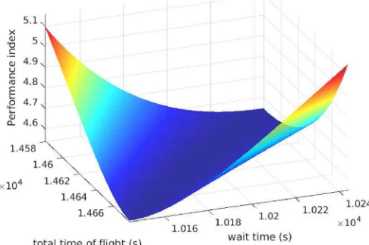
From which the corresponding performance index Jopt, transfer
trajectory's time offlightTOF and chaser'sfinal state vector[ , ]r v are retrieved: = = − = = − − = − r v TOF t t s km km s 4.5406 4434.1964 [3868.0498 449.7903 149.9619] [ 0.1332 2.0062 2.7277] / opt T T 1 J (48) Finally, the classical orbital elements for the rendezvous trajectory are given inTable 4whileFig. 5depicts both the transfer trajectory and the two initial orbits in an inertial reference frame centered at planet Mars.
5.3. Validation of proposed numerical method for short path scenario Similarly as before, the optimal solutionXoptis validated comparing
the results with multiple solutions of the Lambert problem for different values of t t1, . From Figs. 6 and 7 is possible to verify that
= min
opt [ , ]t t1
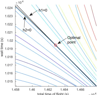
J J while Fig. 8 demonstrates that X=Xopt only if
= =
h1 h2 0, namely if the two rendezvous conditions are both satisfied.
5.4. Long path scenario
Following a similar approach, a second optimal solution is searched between the transfer trajectories withΔθ>180 . With an average CPU∘
time of5.3s, the different components ofXoptare obtained as:
= = = = = = = = − = − − = − = − r v v v a km x x x r km t s t s km km s km s km s 4043.1058 718.0996 199.8981 ‾ 986.2006 3897 14830.2442 18570.7816 [4176.0966 24.0371 337.6865] [ 0.1781 0.2275 3.1963] / Δ [0.1636 2.0769 0.6604] / Δ [0.2749 1.1442 1.6823] / T T T T 1 1 1 1 1 1 2 (49)
And the performance indexJopt, transfer trajectory's time offlightTOF
and chaser'sfinal state vector[ , ]r v are given by:
= = − = = − − − = − − r v TOF t t s km km s 4.4958 3740.5374 [ 3881.2410 332.1370 110.7358] [0.0229 1.9880 2.7266] / opt T T 1 J (50) Finally, the classical orbital elements for the rendezvous trajectory
Table 4
Optimal transfer trajectory's classical orbital elements in the short path sce-nario.
a1(km) e( )− Ω ( )° i( )° ω( )° θ1( )° θ( )° 4080.0510 0.1453 354.9746 53.9313 77.4148 110.3308 279.8565
Fig. 5. Initial orbits and optimal transfer trajectory in the short path scenario.
Fig. 6. Performance indexJfor varying t t1, in the short path scenario.
are reported inTable 5.Fig. 9depicts the different trajectories in the same reference frame as 5.
5.5. Validation of proposed numerical method for long path scenario Once again, solving the Lambert problem for different values oft t1,
demonstrates that Jopt= min[ , ]t t1 J as well as that X=Xopt only if
= =
h1 h2 0. Those results are illustrated inFigs. 10–12.
6. Effects of orbital perturbations
The extensive elaboration of data coming from the orbiting space-crafts Mars Global Surveyor (MGS), Mars Odyssey and Mars Reconnaissance Orbiter (MRO) has produced in recent years noticeable improvement in the understanding of the characteristics of the Mars
gravitationalfield [17].
Orbital evolution of spacecrafts around the planet are in fact the results of a combined effect of Mars static gravitational field, time variation of the gravitationalfield induced by mass exchange between
Fig. 8. Rendezvous conditions h h1, 2for varying t t1, in the short path scenario.
Table 5
Optimal transfer trajectory's classical orbital elements in the long path scenario.
a1(km) e( )− Ω ( )° i( )° ω( )° θ1( )° θ( )° 4043.1058 0.0756 3.7051 53.9405 116.7048 237.5733 65.3096
Fig. 9. Initial orbits and optimal transfer trajectory in the long path scenario.
Fig. 10. Performance indexJfor varying t t1, in the long path scenario.
Fig. 11. Performance indexJfor varying t t1, in the long path scenario.
the atmosphere and the ice caps (with periodicity linked to the 11 year cycle of solar activity) and time variation of the gravitationalfield in-duced by the tides. Contributions by non conservative forces as the ones by atmospheric drag and solar radiation pressure shall be taken into consideration depending on orbit type and altitude as well as third body effects due to Moons or the Sun.
When considering the baseline orbiting sample return mission in this work some contributions to Mars gravityfield perturbation may be disregarded, due to their limited variation in the time range expected for the overall intercept manoeuvre (around 5 h) and just the effect of the Mars staticfield and solar radiation pressure may produce effective variations on orbital parameters.
Due to its lumpy character, the static gravitationalfield shall be simulated with a model with high order harmonics. While low order zonal harmonics are the most important factor affecting spacecraft's drift of motion, tesseral terms provide not negligible zero mean peri-odical oscillations. Although recently developed new JPL Mars gravity fields (MRO110B and MRO110B2) show resolution near degree 90, the model used in this work has been limited to order 60 by using a Goddard Mars Gravity Model 2 (GMM2).
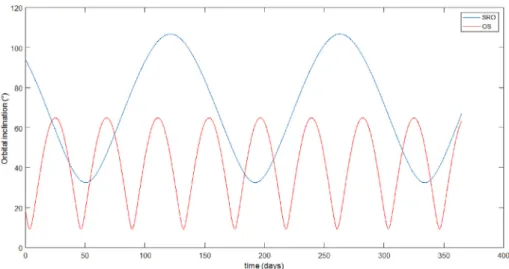
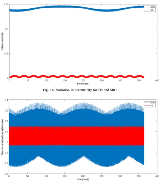
The orbits of OS and SRO have been propagated using the GMM2 field model and considering solar radiation pressure for 365 days in order to investigate the worst case in terms of deviations of orbital parameters in a 5 h time range. Such maximum variations have been then considered as a 3 sigma 99.9% confidence uncertainty value to be taken into account for each Keplerian parameter in the optimization algorithm. The results for orbit inclination, eccentricity, semi-major axis, AOP and RAAN are reported inFigs. 13–15.
As a result, the 3 sigma uncertainty values reported inTable 6have been considered for OS and SRO in a 5 and 4 h time range respectively. At this point a systematic analysis has been conducted to determine the impact of those changes in the overallΔvrequired for the rendez-vous manoeuvre. For both short and long path scenarios four different parametric studies have been performed applying those variations after the orbit propagation step carried out in the restricted two-body pro-blem approximation with the Lagrange coefficients. The new required
v
Δ has been then determined for a wide range of values bounded by the worst case scenarios presented inTable 6.
6.1. Variation of OS parameters in the short path scenario
Firstly, an analysis has been conducted considering nominal values for the SRO orbital parameters and evaluating the required energy to correctly perform the final rendezvous manoeuvre when the target spacecraft is no more in its nominal orbit. Two studies have been conducted varying first the OS semi-major axis and eccentricity and
then its inclination and RAAN. The corresponding results are presented inFig. 16.
From the same picture is possible to conclude that even if in most of the cases the presence of uncertainties leads to an increase in the overall
v
Δ, in some circumstances those perturbations are beneficial thus
re-sulting in a lower effort for the SRO. To summarize, a maximum in-crease of about0.34km s/ has been observed due to a combined varia-tion in the target's inclinavaria-tion and RAAN.
6.2. Variation of SRO parameters in the short path scenario
The second analysis has been carried out varying the SRO orbital parameters in the same manner described for the OS. The obtained results are presented inFig. 17.
Similarly as before, the orbital perturbations are not always harmful but they may help the SRO while performing the rendezvous with the target OS. For this scenario the worst case variation results from an increase in the SRO inclination and requires and additional0.12km s/ velocity change.
6.3. Variation of OS parameters in the long path scenario
Once the consequences of a more accurate gravity model and the solar radiation pressure were analyzed in the short path scenario, the same studies have been conducted for the longest solution and similar conclusions have been drawn. For a variation in the OS parameters graphical results are reported inFig. 18.
In this case a maximum increase of0.45km s/ is observed when the OS RAAN and inclination are both reduced by °1.
6.4. Variation of SRO parameters in the long path scenario
Finally, differences in the SRO nominal parameters at the beginning of thefirst manoeuvre were added to the optimization framework and the corresponding deviations in the obtained results are depicted in Fig. 19.
The worst case is represented by a combined increase in both in-clination and RAAN from their nominal values corresponding to an additionalΔvof about0.18km s/ .
To summarize, the orbital perturbations causes the OS and SRO orbits to slightly diverge from their nominal path, thus requiring ad-ditional correction manoeuvres to successfully accomplish the final rendezvous. As expected, the additionalΔv due to deviations in in-clination and RAAN is one order of magnitude higher than the one resulting from variations in semi-major axis and eccentricity, since the first requires an out-of-plane component of the manoeuvre to modify
the direction of the SRO angular momentum vector.
Finally, a maximum increase in the requiredΔv of 0.45km s/ has been observed in the long path scenario when both inclination and RAAN of the OS are reduced by °1. Even if not negligible, this value represents only less than 5% of the overallΔvrequired to perform the rendezvous in nominal conditions.
Fig. 14. Variation in eccentricity for OS and SRO.
Fig. 15. Variation in semi-major axis for OS and SRO.
Table 6
Worst case variations of the OS and SRO orbital parameters.
S C/ a km( ) e( )− Ω ( )° i( )° ω( )°
OS ± 6.0 ± 0.003 ± 1.0 ± 1.0 ± 90.0
SRO ± 18.0 ± 0.004 ± 0.8 ± 0.2 ± 1.0
Fig. 16. Variation inΔvdue to di ffer-ences in OS orbital parameters in the short path scenario.
7. Conclusions
The optimal control problem offinding the most fuel-efficient ren-dezvous trajectory between a chaser and a target satellite in non-co-planar orbits was analyzed considering wait time and total time offlight as free parameters to be determined through the solution of the pro-blem itself. The two conditions to guarantee a minimum of the per-formance index werefirstly revised and then adjoined with the required relations to obtain a system of equations whose solution is the optimal transfer trajectory. The proposed approach was then applied in the context of a Mars Sample Return mission to compute two possible rendezvous trajectories between SRO and OS. The obtained results were finally compared to the solution of the Lambert problem to demonstrate the effectiveness of the conducted work.
On the other hand, the proposed solution was obtained in the re-stricted two-body problem framework and only purely impulsive
manoeuvres were admitted. An extensive study has been then con-ducted to estimate the impact of different orbital perturbations in the manoeuvre design. The Mars static gravitational field and the solar radiation pressure have been considered to determine the worst case variations in the SRO and OS orbital parameters in a time range com-parable to the mission duration. When those perturbations are no more neglected an increase of about 5% in the manoeuvringΔv has to be considered for the worst case scenario. Even so, significant simplifica-tions are still present in the proposed model and the algorithm is not applicable when a highly accurate solution is required. Suitable ren-dezvous strategies and automated guidance algorithms must be then considered to guarantee a safe manoeuvre and the spacecrafts integrity [18,19]. The aforementioned guidance laws are based on the study of the target and chaser relative dynamics and beyond the scope of the conducted work. However, given its low computational cost makes the proposed approach desirable for feasibility studies and trade-off
Fig. 17. Variation inΔvdue to di ffer-ences in SRO orbital parameters in the short path scenario.
Fig. 18. Variation inΔvdue to di ffer-ences in OS orbital parameters in the long path scenario.
Fig. 19. Variation inΔvdue to di ffer-ences in SRO orbital parameters in the long path scenario.
analysis in the context of a high-level mission design. Declaration of competing interest
None.
Acknowledgements
This research did not receive any specific grant from funding agencies in the public, commercial, or not-for-profit sectors.
References
[1] I.S.E.C. Group, The Global Exploration Roadmap, Tech. rep, Aug. 2013. [2] J.-M. Salotti, R. Heidmann, Roadmap to a human Mars mission, Acta Astronaut. 104
(2) (2014) 558–564,https://doi.org/10.1016/j.actaastro.2014.06.038 https:// linkinghub.elsevier.com/retrieve/pii/S0094576514002379.
[3] G. Genta, J.-M. Salotti, A. Dupas, Global Human Mars System Missions Exploration, Goals, Requirements and Technologies, Cosmic Study of the International Academy of Astronautics, 2016.
[4] F. Alibay, Z.J. Bailey, Trade space evaluation of ascent and return architectures for a Mars Sample Return mission, 2014 IEEE Aerospace Conference, IEEE, Big Sky, MT, USA, 2014, pp. 1–16, ,https://doi.org/10.1109/AERO.2014.6836323 http:// ieeexplore.ieee.org/document/6836323/.
[5] R. Shotwell, J. Benito, A. Karp, J. Dankanich, A Mars Ascent Vehicle for potential mars sample return, 2017 IEEE Aerospace Conference, IEEE, Big Sky, MT, USA, 2017, pp. 1–12, ,https://doi.org/10.1109/AERO.2017.7943851 http://ieeexplore. ieee.org/document/7943851/.
[6] D.J.P. MouraiMARS Team, The road to an international architecture for mars sample return: the IMARS team view, Proceedings of the International Astronautical Congress (IAC), 2008 IAC-08-A3.1.3.
[7] S. Perino, D. Cooper, D. Rosing, L. Giersch, Z. Ousnamer, V. Jamnejad, C. Spurgers, M. Redmond, M. Lobbia, T. Komarek, D. Spencer, The evolution of an orbiting sample container for potential Mars sample return, 2017 IEEE Aerospace Conference, IEEE, Big Sky, MT, USA, 2017, pp. 1–16, ,https://doi.org/10.1109/ AERO.2017.7943979 http://ieeexplore.ieee.org/document/7943979/.
[8] L.A. D'Amario, W.E. Bollman, W.J. Lee, R.B. Roncoli, J.C. Smith, Mars Orbit Rendezvous Strategy for the Mars 2003/2005 Sample Return Mission, Tech. rep., Jet Propulsion Laboratory, California Institute of Technology, Feb. 1999. [9] H. Leeghim, Spacecraft intercept using minimum control energy and wait time,
Celestial Mech. Dyn. Astron. 115 (1) (2013) 1–19,https://doi.org/10.1007/ s10569-012-9448-5 http://link.springer.com/10.1007/s10569-012-9448-5. [10] S. Oghim, S.-H. Mok, H. Leeghim, Optimal spacecraft rendezvous by minimum
velocity change and wait time, Adv. Space Res. 60 (6) (2017) 1188–1200,https:// doi.org/10.1016/j.asr.2017.06.025 https://linkinghub.elsevier.com/retrieve/pii/ S0273117717304519.
[11] A. Shirazi, J. Ceberio, J.A. Lozano, An evolutionary discretized Lambert approach for optimal long-range rendezvous considering impulse limit, Aero. Sci. Technol. 94 (2019) 105400,https://doi.org/10.1016/j.ast.2019.105400 https://linkinghub. elsevier.com/retrieve/pii/S127096381931586X.
[12] H.D. Curtis, Orbital Mechanics for Engineering Students, third ed. Edition, Elsevier aerospace engineering series, Elsevier, BH, Butterworth-Heinemann is an imprint of Elsevier, Amsterdam ; Boston, 2014.
[13] R.R. Bate, D.D. Mueller, J.E. White, Fundamentals of Astrodynamics, Dover Publications, New York, 1971.
[14] H. Leeghim, B.A. Jaroux, Energy-optimal solution to the Lambert problem, J. Guid. Contr. Dynam. 33 (3) (2010) 1008–1010,https://doi.org/10.2514/1.46606 http:// arc.aiaa.org/doi/10.2514/1.46606.
[15] G. Hautaluoma, NASA Announces Landing Site for Mars 2020 Rover, (Nov. 2018). [16] R. Oberto, Mars sample return, a concept point design by Team-X (JPL's advanced project design team), Proceedings, IEEE Aerospace Conference, vol. 2, IEEE, Big Sky, MT, USA, 2002, ,https://doi.org/10.1109/AERO.2002.10355672–559–2–573
http://ieeexplore.ieee.org/document/1035567/.
[17] A.S. Konopliv, S.W. Asmar, W.M. Folkner, O. Karatekin, D.C. Nunes, S.E. Smrekar, C.F. Yoder, M.T. Zuber, Mars high resolution gravityfields from MRO, Mars sea-sonal gravity, and other dynamical parameters, Icarus 211 (1) (2011) 401–428,
https://doi.org/10.1016/j.icarus.2010.10.004 https://linkinghub.elsevier.com/ retrieve/pii/S0019103510003830.
[18] Y.-Z. Luo, Z.-J. Sun, Safe rendezvous scenario design for geostationary satellites with collocation constraints, Astrodynamics 1 (1) (2017) 71–83,https://doi.org/ 10.1007/s42064-017-0006-5 http://link.springer.com/10.1007/s42064-017-0006-5.
[19] P. Wang, Y. Guo, B. Wie, Orbital rendezvous performance comparison of differential geometric and ZEM/ZEV feedback guidance algorithms, Astrodynamics 3 (1) (2019) 79–92,https://doi.org/10.1007/s42064-018-0037-6 http://link.springer. com/10.1007/s42064-018-0037-6.