OATAO is an open access repository that collects the work of Toulouse
researchers and makes it freely available over the web where possible
Any correspondence concerning this service should be sent
to the repository administrator:
[email protected]
This is an author’s version published in: http://oatao.univ-toulouse.fr/21159
To cite this version:
López-Andrés, Jhony Josué and Aguilar-Lasserre, Alberto Alfonso
and Morales-Mendoza, Luis Fernando and Azzaro-Pantel,
Catherine
and Pérez-Gallardo, Jorge Raúl and Rico-Contreras, José
Octavio Environmental impact assessment of chicken meat production
via an integrated methodology based on LCA, simulation and genetic
algorithms. (2018) Journal of Cleaner Production, 174. 477-491.
ISSN 0959-6526
Environmental impact assessment of chicken meat production via an
integrated methodology based on LCA, simulation and genetic
algorithms
Jhony Josu!
e L!
opez-Andr!
es
a, Alberto Alfonso Aguilar-Lasserre
a,*,
Luis Fernando Morales-Mendoza
b, Catherine Azzaro-Pantel
c, Jorge Raúl P!
erez-Gallardo
d,
Jos!
e Octavio Rico-Contreras
aaInstituto Tecnol!ogico de Orizaba, Divisi!on de Estudios de Posgrado e Investigaci!on, TNM, Oriente 9 852, Col. Emiliano Zapata, 94320, Orizaba, Mexico bUniversidad Aut!onoma de Yucat!an, Facultad de Ingeniería Química, Perif!erico norte km. 33.5, Tablaje Catastral 13615, Col. Chuburna de Hidalgo Inn,
97203, M!erida, Mexico
cUniversit!e de Toulouse, Laboratoire de G!enie Chimique, CNRS, INPT ENSIACET, UPS, UMR 5503, 4 All!ee Emile Monso, 31432 Toulouse Cedex 4, France dCONACYT-Centro de Investigaci!on en Matem!aticas A.C., Unidad Aguascalientes, Fray Bartolom!e de las Casas 314, Col. La Estaci!on, 20259, Aguascalientes,
Mexico
a r t i c l e
i n f o
Keywords:
Chicken meat production Life cycle assessment Simulation Impact allocation Multiobjective optimization
a b s t r a c t
This study performed a Life Cycle Assessment (LCA) to evaluate the environmental impact of chicken meat production from a Mexican case study, with a “cradle-to-slaughterhouse gate” approach. To overcome the LCA's limitations and provide a more holistic picture of the system, simulation and arti-ficial intelligence techniques were integrated. First, raw material/energy requirements were obtained from the case study and simulated using Process simulation (PS) and Monte Carlo (MC) simulation to estimate the emissions and quantify their uncertainty. Then, IMPACT 2002 þ was used to calculate the overall impact using Ecoinvent and LCA Food databases. The results highlight that chicken farms are the main factors responsible for the environmental impacts assessed, where feed production (use of chemicals and energy requirements) and on-farm emissions (organic waste decomposition) are the main contributors. Concerning the slaughterhouse, the energy production (electricity and steam) and the cooling-related activities present a significant impact. Afterwards, three impact allocation procedures (mass method, neural networks, and stepwise regression) were tested, showing similar results. Finally, a multiobjective optimization model based on a Genetic Algorithm was applied looking to minimize the environmental impacts and maximize the economic benefits. The selected alternative achieved a reduction of 15.14% per functional unit at the environmental indicators. The results encourage the use of support techniques for LCA to perform a reliable assessment and an environmental/economic optimi-zation of the system.
1. Introduction
Chicken meat is one of the most consumed food products in the world (Magdelaine et al., 2008). Not only does the growing world population cause the high demand of this product, but also its nutritional benefits, such as a high content of proteins, vitamin B and minerals, and a low level of saturated fats (Windhorst, 2006). In parallel, the costumers’ needs have shown an important evolution
toward high-quality food produced under more environmentally friendly conditions (de Boer, 2003; Gonz!alez-Garcia et al., 2014; Iribarren et al., 2011; Sala et al., 2017).
Broiler meat production follows two main stages: farms and slaughterhouses. Slaughterhouses are also called poultry process-ing plants (PPP). On farms, chickens raise until they gain the desired weight. Then, they are sent to PPPs to obtain meat. These activities require large amounts of energy and raw materials, which can generate environmental impacts (Gonz!alez-Garcia et al., 2014).
Life Cycle Assessment (LCA) is one of the most accepted and used tools to assess environmental impacts (Nwe et al., 2010; Roy
*Corresponding author.
E-mail address:[email protected](A.A. Aguilar-Lasserre).
et al., 2008). LCA helps to quantify and evaluate the emission of a product from the extraction of raw materials to final disposal, including manufacture and use (Ekvall, 1999; Sonnemann et al., 2004). LCA framework involves the goal and scope definition, the life cycle inventory (LCI) analysis, the life cycle impact assessment (LCIA), and the interpretation phase (ISO, 1997). Different tools can be applied to carry out these steps. As recommended byEkvall et al. (2007), LCA should be complemented by other techniques to in-crease its scope and applicability.
Poultry meat production has a lower consumption of resources and energy than other meat productions; therefore, lower emis-sions per unit of live weight (LW). Chicken meat production gen-erates 4.6 ton CO2e ton LW"1, which is equivalent to 29% and 72% of
emissions generated by beef and pig meat production respectively (Williams et al., 2006). Some emissions are directly related to the meat yield (meat for human consumption,LW"1). Even if the chicken industry has a better environmental performance compared to other industries, it is necessary to develop more sustainable systems, as in any food sector (Notarnicola et al., 2012). Most studies focus on the farm stage (Baumgartner et al., 2008; Leinonen et al., 2012; Pelletier, 2008). Only a few include the PPP stage (da Silva et al., 2014; Gonz!alez-Garcia et al., 2014; Williams et al., 2006) and the logistics and consumer-related activities (Bengtsson and Seddon, 2013; Weidema et al., 2008).
The goal of this study is to assess the environmental impacts of chicken meat production from cradle to PPP gate by coupling the LCA methodology with simulation and artificial intelligence tech-niques to overcome its limitations. Process simulation allows quantifying inputs and outputs of the process according to both the real system conditions and parameters not to create a black box (complex processes modeled by using literature data). Monte Carlo simulation makes possible to quantify and propagate variability and uncertainty into the LCA results. The classical mass allocation method and alternative impact allocation procedures were compared. The results obtained showed similar results. Finally, a multiobjective optimization model was used to generate alterna-tives of optimal process parameters that reduce environmental impacts in the system per functional unit (FU). The model considers three criteria based on technical, economic and environmental aspects, and a Genetic Algorithm (GA) is used to generate optimal alternatives. GA solves the problem caused by both the non-linear nature of a system and the multiple criteria assessment. The GA results were evaluated through a multi-criteria decision-making (MCDM) method to find the best solution.
The proposed approach was applied to a Mexican case study. Mexico ranks seventh in poultry production and sixth in con-sumption worldwide, being chicken the most consumed meat in the country (34 kg,cap"1,year"1). In 2015, Mexico produced 3.20 Mton broiler meat, against 1.88 Mton of beef, and 1.32 Mton of pork (USDA, 2016). Despite this, no study addresses LCA approach to this industry.
Next section presents a review of benefits of coupling MC simulation and GA to LCA methodology. Then, the LCA-based methodology is described through the case study. Finally, specific results of the case study are presented and compared with existing works.
2. Literature review
2.1. LCA and Monte Carlo simulation
Huijbregts (1998) identified three types of uncertainty (parameter uncertainty, model uncertainty, and uncertainty due to choices) and variability (spatial variability, temporal variability, and
variability between objects). Because of their difficult to be repre-sented by models, LCA studies do not take into account uncertainty and variability. However, some authors have tried to include them into models by using ranges in inputs variables (Basset-Mens et al., 2006), probability distributions (Henriksson et al., 2012), or simu-lation (Leinonen et al., 2012).
According toGeisler et al. (2005), variability and uncertainty can be conveniently propagated into LCA results using MC simulation.
Bieda (2014)found that using MC simulation in LCA studies results in more flexible models since probability distributions describe the variables, a better understanding of the behavior of specific outputs (products and emissions), and a better capacity to identify the most representative variables of the model.
2.2. LCA and process simulation
Process simulation (PS) has been widely used in process design to illuminate the black box. PS is used to faithfully represent oper-ating conditions in a process to obtain better results for the LCI.
Therefore, process simulation is used either to overcome the difficult to obtain LCI data or to implement changes without affecting the performance of the real system.
Chemical, thermal and biological processes have used it with very satisfactory results (Brunet et al., 2012; Leonzio, 2016; Morales Mendoza et al., 2012; Morales Mendoza et al., 2014; Petchkaewkula et al., 2016). The purpose is to inject PS results into LCA (Jacquemin et al., 2012) to enhance the scope of its results.
2.3. LCA and optimization
The decision variables of a system can be evaluated and then improved/optimized to reduce environmental impacts. However, it is more useful for decision-makers when the optimization process involves other aspects (e.g., economic and technical) at the same time. This kind of problems needs to be solved by multiobjective models. These techniques aid the optimization of economic in-dicators such as net present value (NPV), costs, profit, and net revenue coupled to environmental indicators (Amudha et al., 2015; Gonz!alez-Garcia et al., 2014; Kostin et al., 2011, 2012; Liu et al., 2014). Technical and social objectives can also be included, but they need to be quantifiable.
Some studies focus on customer satisfaction (Nwe et al., 2010), crop yield (Khoshnevisan et al., 2015), energy payback time (P!erez et al., 2014) and the design of processes (Alexander et al., 2000; Dietz et al., 2006) and entire supply chains (You et al., 2012).
GA can be very useful in this kind of problems due to its flexi-bility to deal with both linear and non-linear functions, the advantage it has to handle multi-objective situations, and its capability to avoid local minimums/maximums.
Techniques mentioned above look to increase the LCA's scope and overcome its limitations, such as those identified byEkvall et al. (2007): static models, environmental focus only, and use of linear steady-state models, while most systems are non-linear.
Table 1summarizes the main features of these techniques when used in addition to LCA and compares them.Table 2 contains a summary of some research where LCA is complemented with MC, PS, GA, and other techniques. None of the studies mentioned in
Table 2has implemented the techniques described in this section at the same time.
2.4. LCA in chicken production
The application of LCA in poultry systems has not been explored completely. Most studies only address the traditional LCA
methodology (without support techniques), focusing on the im-pacts assessment to reduce them by either a scenarios evaluation or the identification of hot-spots. The main hot-spots in the chicken meat supply chain are the farm-related activities: the crop-production stage because of deforestation (da Silva et al., 2014), and on-farm emissions (Gonz!alez-Garcia et al., 2014). Concerning the PPP stage, electricity and heat production, and packaging ma-terials presented an important contribution (Gonz!alez-Garcia et al., 2014; Katajajuuri, 2007).
Compared to other meat production systems, poultry produc-tion has a low impact, equivalent to 26% and 37% of emissions generated by beef and pig meat production respectively (Weidema et al., 2008).
3. Methodology
The proposed methodology is based on ISO 14040 (1997). The
purpose is to determine the environmental impacts of chicken meat throughout its lifecycle and identify the processes that can be improved.Fig. 1illustrates the proposed framework. This meth-odology will be explained following a case study on a SAGARPA1 -certified process with the TIF (Federal Inspection Type) recognition in Mexico.
3.1. Case study
In this case study, chickens are raised in a controlled environ-ment (standard indoor method) until they get the desired weight (2e3.8 kg in 5e7 weeks). This process requires energy (electricity and heat), food, water, healthcare and cleaning activities. Chickens
Table 1
Comparison of the techniques used in this work as support for the LCAa.
MC Simulation Process Simulation Genetic Algorithms
Purpose To propagate variability and uncertainty into LCA results, to generate LCI in a physical process, and to integrate the system.
To generate the LCI where the transformation is complex (e.g., chemical, biological).
To optimize the mathematical model that represents the operation of the whole system. Procedure Data sampling / distribution fitting / system
modeling.
Data sampling / system modeling / equation fitting for MC simulation.
Mathematical modeling / optimization / ranking method application.
Result A complete LCA (LCI and impact assessment). LCI for complex areas. A quasi-optimal solution.
Strength It simulates any process and deal with the uncertainty of data.
Possibility to simulate different types of complex processes.
Multiobjective optimization based on different aspects is possible.
Weakness Simulated processes are not displayed visually. The complexity of simulators. Specialized software is required.
aTechniques used for impact allocation are not presented in this table.
Table 2
Characteristics of some studies dealing with LCA coupled with support techniques.
Source System Approach and techniques Data collection Parametersa
Leinonen et al. (2012). Production systems of eggs and broilers.
- Cradle to gate - Stochastic simulation.
Literature and industrial data. GWP, EP, and AC.
Nwe et al. (2010). Supply Chain (SC) of the production of lubricants for metallurgy.
- Cradle to grave - Stochastic simulation.
Literature data. AC, GWP, SW, WU, LO, EC, NRE,
profit and customer satisfaction.
Park and Seo (2003) Production of various types of products (electronics appliances, vehicles, and others)
- Cradle to grave - Multiple regression analysis and Artificial neural networks.
Multiple regression analysis and artificial neural networks based on literature data.
GWP, AA, smog, AEU, OLD.
Kostin et al. (2011, 2012).
SC of sugar-ethanol production. - Gate to gate - multiobjective optimization.
Not specified. NPV, GWP, Eco-indicator ‘99, HH,
EC, and R.
Khoshnevisan et al. (2014).
Consolidate and traditional rice farms.
- Cradle to gate e Neuro-fuzzy inference system.
Surveys and literature data. CML 2 baseline 2000.
Khoshnevisan et al. (2015).
Growing and harvesting watermelons.
- Cradle to gate - Multiobjective optimization - Data envelopment analysis.
Surveys and IPCC guidelines. GWP, RI, NRE and crop yield.
Hermann et al. (2007). Industrial production of pulp from eucalyptus.
- Cradle to gate - Multiobjective analysis - Environmental performance indicators.
Literature data. CML baseline 2000.
You et al. (2012). SC of the cellulosic ethanol. - Cradle to grave - Process simulation - Multiobjective optimization.
Process simulation. GWP, annual cost, and cumulative
jobs’ generation.
Brunet et al. (2012) Thermodynamic cycles. Cradle to gate - Process simulation e Multiobjective optimization.
Process simulation based on literature data.
Cost, HH, EQ, and R.
Dietz et al. (2006) A multiproduct batch plant for the production of proteins
- Gate to gate - Stochastic simulation - Multiobjective optimization.
Literature data. Cost, use of raw materials (as
environmental criteria).
Morales Mendoza et al. (2014).
Production of biodiesel from waste vegetable oil catalyzed by acid.
- Cradle to gate - Process simulation.
Multiobjective optimization -MCDM.
Process simulation. Profit and IMPACT 2002þ.
This study. Chicken meat production in a
Mexican case study.
- Cradle to gate - Process simulation - Stochastic simulation - Impact allocation - Multiobjective optimization - MCDM.
Literature data, data collection in situ, and process simulation.
Profit and IMPACT 2002þ.
aIndicators in italics refer to non-environmental criteria.
1 SAGARPA is the Secretariat of Agriculture, Livestock, Rural Development,
raised under this procedure are called broilers. The process ends when broilers leave the farm and travel to PPP.
At the PPP stage, the product (broilers) is classified into four categories, according to the market demand: non-hydrated (NHy), hydrated (Hy), hydrated-painted (HyP), and kosher (Kr) chicken (consumed by Jewish people). The slaughter process consists of three main stages (see Fig. 2): slaughtering, gutting (offal removing) and packaging. In the first stage, broilers are slaugh-tered, bled, and scalded to facilitate feather removal. At the second stage, viscera and head are removed and washed, obtaining car-casses. Carcasses are hydrated, except for the NHy type, weighed and classified according to their weight at the packing stage. Additionally, the HyP type receive an orange dye. Once the process is complete, the product is either shipped or carried to the cooling chambers (except the NHy chicken). For this purpose, supporting activities as steam production (in boilers), ice and cold air pro-duction (ice plant and refrigeration) are needed. Others important required areas or sub-processes to treat the waste are the waste-water treatment plant (WTP), the sludge treatment plant (STP), the meat meal plant, and the odor eliminator system.
In the past, the PPP processed 80,000 broilers a day approx. The PPP pretends to increase its production to 110,000 broilers a day. 3.2. Goal and scope definition
This work pretends to determine the environmental impacts of chicken production (cradle-to-PPP gate) of a Mexican case study.
Fig. 2shows the system boundaries including the activities from the extraction/production of raw materials, supplies, and energy to the packing process of this case study.
The different types of the chicken carcass are the core products, so the FU to report emissions is 1 kg carcass weight.
The farm's process seems to be simple since all the activities are focused on raising broilers. On the other hand, the PPP process is complex because of the several stages or sub-process that provide all the inputs for slaughtering. Also, both stages have different processing times. While farms need five weeks to get 2 kg LW, and seven weeks to get 3.5e3.8 kg LW approx., PPP needs 20 min for processing NHy type, 1 h 10 min for Hy and HyP types, and 2 h for Kr type approx. Those differences trigger variation between input requirements, and therefore on environmental impacts.
3.3. Inventory analysis
The LCI was calculated coupling a chemical transformation processes simulator and MC simulator. The results given by the
process simulator are modeled through either linear or non-linear equations and inserted in MC simulation.
3.3.1. Uncertainty and variability assessment in LCI
At farms, chickens raise until they get the desired weight (5e7 weeks), following the standard indoor method. The more the weight, the more the days at farms, i.e., the more the weight, the more the raw materials and energy requirements and emissions. This situation affects the impact by chicken type because all of them follow the same process and feeding.
Energy consumption (gas and electricity) on farms were fit into probability distributions from the company's records.
The chickens’ diet consists of water and protein. Water is pro-vided by the drinking water system, while local plants provide food. Consumption data were taken from records and literature (FAO, 2010).
Structural material for the chicken shed was considered into the
Fig. 2. System boundaries and flowchart of the chicken meat production system under study: raw materials and energy production systems are on the left, PPP stage is in the middle, and broiler production stage (farms) is on the right.
Fig. 1. Integrated framework based on the LCA methodology (The proposed framework contributes with data for the life cycle inventory (LCI) phase, methods for impact allocation, uncertainty and variability quantification, and optimization of the model).
LCI since it is partially affected in each production cycle.
Soil emissions (poultry litter) were calculated using the final LW, while air emissions (N2O, CH4, H2O(g), NH3, PO43", and NO3-) were
assumed from literature (FAO, 2010). In all cases, background data were taken from the Ecoinvent database.
The LW sent to the PPP were modeled using probability distri-butions (seeTable 3).
The PPP production varies every day depending on the market demand. From historical data, six possible scenarios were consid-ered (seeTable 4). For example, if two types of broiler must be processed, two alternatives are possible: an NHy-HyP combination with a 70% probability and an NHy-Kr combination with a 30% probability. Thus, the total probability is 22.02% and 9.44% respectively. Discrete distribution modeled these probabilities in MC simulation.
Daily production is represented by Triangular [2940; 9030; 9030] when only Kr type is slaughtered; otherwise, logistic[79768; 5456] is applied. 635 variables were modeled using probability distribu-tions, including operating parameters (temperature, pressure, and efficiency), input requirements, broiler coproducts and byproducts yield, low-quality broiler yield, processing times, waste composi-tion, those described above, and so forth.
3.3.2. Physical transformation processes
The company's farms raise all broilers slaughtered at the PPP. The mortality rate in farms is
m
¼ 3.0%. These dead broilers are sent to the meat meal plant on PPP (seeFig. 2). Meat meal also receives chicken that dies during transport and those that do not meet the weight standards, so the total LW decreases (m
¼ 2.9%).Ice plant produces the ice used in the shipment of the NHy type, while cooling system produces the ice used in the shipment of Hy, HyP and Kr types, both need NH3 as a refrigerant. The cooling
system also has to maintain packaging area at 10$C and cooling
chambers at 4$C by refrigerant compression (CHClF 2).
3.3.3. Heat production (steam)
Steam (heat) is required for several processes as shown inFig. 2. Its production takes place in boilers based on burning light fuel oil (LFO) (seeFig. 3). Four elements and ashes compose the LFO used, as follows: 84.78% C, 11.40% H, 0.14% N, 3.08% S, and 0.60% ash (w/ w). Since LFO composition is complex, the coefficients (a-g) of the reaction inFig. 3are unknown.
The steam is sent to slaughtering, meat meal plant, and sludge plant. As the PS results are non-linear, they were modeled by
logarithmic equations in MC simulation, considering the excess oxygen (O2, in %) as the independent variable (Eq.(1)).
yk¼!xi$ln"Oex2 #$
þ xj ck (1)
where ykrepresents all the air emissions (CO2, N2, O2, SO2, H2O and
NO) in %, while xiand xjare constants, different for each air
emis-sion. Results from the reaction inFig. 3and Eq.(1)show a coeffi-cient of determination (R2) by over 98%.
Before applying Eq.(1), it is necessary to calculate the flue gases (FG) generated in boilers. For this purpose, multiple linear regres-sion (MLR) was applied due to the high R2showed in each case:
EðyÞ ¼ b
b
0þ bb
1xi1þ bb
2xi2þ…þ bb
kxik (2)where y is the dependent variable, b
b
’s are the estimators of ß’s (calculated using the well-known formulas) (ß’s are estimators or parameters related to the influence of each independent variable xi), and therefore E(Y) is the expected value for y.Five independent variables were considered to estimate FG. Thus, the resultant equation is (R2¼ 99.3%):
FGkg ¼ b
b
0 þ bb
1$LFOkg ! " bb
2$LFOtemp ! " bb
3$Airtemp ! " bb
4$HeatLoss% ! " bb
5$%EfO2 ! (3)Seven independent variables estimated steam production. The steam production is computed by Eq.(4), with an R2¼ 99.9%.
Table 3
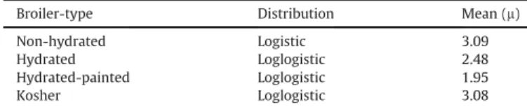
Weight of each broiler types in this PPP.
Broiler-type Distribution Mean (m)
Non-hydrated Logistic 3.09
Hydrated Loglogistic 2.48
Hydrated-painted Loglogistic 1.95
Kosher Loglogistic 3.08
Table 4
Distribution of the PPP production by chicken categories.
Process per day Not-hydrated Hydrated Hydrated-painted Kosher Probability Probability by process
1 100% e e e 11.1% 33.23% 1 e e e 100% 88.9% 2 45% e 55% e 70.0% 31.45% 2 80% e e 20% 30.0% 3 31% 23% 46% e 100.0% 32.58% 4 28% 27% 34% 11% 100.0% 2.74%
Steamton¼ b
b
0þ bb
1$LFOton ! þ bb
2$LFOtemp ! " bb
3$Airtemp ! þ bb
4$Watertemp ! " bb
5$FGtemp ! " bb
6$HeatLoss% ! " bb
7$%EfO2 ! (4)3.3.4. Meat meal plant (MMP)
Inedible offal contains about 27% of proteins used to produce meat meal. Dead broilers in farms and low-quality broilers from slaughtering increase the average of proteins to 33%. The meat meal yield is
m
¼ 30.33% (kg meal/kg waste), wherem
¼ 63.97% ispro-teins. A rotary drum screen filters the waste from slaughtering, where most of the solids are recovered and wastewater is sent to WTP. Process simulation was necessary to obtain the LCI data in this process due to the transformation of organic waste to a coproduct and air emissions. The model considered the characterization of inedible offal or organic matter (moisture, protein, fat, C, H, O, N, S, Cl and P) to carry out the simulation. Hydrolysis achieves the meal production.Fig. 4shows the endothermic reaction that takes place in the cooker or hydrolyzer. Since organic matter composition is complex, the coefficients (a-g) in the equation are unknown.
Emissions pass through an odor eliminator system where 60% of air emissions are reduced. A linear relationship, Eq. (5), was implemented to compute the process simulation results on MC.
yi¼ bix (5)
where y is the emission to be calculated, b is an index that expresses the amount of emission i generated for each unit of product x in the system, organic matter in this case.
3.3.5. Wastewater treatment plant (WTP)
The wastewater treatment followed a physical-chemical process until 2015 (seeFig. 5). This process consisted in a two-step capture of solid residues. The difference of densities between organic matter and water were used to separate solids in a holding tank. Then, the residues are decanted in clarification tanks, where wastewater treated and sludge are obtained. The efficiency of the global process was up to 65% (VSSout/VSSin).
In 2015, the WTP system was changed to a chemical-biological treatment (Fig. 6). The first step (a physical retention) eliminates 82% of solids; then, a dissolved air flotation unit removes solids. After that, nitrification-denitrification (aerobic treatment) process removes ammonium, and a biological reaction removes
phosphorus. Finally, a fluidized bed reactor is used to remove the residual suspended solids (sludge), using a polymer as a flocculant. Both cases were represented using a linear relationship on MC simulation (see Eq.(5)). Henceforth, system 1 will refer to farms operations plus PPP operations having a physical-chemical treat-ment (PPP1) in WTP; and system 2 will refer to farms operations plus PPP operations having a chemical-biological treatment (PPP2) in WTP.
3.3.6. Bioenergy production (sludge treatment plant, STP)
The sludge generated in WTP (system 1) was processed using anaerobic digestion, where biogas and bio-solids were obtained. Sludge characterization (physicochemical and biochemical) was defined using the results of laboratory analysis (1.02 ton/m3, 1.75%
w/w total solids or TS, 69% w/w total volatile solids or TVS). Before anaerobic digestion, a hydrolysis phase facilitated and enhanced the CH4generation, eliminating the bacteria that do not allow it. Fig. 7represents the overall process.
The biogas composition was 74.98% CH4, 25.02% CO2(v/v), while
biosolids showed a 57% of TVS removed.
In system 2, the sludge obtained has no methane potential because the aerobics conditions eliminate the bacteria that make possible biogas production. Hence, the sludge in system 2 is not anymore an input for another process, but a soil emission.
On MC simulation, the emissions were modeled as a linear relationship (see Eq.(5)).
Tables 5 and 6show the LCI obtained.
3.4. Impact assessment 3.4.1. Impact categories
Impacts were assessed following IMPACT 2002þ. This method classifies and expresses the emissions into reference substance (midpoints), making the interpretation simpler. Also, the midpoints categories are grouped into four types of damage categories (end-points), useful for optimization.
The midpoint categories are carcinogens (C), non-carcinogens (NC), respiratory inorganics (RI), ionizing radiation (IR), ozone layer depletion (OLD), respiratory organics (RO), aquatic ecotoxicity (AET), terrestrial ecotoxicity (TE), terrestrial acidification/nutrifi-cation (TA/N), land occupation (LO), aquatic acidifiacidification/nutrifi-cation (AA), aquatic eutrophication (AEU), global warming potential (GWP), non-renewable energy (NRE), and mineral extraction (ME).
Turning all emissions into midpoints is the first step of IMPACT 2002þ. Such a conversion is given by:
MPm¼X i X j " Emissionij$MFij# cm (6)
where i refers to each substance emitted to j (water, air or soil), m
Fig. 4. Representation of the meat meal production and the odors system.
represents each midpoint (MP) category, and MF is the midpoint factor. Once midpoints are calculated, Eq. (7) is used for deter-mining the damage categories (endpoints).
EPk¼X
m
ðMPm$EFkmÞ ck (7)
where k defines each endpoint (EP) category and EF is the endpoint factor. As each endpoint has a different unit of measurement, it is difficult to make a comparison between them. The set of normali-zation factors proposed by Jolliet et al. (2003) are applied to transform each category value into a new damage unit to overcome this problem. This new unit is called “point” (person,year), and represents the average impact in a specific category caused by a person during one year.
3.4.2. Allocation
The allocation process consists on partitioning the input or output flows of a unit process to the product system under study (ISO, 1997), measuring the individual impact for each product or by-product in the system. Most of the time, this step is avoided or underestimated in LCA studies.
Since there is more than one product in this PPP, impacts should be allocated to each product. For this purpose, three methods were evaluated. The first one is the classical mass method. In mass allocation, the allocation factor (AFMca) results by dividing the
number of product c (Pca), in a mass unit, by the total number of
products produced or output flows (OFa) in each area a:
AFM¼OFaPca ca;c (8)
This factor refers to the impact for each area; therefore, calcu-lating the total impact factor (AFMc) is necessary. AFMcis computed
as a weighted average of the factors previously calculated and the normalized impact units (pt) in each area a, divided by the total impact. Where k defines each endpoint category:
AFM¼ P a ! ðAFMÞ$"PkEPka #$ P kEPk cc (9)
In this case, the mass allocation has a drawback since energy is not measurable by a mass unit. Thus, sludge was selected to the mass allocation as sludge and energy production have a R2¼ 98.87%. This situation motivated the evaluation of Arti
ficial Neural Networks (ANN) and Stepwise Multivariate Regression (SMR) to allocate impacts without any restriction in units of measurement.
ANNs work through mathematical models that predict the behavior pattern of linear and non-linear systems. They consist of five main elements: normalized input values (xi), synaptic weights
(wij), bias (bi), an activation function (f), and the output value (y):
yo¼ f 0 @X j wij$xjþ bi 1 A (10)
ANNs are used to predict output values from independent var-iables, being useful in cases where the behavior is fluctuating and difficult to be predicted. Hyperbolic tangent function (tanh) was used in this case as activation function in a feedforward ANN with two layers (20 and 1 neurons respectively).
Weights (w) are “estimators” as in MLR, which determine the influence or importance of each input in the performance of the
Wastewater Soil emission
Rotary drum screen unit Eŋuent Solids Aerobic treatment / Phosphorus removal Fluidized bed reactor To conÞnement Sludge Water emission Chemical products Air emission Eŋuent Compressed air Return of sludge Soil emission
Fig. 6. Representation of the chemical-biological wastewater treatment.
Fig. 7. Representation of the anaerobic digestion process.
Table 5
Input data of the system per functional unit.
Inputs System 1 System 2 Unit
Al2O3 5.87E-04 0.00Eþ00 gr Ca(OH)2 0.07 0.06 gr Diesel 94.34 94.34 gr Electricity 0.13 0.13 kWh Energy (food) 48.46 48.46 MJ H2O 15.05 15.06 lt Heat (farms) 0.43 0.43 MJ
Light fuel oil 34.46 34.46 gr
LP gas 0.33 0.33 ml
N(l) 17.80 17.80 gr
NaCl 0.42 0.42 gr
NaClO 0.02 0.02 gr
NH3 0.02 0.02 gr
Packaging materials (PE) 0.24 0.24 gr
Packaging materials (PP) 0.15 0.15 gr
Protein 503.45 503.45 kg
Rice husk 1.36 1.36 kg
network. Therefore, they can be used to calculate the relative importance of each independent variable (seeGarson, 1991; Olden and Jackson, 2002). In this case, the relative importance is taken as the allocation factor for each product c (AFRc), calculated with:
AFR¼ P i . ðjwijj$jwiojÞ P jðjwijj$jwiojÞ / P jPi . ðjwijj$jwiojÞ P jðjwijj$jwiojÞ / cc (11)
where wij is the synaptic weight between the input j and the
neuron i, and wiois the synaptic weight between the neuron i, and
the output o.
SMR is a statistical technique used to calculate the regression values (estimators) when there are multiple values of input vari-ables. It consists of building a model by successively adding or removing variables based solely on the t-statistics of their esti-mated coefficients, i.e., variables with a poor contribution are removed from the model. Once b
b
j’s from Eq.(2)are calculated, theyare standardized (b
b
_j). This standardization uses the variationcaused by the output and input relation (Sxy), and the variation caused just by the output (Syy):
AFSc¼b
b
_j¼ bb
j$ 0S xy Syy 1 cc (12)The standardized value is taken as the allocation factor (AFSc)
since it represents the importance of inputs on the output value. In both cases (ANN and SMR), the coefficients (weights and estimators, respectively) are used as the basis for the allocation factors, due to their function in the models.
3.5. Multiobjective optimization 3.5.1. Genetic algorithms
GAs, developed by Holland in the 1970's, are search methods
based on the mechanisms of natural selection and principles of genetics. They are mathematical algorithms that transform a set of individual mathematical objects, using operations modeled ac-cording to the Darwinian-type survival-of-the-fittest strategy with sexual reproduction. Each object is usually a character string (let-ters or numbers) with a fixed-length adjusted to a chain of chro-mosomes. They are associated with a certain mathematical function that reflects its aptitude.
These strings represent parameters in the problem given; therefore, the natural evolution process is imitated to represent candidate solutions and to choose the best ones through compe-tition. The process is carried out by using three fundamental ge-netic operations: selection, crossover, and mutation.
In a multi-criteria problem, candidate solutions are found for a vector x! that minimize/maximize a set k of functions (Eq.(13)), for the decision vector given.
f ð x!Þ ¼ ½f1ð x!Þ;f2ð x!Þ;/; fkð x!Þ* (13)
A vector of constraints limiting the solution space affects every x value. These constraints can be represented as follows:
g1ð x!Þ + 0 (14)
h1ð x!Þ > 0 (15)
q1ð x!Þ ¼ 0 (16)
3.5.2. MCDA method
M-TOPSIS is a method for evaluation used to find a solution for multi-criteria problems (Ren et al., 2007), i.e., to find the best so-lution from the set of candidates. This soso-lution is the closest candidate to the ideal solution, which is the best in all criteria, and the farthest to the worst solution.
Table 6
Output data of the system per functional unit.
Outputs Unit System 1 System 2
Air Water Soil Air Water Soil
Ammonium N gr e e e e 1.40E-04 e
Ash gr 1.22E-02 2.98E-03 3.84Eþ00 1.22E-02 1.94E-04 6.28E-01
Biosolids gr e e 3.75Eþ01 e e e
Ca(OH)2 gr e 3.42E-04 e e 1.76E-06 5.67E-02
CFC (R22) gr 1.22E-03 e e 1.22E-03 e e
CH4 gr 8.63E-01 e e 8.63E-01 e e
CO2 gr 1.81Eþ02 e e 1.85Eþ02 e e
Fat gr 3.16E-02 2.23E-03 3.21Eþ00 3.18E-02 5.78E-05 1.87Eþ00
H gr 8.19Eþ00 e e 8.66Eþ00 e e
H2S gr e e e e e e
HCl gr 6.92E-02 8.56E-05 2.81E-06 7.12E-02 3.04E-06 9.82E-02
Hg gr e e 3.36E-04 e e e
K2O gr 9.61E-02 1.30E-04 2.90Eþ00 9.83E-02 4.89E-06 1.59E-01
Metals gr 3.97E-01 6.79E-04 2.04E-02 8.13E-01 1.87E-03 8.72E-01
N2O gr 1.58Eþ00 e e 1.58Eþ00 e e
NaCl gr e 1.53E-04 1.95E-01 e 1.16E-05 3.75E-01
NaClO gr e 1.64E-03 3.49E-06 e 4.20E-06 1.36E-01
NH3 gr 2.01Eþ01 e e 2.02Eþ01 e e
Ni gr e e 3.19E-03
NO3- gr e 5.90Eþ01 e e 5.90Eþ01 e
NOX gr 1.22E-01 e e 1.22E-01 e e
Organic waste gr e e 3.74Eþ01
P4O10 gr 3.98E-01 1.58E-03 7.56E-05 4.06E-01 5.66E-05 1.83Eþ00
PO43- gr e 2.88E-01 e e 2.88E-01 e
Poultry litter kg e e 2.72Eþ00 e e 2.72Eþ00
This solution can be found using Eq.(17). minfRig ¼ ffiffiffiffiffiffiffiffiffiffiffiffiffiffiffiffiffiffiffiffiffiffiffiffiffiffiffiffiffiffiffiffiffiffiffiffiffiffiffiffiffiffiffiffiffiffiffiffiffiffiffiffiffiffiffiffiffiffiffiffiffiffiffiffiffiffiffiffiffiffiffiffiffiffiffiffiffiffiffiffiffiffiffiffiffiffiffiffiffiffiffiffiffiffiffiffiffiffi ! Diþ""min3Diþ4#$2þ!Di"""max3Di"4#$2 q ci (17)
where Riis the distance between the solution i and the ideal
so-lution, Diþis the x value in the Cartesian plane corresponding to the
solution i, and Di-is the y value. Therefore, the ideal solution is in
(min{Diþ}, max{Di-}), determined from the set of candidates itself.
3.5.3. Mathematical model
Since system 1 is not operating nowadays, the optimization was only carried out for system 2. The optimization problem proposed in this study maximizes the income before taxes (revenue e costs) and minimizes the environmental impact of chicken meat pro-duction during one year.
The model determined which raw material or energy source should be used, and the number (mean) of each chicken type to be processed a day.
The basic operation was used to calculate the profit, as follows:
Profit ¼X C ðProdC$PricecÞ "X i ðQRMi$PriceRMiÞ "X j " QEj$PriceEj#" FC " VC (18)
The investment was not included, as new equipment is not required to increase the production or to change the raw material and energy sources. The variation between processes conditions was considered within fixed costs and variable costs.
The four endpoints categories of IMPACT 2002 þ are the envi-ronmental impacts to minimized. Thus, the mathematical model is:
Objective functions Maximize: Profit Minimize:
Human health (HH) Ecosystem quality (EQ) Climate change (CC) Resources (R) Subject to: a) Mass balance: X i X a RMiaþX j X a EjaþX c Ckncþ X c IIc ¼X c ProdcþX c FIcþX k X a Emka (19)
b) Production limits (lower and upper): Each type of carcass to be processed must be greater or equal to the market demand (considering the expected losses in the process) and less than the maximum production quantity historically obtained.
ðProdc*WcÞ*ð1 " ARLcÞ + MDc cc (20)
Prodc*Wc. MaxHc cc (21)
The sum of all products must be less than or equal to the ca-pacity of the plant:
X c
Prodc. PCap (22)
The coproducts production (ice, steam, etc.) must be greater than the needs of the main process and less than the capacities of the areas where processed, as follows:
X d CoProdd+ PReqd (23) X d CoProdd. SPCapd (24)
c) Requirements for raw materials and energy: to change the type of energy and raw materials at PPP, binary variables are used, where “0” equals to “not selected,” and “1” equals to “selected.” It is only possible to choose one option in each case; therefore, the sum must be 1:
X i
Gih¼ 1 ch (25)
Gih¼ ½0;1* ch (26)
The Gihthat has value 1 is the type i of energy h chosen to be
used in PPP. The decision variables are the number of chickens to be produced (four types), energy (fuel oil) to be used in boilers, energy (fuel gas) to use in different areas, and the type of refrigerant in cooling processes.where:
ARLcAverage rate of loss of carcass type c (dead or low-quality
chickens)
CkncChicken type c
CoProdcCoproduct type d
EMkaEmission type k in area a
EjaEnergy j used in area a
FC Fixed costs
FIcFinal inventory of carcass type c
GihType i of energy h
IIcInitial inventory of carcass type c
MaxHc Maximum production quantity historically obtained of
chicken c
MDcMarket demand for chicken type c
PCap PPP capacity
PReqdProcess requirements for coproduct d
PricecSale price of the processed carcass type c
PriceEjPrice of energy j
PriceRMiPrice of raw material i
ProdcCarcass of chicken type c
QEjQuantity of energy j
QRMiQuantity of raw material i
RMiaRaw material j used in area a
SPCapd Capacity for coproduct d VC Variable costs
WcWeight of chicken type c
4. Results and discussion 4.1. PPP products and coproducts
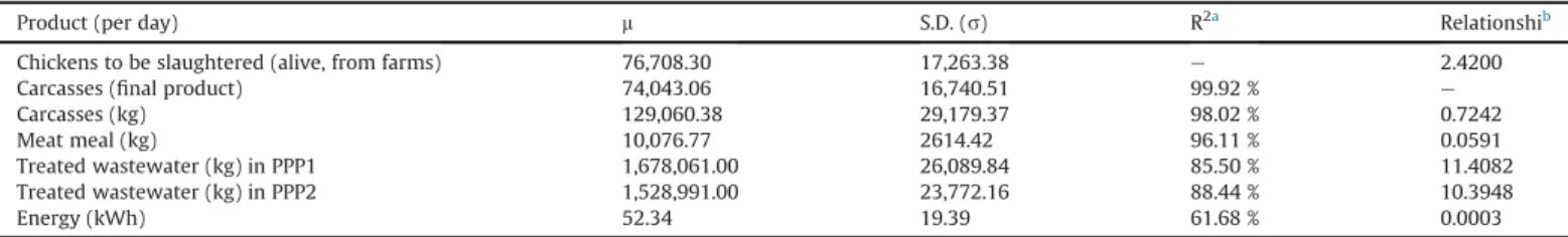
Table 7shows the products and coproducts obtained after MC runs. Standard Deviation (S.D.) is high due to the daily market demand.
4.2. Impact assessment
evaluation scores. TE is negative in chicken farms due to poultry litter. Poultry litter is the final residue on farms and consists of rice husk (bedding material), feces, urine, feathers and waste feed (Taupe et al., 2016). It contains proteins that benefit soil when discharged on it, but it is dangerous for environment and people because of pathogens.
Most of the impacts are the result of food extraction/production. Energy (food) impact ranges from 23% to 72%, while protein ranges from 12% to 44%. The highest impacts by food go to LO, TE, ME, C, GWP and AE due to all the necessary activities for obtaining food, from sowing, irrigation, fertilization and pest control to harvesting, affecting all midpoints by over 75%. Poultry manure has a consid-erable contribution in IR (35%). Poultry manure used as fertilizer or animal food releases CH4contributing to the ozone layer depletion
(19%). In other categories, it has an impact less than 19%. Shed impact is not bigger than 0.01%, and hence it could be omitted in future evaluations. Heat generation impact is low in each category because of the relative temperature in Mexico. High outside
temperatures cause a minor use of fuels to produce necessary heat in the first few weeks on farms; therefore, countries with a low outside temperature need more fuel to operate. However, impacts due to energy and heat production are low in farms activities.
On-farm emissions are responsible for 24% RI, 58% TAN, 63% AA and 3% GWP, because of ammonia mainly. NH3(14 gr$kg LW-1) is
produced by the putrefaction of the nitrogenous matter coming from plants and animals. It is not dangerous for humans, but for aquatic animals. N2O and CH4are released in this process but minor
quantities.
Slaughterhouse activities have a considerable impact in NC, OLD, RO, and AEU. NC is caused by organic waste, hydrolyzed in MMP and emitted to water in WWTP. RO has the same origin, combustion of organic waste (60%), including blood and feathers. PPP contrib-utes to OLD by steam production (CO2and SO2and NOx emissions)
and NH3lost in the ice production and cooling chambers due to the
draining process.
AEU is originated by chicken scalding mainly, where chickens are immersed into hot water to remove feather. The process implies a P and COD emission as reported byGonz!alez-Garcia et al. (2014). In system 1, AEU is also due to a large amount of organic waste are sent to rivers since the physical-chemical process is not enough to remove all contaminants. The impact to AEU is similar in system 2 due to sludge is not anymore used to produce energy, but confined, affecting underground water.
The use of packaging materials has been optimized in the last few years, resulting in a low impact compared to other works in literature.
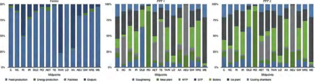
Fig. 9shows these data, dividing farms into four groups: feed production, energy production, facilities and outputs; and PPP in
Table 7 PPP production.
Product (per day) m S.D. (s) R2a Relationshib
Chickens to be slaughtered (alive, from farms) 76,708.30 17,263.38 e 2.4200
Carcasses (final product) 74,043.06 16,740.51 99.92 % e
Carcasses (kg) 129,060.38 29,179.37 98.02 % 0.7242
Meat meal (kg) 10,076.77 2614.42 96.11 % 0.0591
Treated wastewater (kg) in PPP1 1,678,061.00 26,089.84 85.50 % 11.4082
Treated wastewater (kg) in PPP2 1,528,991.00 23,772.16 88.44 % 10.3948
Energy (kWh) 52.34 19.39 61.68 % 0.0003
aDetermination coefficient related to kg LW chicken to be slaughtered. b Product in kg or kWh obtained per 1 kg LW chicken to be slaughtered.
Table 8
Environmental impact of chicken meat production per FU (characterization).
Midpoint System 1a System 2b Unit Endpoint
Mean S.D. Mean S.D.
C 0.0597 0.0123 0.0604 0.0125 kg C2H3Cl eq HH
NC "0.0061 0.0021 "0.0032 0.0020 kg C2H3Cl eq HH
RI 0.0059 0.0013 0.0059 0.0013 kg PM2.5eq HH
IR 23.2129 4.4610 23.3995 4.5118 Bq C-14 eq HH
OLD 1.87E-07 2.31E-07 1.87E-07 2.32E-08 kg CFC-11 eq HH
RO 0.0032 0.0008 0.0032 0.0008 kg C2H4eq HH AE 142.1902 29.5487 141.5938 29.4463 kg TEG water EQ TE "113.2558 26.7685 "102.5666 24.8868 kg TEG soil EQ TA/N 0.4124 0.0932 0.4127 0.0933 kg SO2eq EQ LO 3.8377 0.8773 3.8377 0.8773 m2org.arable EQ AA 0.0540 0.0136 0.0544 0.0137 kg SO2eq EQ AEU 0.0045 0.0013 0.0055 0.0016 kg PO4P-lim EQ GWP 2.7729 0.5818 2.7928 0.5870 kg CO2eq CC NRE 32.2122 5.6642 32.5003 5.7360 MJ primary R ME 0.1093 0.0228 0.1087 0.0228 MJ surplus R
aSystem 1: farms þ PPP with a physical-chemical treatment in WTP. b System 2: farms þ PPP with a chemical-biological treatment in WTP.
Table 9
Environmental impact of chicken meat production per FU (evaluation).
Endpoint System 1 System 2 Unit
Mean S.D. Mean S.D.
HH 4.2720E-06 9.2666E-07 4.2953E-06 9.3262E-07 DALYa
EQ 3.7232 0.8431 3.8081 0.8634 PDF,m2
,yrb
CC 2.7730 0.5818 2.7928 0.5870 kg CO2eq
R 32.3251 5.6868 32.6090 5.7587 MJ primary
aDisability-adjusted life years.
seven groups: slaughtering, MMP, WTP, STP, boilers, ice plant and cooling chambers.
Considering all these data, it is evident that changing from a physical-chemical to a chemical-biological process in WTP caused an adverse environmental impact, due to three reasons mainly: a higher electric energy demand, non-bioenergy production from sludge, and untreated sludge. Sludge was digested to produce en-ergy from biogas combustion (PPP1). This enen-ergy was used to po-wer the ice plant; therefore, once methane production was not possible anymore, PPP had to obtain the energy from the public network again increasing the environmental impact. However, a chemical-biological process usually reduces water contamination when correctly implemented.
The new WTP process requires over 19% more electricity. The increase in energy requirement is due to the new machinery operating in the process. Thus, the electrical energy demand is 3.64 Wh/kg treated water for system 2, and 2.79 Wh/kg for system 1.
According to Ecoinvent, producing 1 kWh causes 0.647 kg CO2e
and needs 10.897 MJ in Mexico.
The little improvement in AET, OLD and ME is due to a lower consumption of chemicals in the wastewater treatment, since the stages in the new WWTP induce natural processes.
NRE (þ0.49%), GWP (0.34%) are affected by the increment in the energy demand due to WWTP and ice plant, þ0.6% and þ1.3% of the total consumption respectively.
Sludge quality is different for system 1 and 2. In system 1, sludge is obtained from a high chemical application (5.87 / 10-4gr Al2O3
FU-1, mainly) affecting to RI, GWP, and NRE due to its extraction and production. However, wastewater has a high content of organic waste that increments BOD and COD. In system 2, the use of chemicals and emissions are reduced significantly, but NH3-N and
NO3- are released by the nitrification/denitrification process,
increasing 0.60% AA impact. The resulting sludge is not treated, but it is a direct emission; therefore, proteins and organic waste are not transformed into energy.
In PPP 1, boilers and ice plant impacts represent almost the 67% of the whole PPP, while WTP represents less than 2%. The reason is that WTP waste affects just to water, and solid residues (sludge) were treated in STP. In boilers, LFO (34.46 g LFO/FU) is the main contributor to the environmental impact (0.53 kg CO2e and
57.32 MJ per LFO), followed by emissions to air (105.96 g CO2, 2.15 g
SO2, and 0.091 g NOx per FU).
In PPP 2, the impact of boilers and ice plant reduced to 65%, caused by the increment in WTP impact (4.09%) mentioned above (more energy requirement and solid residues or sludge not treated.).
Thus, farms cause 84.86% and 84.04% of environmental impacts, and only 15.14% and 15.96% is due to PPP, respectively for system 1 and 2 (based on normalized data from one year's production in MC simulation). The difference between farms and PPP is due to a large amount of time required in farms (5e7 weeks) to get the desired weight, against the quick process in PPP (0.33 h for NHy type, 1.17 h Hy and HyP types, and 2 h for Kr type).
The R2among endpoints is above 99%. For all the 15 midpoint
categories, the R2value goes from 26% to 99%. AET, LO, NC-ME and LO-NC-ME categories present the highest value (>98%), while RO-EM presents the lowest value (26.03%).
The difference between inputs and outputs impact at the PPP is lower but significant. Inputs cause 77.85% and 75.52% of the PPP impact, while output causes only 22.15% and 24.48%, respectively.
Considering the endpoint scores, HH receives the greatest impact because of its normalization factor (Jolliet et al., 2003). Resources receive the least impact, while EQ and CC are statistically equal. InFig. 8are these values represented per FU.
4.3. Allocation
The impact due to farms operation is the same for each indi-cator: 41.26% for NHy, 23.12% for Hy, 34.77% for HyP, and 0.85% for Kr (only was mass method applied); since the only difference be-tween chicken types is the time to get the final weight. Therefore, results in this section only focuse on PPP impact.
The behavior of the allocation factors is similar in all three cases (seeFig. 10). Since PPP production varies every day, these indicators were calculated using data from one year's production in MC. NHy chicken causes the highest weight because it is the product with the highest production and weight.
These results can be used for the final impacts presented in
Tables 8 and 9Following this, every product and coproduct has the same impact in each indicator (as in farms), so impact allocation by area is needed. Even though ANN and regression have no restriction in using any measurement unit, it is complicated to obtain the specific weights for each area because they require many mathe-matical calculations.
Fig. 11 shows the allocation distribution for each indicator, following the mass method only. The only midpoint that changed significantly is NC caused by the denitrification/nitrification stage in the new WTP (NH3-N emissions). However, as presented in Tables 8 and 9, all impacts increased in system 2, except for AE, that improved in 0.42% per FU due to a better wastewater quality, i.e., the new WTP process was not a wrong decision, but planned incorrectly.
Fig. 8. MC simulation results per FU for each endpoint in both systems, based on normalized values (1 pt ¼ 1000 mpt).
Fig. 11also shows that STP impact is just above 0% in system 1, as bioenergy production system only uses sludge for methane gen-eration and a very small amount of energy for small pumps operation.
4.4. Comparison with previous studies
A comparison with previous LCA studies involving broiler chicken was conducted to determine the performance of this pro-cess where “1 kg carcass” is used as FU.
As reported in the literature (Bengtsson and Seddon, 2013; da Silva et al., 2014; Gonz!alez-Garcia et al., 2014), farms contribute the most to environmental impacts, being feed production the largest contributor. It could be due to many factors, for example, chemicals used as fertilizers and pesticides, as well as the defor-estation inherent to the crop. On-farm emissions result by organic waste (rice husk, feed, feces, feathers, etc.) decomposition. The decomposition generates NH3, NO3-, PO43-and CH4emissions.
This study found that slaughterhouse stage contributes the most only in three categories: OLD (56.59%), RO (67.08%) and AEU (71.98%), due to wastewater, and fuel oil combustion for steam production.
Fig. 12shows a comparison between this study and other five, using AA, AEU, GWP and Cumulative Energy Demand (CED) in-dicators (CED ¼ R), quantifying the uncertainty and variability ef-fect on the results. These five studies were selected due to the similar FU and system boundaries used. In some cases, minor cal-culations were required.
The comparison was conducted using only system 2 since sys-tem 1 is not operating.
In AA, this case study (0.05 kg SO2e FU"1) is considerably lower
than the value reported inWilliams et al. (2006) but equals to
Gonz!alez-Garcia et al. (2014)andda Silva et al. (2014).
AA is caused by SO2, which is released in combustion process as
fuel oil, diesel, and gases. The use of fuel oil in boilers is high for this case study, so special attention must be paid to the S concentration. Concerning AEU, this case study shows a good performance even with a “bad” wastewater treatment, since AEU is a direct result of wastewater discharges. AEU ranges from 0.02 to 0.05 kg PO4e
FU"1in the literature (da Silva et al., 2014; Gonz!alez-Garcia et al., 2014; Williams et al., 2006).
GWP is the most used indicator to make a comparison between studies. GWP ranges from 1.39 to 3.12 kg CO2e kg-1LW only on-farm
activities (Baumgartner et al., 2008; Bengtsson and Seddon, 2013; da Silva et al., 2014; Gonz!alez-Garcia et al., 2014; Katajajuuri, 2007; Leinonen et al., 2012; Pelletier, 2008), while this study re-ported 1.58 kg CO2e kg-1 LW. There are several reasons for this
variation, one of them is the method of farming that could be free-range, standard indoor or organic production. Data quality, feed and bed composition and waste handling contribute to this variation too. In this case study, poultry bed is made of rice husk, but other studies report the use of wood and bagasse. Poultry litter could be used for different applications, for example, organic fertilizer and animal feed, avoiding the production of an equivalent amount of these products (Pelletier, 2008).
Regarding slaughterhouse, GWP ranges from 0.5 to 1.11 kg CO2e
Fig. 10. Comparison of the allocation factors from the three proposed methods (Mass method, ANN, and SMR) for the PPP-related operations only, calculated as their relative importance.
Fig. 11. Midpoints allocation (in %) by PPP coproduct, based on non-normalized values from one year's production in MC
Fig. 12. Comparison between similar case studies (cradle-to-PPP gate approach) per FU, showing ranges of uncertainty (min-max) for this case study. (Values are normalized based on the results of this case study).
FU"1(da Silva et al., 2014; Gonz!alez-Garcia et al., 2014). This study
reports 1.21 kg CO2e FU"1which is high compared to literature. This
is caused by the high steam demand by the MMP being 66% of the total PPP demand. The more the steam production, the more the emissions by fuel combustion. This is the main reason for the GWP difference since no works have reported a similar stage in their poultry chain (system boundaries).
According to The World Bank, in 2011, CO2e emissions were 3.9
tons per capita in Mexico, which means that this case study has the same annual impact in CC than 28,247 Mexicans. In energy metrics, the impact of this case study (in R) is equivalent to the impact of 20,018 Mexicans (63.86 GJ per capita).
Energy demand is another good reference for the performance of the production chain. Focusing only on chicken farms, CED ranges from 14.96 to 34.80 MJe FU"1while taking into account slaughterhouse makes this indicator to increase to 18.5e65.04 MJe. Since all of the raw materials need energy to be extracted and processed, this indicator depends directly on the agricultural, mining and energy production practices. Mexico produces most of its food, and this case study uses only local products, resulting in a low energy demand (32.61 MJ FU"1). The high steam demand in
this PPP also affects to CED.
Finally, LO could be used to compare chicken production in farms because of food production. This value ranges from 3.9 m2to 4.9 m2$kg LW-1(Baumgartner et al., 2008; Leinonen et al., 2012), while this case found 2.67 ± 0.87 m2$kg LW-1. This difference is due to the chicken diet and the food availability near farms.
In all cases, the results depend on the country in which studies were developed and on the assumptions for data collection (liter-ature, surveys, collection in situ, simulation, and so on), in addition to those reasons mentioned above.
Regarding the system boundaries definition, this case study includes key stages in the PPP, a process like steam production, MMP, and ice production, not mentioned in other works, but it is assumed that at least steam production or its equivalent was taken into account.
4.5. Optimization
The last step of the proposed methodology tries to figure out the
scenario in which the income before taxes and the environmental impact of chicken meat production are optimized at the same time. GAs were applied to a mathematical model described in section
3.5.3 through MultiGen®
library. The NSGA-II Full-continuous mixed algorithm was used with the following parameters: in-dividuals in the population ¼ 400; number of generations ¼ 200; crossover rate ¼ 0.9; mutation rate ¼ 0.5.
For the Pareto front, 41 values (candidates) were generated and analyzed using M-TOPSIS. Fig. 13 shows the graphics of Pareto fronts, where each environmental indicator against profit (most important objective for the PPP's CEO) is compared. This figure also shows the solutions for the mono-criterion problems (profit as FO), which was carried out for comparison.
The best alternative results in HH ¼ 4349 pt, EQ ¼ 841 pt, CC ¼ 2997 pt, and R ¼ 3978 pt (PPP impact only) from one year's production in MC. This result is achieved by distribution the PPP production as follows: NHy ¼ 36,316; Hy ¼ 35,986; HyP ¼ 37,694; and Kr ¼ 0 chickens a day, on average. This result in manly due to the good prices of Hy and HyP types.
Fig. 13. Pareto fronts in two dimensions (profit vs. environmental indicators). The best solution to multi-criteria problems is represented by a black dot, while the best so-lution for mono-criterion optimization is represented in red. The results figure is not the typical one because of the small number of non-dominated solutions.
Fig. 14. Relative contributions (in %) from the stages considered in this study, farms, and slaughterhouse (or PPP), based on normalized values from one year's production in MC.
Fig. 15. Relative contributions (in %) from inputs and outputs at PPP (impact caused by raw material and energy requirements vs. impact caused by emissions), based on normalized values from one year's production in MC.
For energy sources, using LFO instead of the traditional Heavy type is recommended due to a lower GWP (0.527 vs. 0.464 kg CO2e
per kg fuel) and a lower sulfur content in LFO (3% vs. 4%). A reduction of emissions of SO2to the atmosphere ("33% per FU) is
obtained while having a good performance in the process. When using HFO, RI and TAN increase 25% in boilers.
Natural gas should be used in other areas instead LP gas to heat generation and as a fuel for machinery (forklifts) due to a lower energy demand (54.04 vs. 58.23 MJ per kg gas) and GWP (0.587 vs. 0.494 kg CO2e per FU). LP gas combustion released a greater
amount of CO2because of its higher C content.
Tetrafluoroethane (CH2FCF3) is recommended as a refrigerant in
the cooling processes as it is less aggressive to ozone layer that the current CHClF2. CFC's can be present in the atmosphere from 50 to
100 year once emitted, damaging the ozone layer because of the presence of Cl. That is why they are not allowed in some countries anymore. Production of CHClF2implies 29.41 kg CO2e and 95.07 kg
Bq C-14, against 3.10 kg CO2e and 55.33 kg Bq C-14 related to
CH2FCF3.
It is also possible to improve IQF process, changing the actual system (nitrogen immersion) to a compression refrigeration using NH3, which would reduce the cost to 90% approximately, and the environmental impact due to the recirculation of refrigerant. This possibility is not addressed in the optimization because of the necessary economic investment.
Since Kr-type has special requirements and is not processed regularly, the algorithm gives a value of zero. The value suggests that the kosher production must be removed from PPP. However, this is not possible due to an arrangement between PPP manage-ment and Jewish people.
For this new production, the impact increased to 12,165 in the PPP, in addition to the farm impact not considered for optimization that increased to 77 Mpt$year-1.
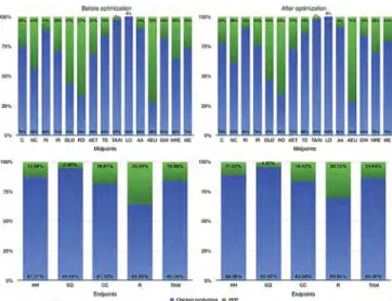
The graphics inFig. 14show the comparison between farms and PPP impact before and after optimization (based on normalized data from one year's production in MC). Chicken production (farms) causes 84% (before optimization) and 86% (after optimization) of the total environmental impacts. Inputs and outputs of PPP are compared inFig. 15; inputs cause 76% (before optimization) and 74% (after optimization) of the impacts.
Compared with the current system, the improvement is remarkable. The PPP impact passed from 15.96% to 13.64% of the total system. Emissions caused by inputs decreased from 75.52% to 73.67% due to the change in the use of energy and raw materials. The reduction represents an improvement of 0.64% per FU from cradle to PPP gate (1.3803e1.3714 mpt$FU"1), and 15.14% from
farms gate to PPP gate (0.2204e0.1870 mpt$FU"1).
Table 10presents the reduction in each midpoint, where NC was the most benefited impact reaching an improvement of 41%. Considering only the PPP impact, ME is the most benefited impact with an improvement of 25%.
5. Conclusions
This paper proposes an integrated framework based on LCA methodology to evaluate the environmental impacts of chicken meat production. In this framework, LCA is coupled with simulation
and artificial intelligence techniques to expand the perspective and scope beyond the LCA limits. The simulation was used to propagate variability, uncertainty, and complexity into LCA results, while ge-netic algorithms allowed a multiobjective optimization (impact minimization and profit maximization).
This approach was applied in a Mexican case study from cradle to PPP gate. Results show that the surrounding systems cause a bigger impact than the transformation process itself, as reported in the literature. Chicken farms were identified as the main contrib-utors, which is caused by feed production and on-farm emissions mainly. Concerning the PPP, the steam production in boilers and ice production cause most of the impact due to energy and refrigerants requirements. Allocations methods showed a significant difference, but a high correlation. The NHy broiler type is the product with the highest impact in all three methods tested. Mass method is used to report results since ANN and SMR results are used to allocate final impacts only, but not by areas, allocating to be constant in every midpoint. This could be solved by applying ANN and SMR by area in future works.
This case showed a performance within the international ranges when compared with previous studies. However, differences in location, characteristics of the processes and data collection must be taken into account.
The best alternative in the multiobjective optimization showed an impact reduction by 15.14% per kg carcass. This reduction is possible for a better distribution of production, and a better choice of energy and raw materials used.
Thus, this paper presents a novel approach to LCA studies, since it expands the perspective beyond the LCA limits, and provides a more holistic picture of the system. This could be interesting for both the environmental sector and the chicken sector.
Acknowledgments
Authors are grateful to CONACYT (the Mexican National Council of Science and Technology) for the support received in the Master thesis, which was the base of this work, and to the PPP manage-ment for allowing the data collection in its facilities.
References
Alexander, B., Barton, G., Petrie, J., Romagnoli, J., 2000. Process synthesis and optimisation tools for environmental design: methodology and structure. Comput. Chem. Eng. 24 (2-7), 1195e1200.
Amudha, A., Vijayalakshmi, V.J., Sugumaran, G., 2015. Single-objetive optimization of profit and emission under deregulated environment. Procedia Technol. 21, 400e405.
Basset-Mens, C., van der Werf, H., Durand, P., Leterme, P., 2006. Implications of uncertainty and variability in the life cycle assessment of pig production sys-tems. Int. J. LCA 11 (5), 298e304.
Baumgartner, D.U., de Baan, L., Nemecek, T., 2008. European Grain Legu-meseEnvironment-friendly Animal Feed. Life Cycle Assessment of Pork, Chicken Meat, Egg and Milk Production. Grain Legumes Integrated Project. Report. Agroscope Reckenholz-T€anikon Research Station ART, Zürich.
Bengtsson, J., Seddon, J., 2013. Cradle to retailer or quick service restaurant gate life cycle assessment of chicken products in Australia. J. Clean. Prod. 41, 291e300.
Bieda, B., 2014. Application of stochastic approach based on Monte Carlo (MC) simulation for life cycle inventory (LCI) to the steel process chain: case study. Sci. Total Environ. 481, 649e655.
Brunet, R., Cort!es, D., Guill!en-Gos!albez, G., Jim!enez, L., Boer, D., 2012. Minimization of the LCA impact of thermodynamic cycles using a combined simulation-optimization approach. Appl. Therm. Eng. 48, 367e377.
Table 10
Reduction by midpoints (values before optimization were taken as 100%).
C NC RI IR OLD RO AET TE TA/N LO AA AEU GW NRE ME
In system 2 99% 59% 100% 96% 94% 96% 96% 94% 98% 98% 86% 88% 99% 95% 95%