Retouched Bloom Filters:
Allowing Networked Applications to Trade Off
Selected False Positives Against False Negatives
Benoit Donnet
Univ. Catholique de Louvain
Bruno Baynat
Univ. Pierre et Marie Curie
Timur Friedman
Univ. Pierre et Marie Curie
ABSTRACT
Where distributed agents must share voluminous set mem-bership information, Bloom filters provide a compact, though lossy, way for them to do so. Numerous recent networking papers have examined the trade-offs between the bandwidth consumed by the transmission of Bloom filters, and the er-ror rate, which takes the form of false positives, and which rises the more the filters are compressed. In this paper, we introduce the retouched Bloom filter (RBF), an extension that makes the Bloom filter more flexible by permitting the removal of selected false positives at the expense of gen-erating random false negatives. We analytically show that RBFs created through a random process maintain an overall error rate, expressed as a combination of the false positive rate and the false negative rate, that is equal to the false positive rate of the corresponding Bloom filters. We further provide some simple heuristics that decrease the false posi-tive rate more than than the corresponding increase in the false negative rate, when creating RBFs. Finally, we demon-strate the advantages of an RBF over a Bloom filter in a dis-tributed network topology measurement application, where information about large stop sets must be shared among route tracing monitors.
Categories and Subject Descriptors
C.2.1 [Network Architecture and Design]: Network Topology; E.4 [Coding and Information Theory]: Data Compaction and Compression
General Terms
Algorithms, Performance
Keywords
Bloom filters, false positive, false negative, bit clearing, measurement, traceroute
Permission to make digital or hard copies of all or part of this work for personal or classroom use is granted without fee provided that copies are not made or distributed for profit or commercial advantage and that copies bear this notice and the full citation on the first page. To copy otherwise, to republish, to post on servers or to redistribute to lists, requires prior specific permission and/or a fee.
CoNEXT2006, Lisbon, Portugal
Copyright 2006 ACM 1-59593-456-1/06/0012 ...$5.00.
1.
INTRODUCTION
The Bloom filter is a data structure that was introduced in 1970 [1] and that has been adopted by the networking research community in the past decade thanks to the band-width efficiencies that it offers for the transmission of set membership information between networked hosts. A sender encodes the information into a bit vector, the Bloom filter, that is more compact than a conventional representation. Computation and space costs for construction are linear in the number of elements. The receiver uses the filter to test whether various elements are members of the set. Though the filter will occasionally return a false positive, it will never return a false negative. When creating the filter, the sender can choose its desired point in a trade-off between the false positive rate and the size. The compressed Bloom filter, an extension proposed by Mitzenmacher [2], allows further bandwidth savings.
Broder and Mitzenmacher’s survey of Bloom filters’ net-working applications [3] attests to the considerable interest in this data structure. Variants on the Bloom filter con-tinue to be introduced. For instance, Bonomi et al.’s [4] d-left counting Bloom filter is a more space-efficient version of Fan et al.’s [5] counting Bloom filter, which itself goes be-yond the standard Bloom filter to allow dynamic insertions and deletions of set membership information. The present paper also introduces a variant on the Bloom filter: one that allows an application to remove selected false positives from the filter, trading them off against the introduction of random false negatives.
This paper looks at Bloom filters in the context of a net-work measurement application that must send information concerning large sets of IP addresses between measurement points. Sec. 5 describes the application in detail. But here, we cite two key characteristics of this particular applica-tion; characteristics that many other networked applications share, and that make them candidates for use of the variant that we propose.
First, some false positives might be more troublesome than others, and these can be identified after the Bloom filter has been constructed, but before it is used. For in-stance, when IP addresses arise in measurements, it is not uncommon for some addresses to be encountered with much greater frequency than others. If such an address triggers a false positive, the performance detriment is greater than if a rarely encountered address does the same. If there were a way to remove them from the filter before use, the applica-tion would benefit.
negatives. It would benefit from being able to trade off the most troublesome false positives for some randomly intro-duced false negatives.
The retouched Bloom filter (RBF) introduced in this pa-per pa-permits such a trade-off. It allows the removal of se-lected false positives at the cost of introducing random false negatives, and with the benefit of eliminating some random false positives at the same time. An RBF is created from a Bloom filter by selectively changing individual bits from 1 to 0, while the size of the filter remains unchanged. As Sec. 3.2 shows analytically, an RBF created through a ran-dom process maintains an overall error rate, expressed as a combination of the false positive rate and the false negative rate, that is equal to the false positive rate of the corre-sponding Bloom filter. We further provide a number of sim-ple algorithms that lower the false positive rate by a greater degree, on average, than the corresponding increase in the false negative rate. These algorithms require at most a small constant multiple in storage requirements. Any additional processing and storage related to the creation of RBFs from Bloom filters are restricted to the measurement points that create the RBFs. There is strictly no addition to the critical resource under consideration, which is the bandwidth con-sumed by communication between the measurement points. Some existing Bloom filter variants do permit the suppres-sion of selected false positives, or the removal of information in general, or a trade-off between the false positive rate and the false negative rate. However, as Sec. 6 describes, the RBF is unique in doing so while maintaining the size of the original Bloom filter and lowering the overall error rate as compared to that filter.
The remainder of this paper is organized as follows: Sec. 2 presents the standard Bloom filter; Sec. 3 presents the RBF, and shows analytically that the reduction in the false pos-itive rate is equal, on average, to the increase in the false negative rate even as random 1s in a Bloom filter are re-set to 0s; Sec. 4 presents several simple methods for selec-tively clearing 1s that are associated with false positives, and shows through simulations that they reduce the false positive rate by more, on average, than they increase the false negative rate; Sec. 5 describes the use of RBFs in a network measurement application; Sec. 6 discusses several Bloom filter variants and compares RBFs to them; finally, Sec. 7 summarizes the conclusions and future directions for this work.
2.
BLOOM FILTERS
A Bloom filter [1] is a vector v of m bits that codes the membership of a subset A = {a1, a2, . . . , an} of n elements
of a universe U consisting of N elements. In most papers, the size of the universe is not specified. However, Bloom filters are only useful if the size of U is much bigger than the size of A.
The idea is to initialize this vector v to 0, and then take a set H = {h1, h2, . . . , hk} of k independent hash functions
h1, h2, . . . , hk, each with range {1, . . . , m}. For each element
a∈ A, the bits at positions h1(a), h2(a), . . . , hk(a) in v are
set to 1. Note that a particular bit can be set to 1 several times, as illustrated in Fig. 1.
In order to check if an element b of the universe U belongs to the set A, all one has to do is check that the k bits at positions h1(b), h2(b), . . . , hk(b) are all set to 1. If at least
one bit is set to 0, we are sure that b does not belong to
h1(b) h2(b) h2(a) h1(a) 1 0 0 1 0 0 1 0 0 0
Figure 1: A Bloom filter with two hash functions
U
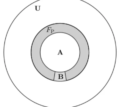
A
B FP
Figure 2: The false positives set
A. If all bits are set to 1, b possibly belongs to A. There is always a probability that b does not belong to A. In other words, there is a risk of false positives. Let us denote by FP the set of false positives, i.e., the elements that do not
belong to A (and thus that belong to U − A) and for which the Bloom filter gives a positive answer. The sets U , A, and FP are illustrated in Fig. 2. (B is a subset of FP that will
be introduced below.) In Fig. 2, FP is a circle surrounding
A. (Note that FPis not a superset of A. It has been colored
distinctly to indicate that it is disjoint from A.)
We define the false positive proportion fP as the ratio of
the number of elements in U −A that give a positive answer, to the total number of elements in U − A:
fP =
|FP|
|U − A| (1)
We can alternately define the false positive rate, as the probability that, for a given element that does not belong to the set A, the Bloom filter erroneously claims that the element is in the set. Note that if this probability exists (a hypothesis related to the ergodicity of the system that we assume here), it has the same value as the false positive proportion fP. As a consequence, we will use the same
no-tation for both parameters and also denote by fP the false
positive rate. In order to calculate the false positive rate, most papers assume that all hash functions map each item in the universe to a random number uniformly over the range {1, . . . , m}. As a consequence, the probability that a specific bit is set to 1 after the application of one hash function to one element of A is 1
m and the probability that this specific
bit is left to 0 is 1 − 1
m. After all elements of A are coded in
the Bloom filter, the probability that a specific bit is always equal to 0 is p0 = „ 1 − 1 m «kn (2) As m becomes large, 1
m is close to zero and p0 can be
approximated by
p0 ≈ e−
kn
m (3)
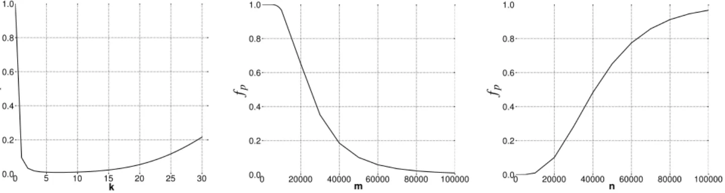
Figure 3: fP as a function ofk, m and n.
expressed as
p1 = 1 − p0 (4)
The false positive rate can then be estimated by the prob-ability that each of the k array positions computed by the hash functions is 1. fP is then given by
fP = pk1 = “1 −`1 − 1 m ´kn”k ≈ “1 − e−knm ”k (5)
The false positive rate fP is thus a function of three
pa-rameters: n, the size of subset A; m, the size of the filter; and k, the number of hash functions. Fig. 3 illustrates the variation of fPwith respect to the three parameters
individ-ually (when the two others are held constant). Obviously, and as can be seen on these graphs, fPis a decreasing
func-tion of m and an increasing funcfunc-tion of n. Now, when k varies (with n and m constant), fP first decreases, reaches
a minimum and then increases. Indeed there are two con-tradicting factors: using more hash functions gives us more chances to find a 0 bit for an element that is not a member of A, but using fewer hash functions increases the fraction of 0 bits in the array. As stated, e.g., by Fan et al. [5], fPis
minimized when
k = mln 2
n (6)
for fixed m and n. Indeed, the derivative of fP (estimated
by eqn. 3) with respect to k is 0 when k is given by eqn. 6, and it can further be shown that this is a global minimum. Thus the minimum possible false positive rate for given values of m and n is given by eqn. 7. In practice, of course, kmust be an integer. As a consequence, the value furnished by eqn. 6 is rounded to the nearest integer and the resulting false positive rate will be somewhat higher than the optimal value given in eqn. 7.
ˆ fP = „ 1 2 «m ln 2n ≈ (0.6185)mn (7)
Finally, it is important to emphasize that the absolute number of false positives is relative to the size of U − A (and not directly to the size of A). This result seems surprising as the expression of fP depends on n, the size of A, and does
not depend on N , the size of U . If we double the size of U− A (and keep the size of A constant) we also double the
absolute number of false positives (and obviously the false positive rate is unchanged).
3.
RETOUCHED BLOOM FILTERS
As shown in Sec. 2, there is a trade-off between the size of the Bloom filter and the probability of a false positive. For a given n, even by optimally choosing the number of hash functions, the only way to reduce the false positive rate in standard Bloom filters is to increase the size m of the bit vector. Unfortunately, although this implies a gain in terms of a reduced false positive rate, it also implies a loss in terms of increased memory usage. Bandwidth usage becomes a constraint that must be minimized when Bloom filters are transmitted in the network.
3.1
Bit Clearing
In this paper, we introduce an extension to the Bloom filter, referred to as the retouched Bloom filter (RBF). The RBF makes standard Bloom filters more flexible by allow-ing selected false positives to be traded off against random false negatives. False negatives do not arise at all in the standard case. The idea behind the RBF is to remove a certain number of these selected false positives by resetting individually chosen bits in the vector v. We call this pro-cess the bit clearing propro-cess. Resetting a given bit to 0 not only has the effect of removing a certain number of false positives, but also generates false negatives. Indeed, any element a ∈ A such that (at least) one of the k bits at posi-tions h1(a), h2(a), . . . , hk(a) has been reset to 0, now triggers
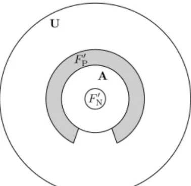
a negative answer. Element a thus becomes a false negative. To summarize, the bit clearing process has the effects of decreasing the number of false positives and of generating a number of false negatives. Let us use the labels F′
Pand FN′
to describe the sets of false positives and false negatives after the bit clearing process. The sets F′
P and FN′ are illustrated
in Fig. 4.
After the bit clearing process, the false positive and false negative proportions are given by
f′ P = |F′ P| |U − A| (8) f′ N = |F′ N| |A| (9)
Obviously, the false positive proportion has decreased (as F′
F′ P F′ N U A
Figure 4: False positive and false negative sets after the selective clearing process
has increased (as it was zero before the clearing). We can measure the benefit of the bit clearing process by introducing ∆fP, the proportion of false positives removed by the bit
clearing process, and ∆fN, the proportion of false negatives
generated by the bit clearing process: ∆fP = |FP| − |F ′ P| |FP| = fP− f ′ P fP (10) ∆fN = |F′ N| |A| = f ′ N (11)
We, finally, define χ as the ratio between the proportion of false positives removed and the proportion of false negatives generated:
χ = ∆fP ∆fN
(12) χis the main metric we introduce in this paper in order to evaluate the RBF. If χ is greater than 1, it means that the proportion of false positives removed is higher than the proportion of false negatives generated.
3.2
Randomized Bit Clearing
In this section, we analytically study the effect of ran-domly resetting bits in the Bloom filter, whether these bits correspond to false positives or not. We call this process the randomized bit clearing process. In Sec. 4, we discuss more sophisticated approaches to choosing the bits that should be cleared. However, performing random clearing in the Bloom filter enables us to derive analytical results concerning the consequences of the clearing process. In addition to provid-ing a formal derivation of the benefit of RBFs, it also gives a lower bound on the performance of any smarter selective clearing approach (such as those developed in Sec. 4).
We again assume that all hash functions map each element of the universe U to a random number uniformly over the range {1, . . . , m}. Once the n elements of A have been coded in the Bloom filter, there is a probability p0 for a given
bit in v to be 0 and a probability p1 for it to be 1. As a
consequence, there is an average number of p1mbits set to
1 in v. Let us study the effect of resetting to 0 a randomly chosen bit in v. Each of the p1m bits set to 1 in v has a
probability 1
p1m of being reset and a probability 1 −
1 p1m of being left at 1.
The first consequence of resetting a bit to 0 is to remove a certain number of false positives. If we consider a given false positive x ∈ FP, after the reset it will not result in a
positive test any more if the bit that has been reset belongs to one of the k positions h1(x), h2(x), . . . , hk(x). Conversely,
if none of the k positions have been reset, x remains a false positive. The probability of this latter event is
r1 = „ 1 − 1 p1m «k (13) As a consequence, after the reset of one bit in v, the false positive rate decreases from fP (given by eqn. 5) to
f′
P= fPr1. The proportion of false positives that have been
eliminated by the resetting of a randomly chosen bit in v is thus equal to 1 − r1:
∆fP = 1 − r1 (14)
The second consequence of resetting a bit to 0 is the gen-eration of a certain number of false negatives. If we consider a given element a ∈ A, after the reset it will result in a neg-ative test if the bit that has been reset in v belongs to one of the k positions h1(a), h2(a), . . . , hk(a). Conversely, if none
of the k positions have been reset, the test on a remains positive. Obviously, the probability that a given element in A becomes a false negative is given by 1 − r1 (the same
reasoning holds):
∆fN = 1 − r1 (15)
We have demonstrated that resetting one bit to 0 in v has the effect of eliminating the same proportion of false positives as the proportion of false negatives generated. As a result, χ = 1. It is however important to note that the proportion of false positives that are eliminated is relative to the size of the set of false positives (which in turns is relative to the size of U − A, thanks to eqn. 5) whereas the proportion of false negatives generated is relative to the size of A. As we assume that U − A is much bigger than A (actually if |FP| > |A|), resetting a bit to 0 in v can eliminate
many more false positives than the number of false negatives generated.
It is easy to extend the demonstration to the reset of s bits and see that it eliminates a proportion 1−rsof false positives
and generates the same proportion of false negatives, where rs is given by rs = „ 1 − s p1m «k (16) As a consequence, any random clearing of bits in the Bloom vector v has the effect of maintaining the ratio χ equal to 1.
4.
SELECTIVE CLEARING
Sec. 3 introduced the idea of randomized bit clearing and analytically studied the effect of randomly resetting s bits of v, whether these bits correspond to false positives or not. We showed that it has the effect of maintaining the ratio χ equal to 1. In this section, we refine the idea of randomized bit clearing by focusing on bits corresponding to elements that trigger false positives. We call this process selective clearing.
As described in Sec. 2, in Bloom filters (and also in RBFs), some elements in U − A will trigger false positives, forming the set FP. However, in practice, it is likely that not all false
positives will be encountered. To illustrate this assertion, let us assume that the universe U consists of the whole IPv4
Algorithm 1Random Selection Require: v, the bit vector. Ensure: vupdated, if needed.
1: procedure RandomSelection(B) 2: for allbi∈ B do 3: if MembershipTest(bi, v) then 4: index ← Random(h1(bi), . . . , hk(bi)) 5: v[index] ← 0 6: end if 7: end for 8: end procedure
addresses range. To build the Bloom filter or the RBF, we define k hash functions based on a 32 bit string. The subset Ato record in the filter is a small portion of the IPv4 address range. Not all false positives will be encountered in practice because a significant portion of the IPv4 addresses in FP
have not been assigned.
We record the false positives encountered in practice in a set called B, with B ⊆ FP (see Fig. 2). Elements in B
are false positives that we label as troublesome keys, as they generate, when presented as keys to the Bloom filter’s hash functions, false positives that are liable to be encountered in practice. We would like to eliminate the elements of B from the filter.
In the following sections, we explore several algorithms for performing selective clearing (Sec. 4.1). We then evaluate and compare the performance of these algorithms (Sec. 4.2).
4.1
Algorithms
In this section, we propose four different algorithms that allow one to remove the false positives belonging to B. All of these algorithms are simple to implement and deploy. We first present an algorithm that does not require any intel-ligence in selective clearing. Next, we propose refined al-gorithms that take into account the risk of false negatives. With these algorithms, we show how to trade-off false posi-tives for false negaposi-tives.
The first algorithm is called Random Selection. The main idea is, for each troublesome key to remove, to randomly select a bit amongst the k available to reset. The main interest of the Random Selection algorithm is its extreme computational simplicity: no effort has to go into selecting a bit to clear. Random Selection differs from random clearing (see Sec. 3) by focusing on a set of troublesome keys to remove, B, and not by resetting randomly any bit in v, whether it corresponds to a false positive or not. Random Selection is formally defined in Algorithm 1.
Recall that B is the set of troublesome keys to remove. This set can contain from only one element to the whole set of false positives. Before removing a false positive element, we make sure that this element is still falsely recorded in the RBF, as it could have been removed previously. Indeed, due to collisions that may occur between hashed keys in the bit vector, as shown in Fig. 1, one of the k hashed bit po-sitions of the element to remove may have been previously reset. Algorithm 1 assumes that a function Random is de-fined and returns a value randomly chosen amongst its uni-formly distributed arguments. The algorithm also assumes that the function MembershipTest is defined. It takes two arguments: the key to be tested and the bit vector. This function returns true if the element is recorded in the bit
Algorithm 2Minimum FN Selection
Require: v, the bit vector and vA, the counting vector.
Ensure: vand vA updated, if needed.
1: procedure MinimumFNSelection(B) 2: CreateCV(A) 3: for allbi∈ B do 4: if MembershipTest(bi, v) then 5: index ← MinIndex(bi) 6: v[index] ← 0 7: vA[index] ← 0 8: end if 9: end for 10: end procedure 11: 12: procedure CreateCV(A) 13: for allai∈ A do 14: forj= 1 to k do 15: vA[hj(ai)]++ 16: end for 17: end for 18: end procedure
vector (i.e., all the k positions corresponding to the hash functions are set to 1). It returns false otherwise.
The second algorithm we propose is called Minimum FN Selection. The idea is to minimize the false negatives gener-ated by each selective clearing. For each troublesome key to remove that was not previously cleared, we choose amongst the k bit positions the one that we estimate will generate the minimum number of false negatives. This minimum is given by the MinIndex procedure in Algorithm 2. This can be achieved by maintaining locally a counting vector, vA,
stor-ing in each vector position the quantity of elements recorded. This algorithm effectively takes into account the possibility of collisions in the bit vector between hashed keys of ele-ments belonging to A. Minimum FN Selection is formally defined in Algorithm 2.
For purposes of algorithmic simplicity, we do not entirely update the counting vector with each iteration. The cost comes in terms of an over-estimation, for the heuristic, in assessing the number of false negatives that it introduces in any given iteration. This over-estimation grows as the algorithm progresses. We are currently studying ways to efficiently adjust for this over-estimation.
The third selective clearing mechanism is called Maxi-mum FP Selection. In this case, we try to maximize the quantity of false positives to remove. For each troublesome key to remove that was not previously deleted, we choose amongst the k bit positions the one we estimate to allow removal of the largest number of false positives, the position of which is given by the MaxIndex function in Algorithm 3. In the fashion of the Minimum FN Selection algorithm, this is achieved by maintaining a counting vector, vB, storing in
each vector position the quantity of false positive elements recorded. For each false positive element, we choose the bit corresponding to the largest number of false positives recorded. This algorithm considers as an opportunity the risk of collisions in the bit vector between hashed keys of elements generating false positives. Maximum FP Selection is formally described in Algorithm 3.
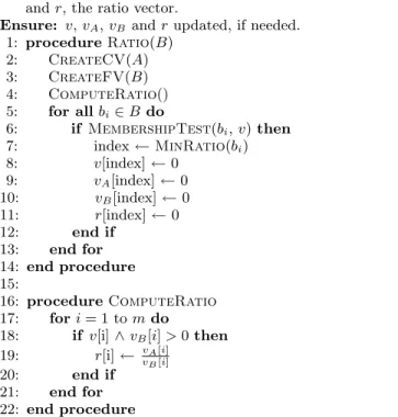
Finally, we propose a selective clearing mechanism called Ratio Selection. The idea is to combine Minimum FN
Se-Algorithm 3Maximum FP Selection
Require: v, the bit vector and vB, the counting vector.
Ensure: vand vBupdated, if needed.
1: procedure MaximumFP(B) 2: CreateFV(B) 3: for allbi∈ B do 4: if MembershipTest(bi, v) then 5: index ← MaxIndex(bi) 6: v[index] ← 0 7: vB[index] ← 0 8: end if 9: end for 10: end procedure 11: 12: procedure CreateFV(B) 13: for allbi∈ B do 14: forj= 1 to k do 15: vB[hj(bi)]++ 16: end for 17: end for 18: end procedure
lection and Maximum FP Selection into a single algorithm. Ratio Selection provides an approach in which we try to minimize the false negatives generated while maximizing the false positives removed. Ratio Selection therefore takes into account the risk of collision between hashed keys of elements belonging to A and hashed keys of elements belonging to B. It is achieved by maintaining a ratio vector, r, in which each position is the ratio between vA and vB. For each
troublesome key that was not previously cleared, we choose the index where the ratio is the minimum amongst the k ones. This index is given by the MinRatio function in Algo-rithm 4. Ratio Selection is defined in AlgoAlgo-rithm 4. This al-gorithm makes use of the CreateCV and CreateFV func-tions previously defined for Algorithms 2 and 3.
Details on the algorithmic and spatial complexity of these selective clearing algorithms are to be found in our technical report [6].
4.2
Evaluation
We conduct an experiment with a universe U of 2,000,000 elements (N = 2,000,000). These elements, for the sake of simplicity, are integers belonging to the range [0; 1,999,9999]. The subset A that we want to summarize in the Bloom filter contains 10,000 different elements (n = 10,000) randomly chosen from the universe U . Bloom’s paper [1] states that |U | must be much greater than |A|, without specifying a precise scale.
The bit vector v we use for simulations is 100,000 bits long (m = 100,000), ten times bigger than |A|. The RBF uses five different and independent hash functions (k = 5). Hashing is emulated with random numbers. We simulate randomness with the Mersenne Twister MT19937 pseudo-random number generator [7]. Using five hash functions and a bit vector ten times bigger than n is advised by Fan et al. [5]. This permits a good trade-off between membership query accuracy, i.e., a low false positive rate of 0.0094 when estimated with eqn. 5, memory usage and computation time. As mentioned earlier in this paper (see Sec. 2), the false positive rate may be decreased by increasing the bit vector size but it leads to a lower compression level.
Algorithm 4Ratio Selection
Require: v, the bit vector, vBand vA, the counting vectors
and r, the ratio vector.
Ensure: v, vA, vB and r updated, if needed.
1: procedure Ratio(B) 2: CreateCV(A) 3: CreateFV(B) 4: ComputeRatio() 5: for allbi∈ B do 6: if MembershipTest(bi, v) then 7: index ← MinRatio(bi) 8: v[index] ← 0 9: vA[index] ← 0 10: vB[index] ← 0 11: r[index] ← 0 12: end if 13: end for 14: end procedure 15: 16: procedure ComputeRatio 17: fori= 1 to m do
18: if v[i] ∧ vB[i] > 0 then
19: r[i] ← vA[i]
vB[i]
20: end if
21: end for 22: end procedure
For our experiment, we define the ratio of troublesome keys compared to the entire set of false positives as
β = |B| |FP|
(17) We consider the following values of β: 1%, 2%, 5%, 10%, 25%, 50%, 75% and 100%. When β = 100%, it means that B= FPand we want to remove all the false positives.
Each data point in the plots represents the mean value over fifteen runs of the experiment, each run using a new A, FP, B, and RBF. We determine 95% confidence intervals
for the mean based on the Student t distribution.
We perform the experiment as follows: we first create the universe U and randomly affect 10,000 of its elements to A. We next build FPby applying the following scheme. Rather
than using eqn. 5 to compute the false positive rate and then creating FPby randomly affecting positions in v for the false
positive elements, we prefer to experimentally compute the false positives. We query the RBF with a membership test for each element belonging to U − A. False positives are the elements that belong to the Bloom filter but not to A. We keep track of them in a set called FP. This process seems
to us more realistic because we evaluate the real quantity of false positive elements in our data set. B is then constructed by randomly selecting a certain quantity of elements in FP,
the quantity corresponding to the desired cardinality of B. We next remove all troublesome keys from B by using one of the selective clearing algorithms, as explained in Sec. 4.1. We then build F′
N, the false negative set, by testing all
el-ements in A and adding to F′
N all elements that no longer
belong to A. We also determine F′
P, the false positive set
after removing the set of troublesome keys B.
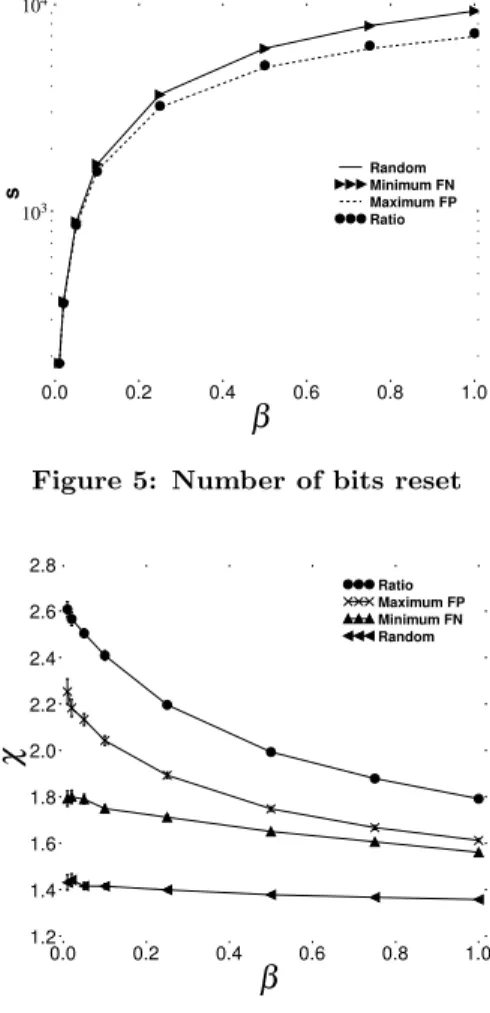
Fig. 5 compares the four algorithms in terms of the num-ber s of reset bits required to remove troublesome keys in B. The horizontal axis gives β and the vertical axis, in log
Figure 5: Number of bits reset
Figure 6: Effect onχ
scale, gives s. The confidence intervals are plotted but they are too tight to appear clearly.
We see that Random Selection and Minimum FN Selec-tion need to work more, in terms of number of bits to reset, when β grows, compared to Maximum FP Selection and Ra-tio SelecRa-tion. In addiRa-tion, we note that the RaRa-tio SelecRa-tion algorithm needs to reset somewhat more bits than Maxi-mum FP Selection (the difference is too tight to be clearly visible on the plots).
Fig. 6 evaluates the performance of the four algorithms. It plots β on the horizontal axis and χ on the vertical axis. Again, the confidence intervals are plotted but they are gen-erally too tight to be visible.
We first note that, whatever the algorithm considered, the χratio is always above 1, meaning that the advantages of removing false positives overcome the drawbacks of gener-ating false negatives, if these errors are considered equally grave. Thus, as expected, performing selective clearing pro-vides better results than randomized bit clearing. Ratio Se-lection does best, followed by Maximum FP, Minimum FN, and Ratio Selection.
The χ ratio for Random Selection does not vary much with βcompared to the three other algorithms. For instance, the χratio for Ratio Selection is decreased by 31.3% between β=1% and β=100%.
To summarize, one can say that, when using RBF, one can reliably get a χ above 1.4, even when using a simple selective
clearing algorithm, such as Random Selection. Applying a more efficient algorithm, such as Ratio Selection, allows one to get a χ above 1.8. Such χ values mean that the proportion of false positives removed is higher than the proportion of false negatives generated.
In this section, we provided and evaluated four simple selective algorithms. We showed that two algorithms, Max-imum FP Selection and Ratio Selection, are more efficient in terms of number of bits to clear in the filter. Among these two algorithms, we saw that Ratio Selection provides better results, in terms of the χ ratio.
5.
CASE STUDY
Retouched Bloom filters can be applied across a wide range of applications that would otherwise use Bloom fil-ters. For RBFs to be suitable for an application, two criteria must be satisfied. First, the application must be capable of identifying instances of false positives. Second, the applica-tion must accept the generaapplica-tion of false negatives, and in particular, the marginal benefit of removing the false posi-tives must exceed the marginal cost of introducing the false negatives.
This section describes the application that motivated our introduction of RBFs: a network measurement system that traces routes, and must communicate information concern-ing IP addresses at which to stop tracconcern-ing. Sec. 5.1 evaluates the impact of using RBFs in this application.
Maps of the internet at the IP level are constructed by tracing routes from measurement points distributed through-out the internet. The skitter system [8], which has provided data for many network topology papers, launches probes from 24 monitors towards almost a million destinations. However, a more accurate picture can potentially be built by using a larger number of vantage points. Dimes [9] heralds a new generation of large-scale systems, counting, at present 8,700 agents distributed over five continents. As Donnet et al. [10] (including authors on the present paper) have pointed out, one of the dangers posed by a large number of monitors probing towards a common set of destinations is that the traffic may easily be mistaken for a distributed denial of service (DDoS) attack.
One way to avoid such a risk would be to avoid hitting destinations. This can be done through smart route tracing algorithms, such as Donnet et al.’s Doubletree [10]. With Doubletree, monitors communicate amongst themselves re-garding routes that they have already traced, in order to avoid duplicating work. Since one monitor will stop trac-ing a route when it reaches a point that another monitor has already traced, it will not continue through to hit the destination.
Doubletree considerably reduces, but does not entirely eliminate, DDoS risk. Some monitors will continue to hit destinations, and will do so repeatedly. One way to further scale back the impact on destinations would be to introduce an additional stopping rule that requires any monitor to stop tracing when it reaches a node that is one hop before that destination. We call such a node the penultimate node, and we call the set of penultimate nodes the red stop set (RSS). A monitor is typically not blocked by its own first-hop node, as it will normally see a different IP address from the addresses that appear as penultimate nodes on incoming traces. This is because a router has multiple interfaces, and the IP address that is revealed is supposed to be the one that
sends the probe reply. The application that we study in this paper conducts standard route traces with an RSS. We do not use Doubletree, so as to avoid having to disentangle the effects of using two different stopping rules at the same time. How does one build the red stop set? The penultimate nodes cannot be determined a priori. However, the RSS can be constructed during a learning round in which each monitor performs a full set of standard traceroutes, i.e., until hitting a destination. Monitors then share their RSSes. For simplicity, we consider that they all send their RSSes to a central server, which combines them to form a global RSS, that is then redispatched to the monitors. The monitors then apply the global RSS in a stopping rule over multiple rounds of probing.
Destinations are only hit during the learning round and as a result of errors in the probing rounds. DDoS risk di-minishes with an increase in the ratio of probing rounds to learning rounds, and with a decrease in errors during the probing rounds. DDoS risk would be further reduced if we apply Doubletree in the learning round, as the number of probes that reach destinations during the learning round would then scale less then linearly in the number of mon-itors. However, our focus here is on the probing rounds, which use the global RSS, and not on improving the effi-ciency of the learning round, which generates the RSS, and for which we already have known techniques.
The communication cost for sharing the RSS among mon-itors is linear in the number of monmon-itors and in the size of the RSS representation. It is this latter size that we would like to reduce by a constant compression factor. If the RSS is implemented as a list of 32-bit vectors, skitter’s million destinations would consume 4 MB. We therefore propose encoding the RSS information in Bloom filters. Note that the central server can combine similarly constructed Bloom filters from multiple monitors, through bitwise logical or operations, to form the filter that encodes the global RSS.
The cost of using Bloom filters is that the application will encounter false positives. A false positive, in our case study, corresponds to an early stop in the probing, i.e., before the penultimate node. We call such an error stopping short, and it means that part of the path that should have been dis-covered will go unexplored. Stopping short can also arise through network dynamics, when additional nodes are in-troduced, by routing changes or IP address reassignment, between the previously penultimate node and the destina-tion. In contrast, a trace that stops at a penultimate node is deemed a success. A trace that hits a destination is called a collision. Collisions might occur because of a false negative for the penultimate node, or simply because routing dynam-ics have introduced a new path to the destination, and the penultimate node on that path was previously unknown.
As we show in Sec. 5.1, the cost of stopping short is far from negligible. If a node that has a high betweenness cen-trality (Dall’Asta et al. [11] point out the importance of this parameter for topology exploration) generates a false positive, then the topology information loss might be high. Consequently, our idea is to encode the RSS in an RBF.
As described in the Introduction, there are two criteria for being able to profitably employ RBFs, and they are both met by this application. First, false positives can be iden-tified and removed. Once the topology has been revealed, each node can be tested against the Bloom filter, and those that register positive but are not penultimate nodes are false
positives. The application has the possibility of removing the most troublesome false positives by using one of the se-lective algorithms discussed in Sec. 4. Second, a low rate of false negatives is acceptable and the marginal benefit of removing the most troublesome false positives exceeds the marginal cost of introducing those false negatives. Our aim is not to eliminate collisions; if they are considerably re-duced, the DDoS risk has been diminished and the RSS application can be deemed a success. On the other hand, systematically stopping short at central nodes can severely restrict topology exploration, and so we are willing to ac-cept a low rate of random collisions in order to trace more effectively. These trade-offs are explored in Sec. 5.1.
Table 1 summarizes the positive and negative aspects of each RSS implementation we propose. Positive aspects are a success, stopping at the majority of penultimate nodes, topology information discovered, the eventual compression ratio of the implementation, and a low number of collisions with destinations. Negative aspects of an implementation can be the topology information missed due to stopping short, the load on the network when exchanging the RSS and the risk of hitting destinations too many times. Sec. 5.1 examines the positive and negative aspects of each imple-mentation.
5.1
Evaluation
In this section, we evaluate the use of RBFs in a tracerout-ing system based on an RSS. We first present our method-ology and then, discuss our results.
Our study is based on skitter data [8] from January 2006. This data set was generated by 24 monitors located in the United States of America, Canada, the United Kingdom, France, Sweden, the Netherlands, Japan, and New Zealand. The monitors share a common destination set of 971,080 IPv4 addresses. Each monitor cycles through the destina-tion set at its own rate, taking typically three days to com-plete a cycle.
For the purpose of our study, in order to reduce computing time to a manageable level, we work from a limited set of 10 skitter monitors, all the monitors sharing a list of 10,000 destinations, randomly chosen from the original set. In our data set, the RSS contains 8,006 different IPv4 addresses.
We compare the following three RSS implementations: list, Bloom filter and RBF. The list would not return any er-rors if the network were static, however, as discussed above, network dynamics lead to a certain error rate of both colli-sions and instances of stopping short. For the RBF imple-mentation, we consider β values (see eqn. 17) of 1%, 5%, 10% and 25%. We employ the Ratio Selection algorithm, as defined in Sec. 4.1. For the Bloom filter and RBF implemen-tations, the hashing is emulated with random numbers. We simulate randomness with the Mersenne Twister MT19937 pseudo-random number generator [7].
To obtain our results, we simulate one learning round on a first cycle of traceroutes from each monitor, to generate the RSS. We then simulate one probing round, using a sec-ond cycle of traceroutes. In this simulation, we replay the traceroutes, but apply the stopping rule based on the RSS, noting instances of stopping short, successes, and collisions. Fig. 7 compares the success rate, i.e., stopping at a penul-timate node, of the three RSS implementations. The hori-zontal axis gives different filters size, from 10,000 to 100,000, with an increment of 10,000. Below the horizontal axis sits
Implementation Positive Negative
Success Topo. discovery Compression No Collision Topo. missed Load Collision
List X X X X
Bloom filter X X X
RBF X X X X
Table 1: Positive and negative aspects of each RSS implementation
Figure 7: Success rate
another axis that indicates the compression ratio of the fil-ter, compared to the list implementation of the RSS. The vertical axis gives the success rate. A value of 0 would mean that using a particular implementation precludes stopping at the penultimate node. On the other hand, a value of 1 means that the implementation succeeds in stopping each time at the penultimate node.
Looking first at the list implementation (the horizontal line), we see that the list implementation success rate is not 1 but, rather, 0.7812. As explained in Sec. 5.1, this can be explained by the network dynamics such as routing changes and dynamic IP address allocation.
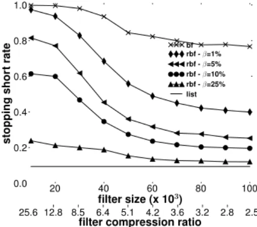
With regards to the Bloom filter implementation, we see that the results are poor. The maximum success rate, 0.2446, is obtained when the filter size is 100,000 (a compression ra-tio of 2.5 compared to the list). Such poor results can be explained by the troublesomeness of false positives. Fig. 8 shows, in log-log scale, the troublesomeness distribution of false positives. The horizontal axis gives the troublesome-ness degree, defined as the number of traceroutes that stop short for a given key. The maximum value is 104, i.e., the number of traceroutes performed by a monitor. The verti-cal axis gives the number of false positive elements having a specific troublesomeness degree. The most troublesome keys are indicated by an arrow towards the lower right of the graph: nine false positives are, each one, encountered 10,000 times.
Looking now, in Fig. 7, at the success rate of the RBF, we see that the maximum success rate is reached when β = 0.25. We also note a significant increase in the success rate for RBF sizes from 10,000 to 60,000. After that point, except for β = 1%, the increase is less marked and the suc-cess rate converges to the maximum, 0.7564. When β = 0.25, for compression ratios of 4.2 and lower, the success rate approaches that of the list implementation. Even for compression ratios as high as 25.6, it is possible to have a success rate over a quarter of that offered by the list
imple-Figure 8: Troublesomeness distribution
Figure 9: Stopping short rate
mentation.
Fig. 9 gives the stopping short rate of the three RSS im-plementations. A value of 0 means that the RSS implemen-tation does not generate any instances of stopping short. On the other hand, a value of 1 means that every stop was short.
Looking first at the list implementation, one can see that the stopping short rate is 0.0936. Again, network dynamics imply that some nodes that were considered as penultimate nodes during the learning phase are no longer located one hop before a destination.
Regarding the Bloom filter implementation, one can see that the stopping short rate is significant. Between 0.9981 (filter size of 103) and 0.7668 (filter size of 104). The cost
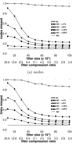
of these high levels of stopping short can be evaluated in terms of topology information missed. Fig. 10 compares the RBF and the Bloom filter implementation in terms of nodes (Fig. 10(a)) and links (Fig. 10(b)) missed due to stopping short. A value of 1 means that the filter implementation
(a) nodes
(b) links
Figure 10: Topology information missed
missed all nodes and links when compared to the list im-plementation. On the other hand, a value of 0 mean that there is no loss, and all nodes and links discovered by the list implementation are discovered by the filter implementa-tion. One can see that the loss, when using a Bloom filter, is above 80% for filter sizes below 70,000.
Implementing the RSS as an RBF allows one to decrease the stopping short rate. When removing 25% of the most troublesome false positives, one is able to reduce the stop-ping short between 76.17% (filter size of 103) and 84,35%
(filter size of 104). Fig. 9 shows the advantage of using an RBF instead of a Bloom filter. Fig. 10 shows this advantage in terms of topology information. We miss a much smaller quantity of nodes and links with RBFs than Bloom filters and we are able to nearly reach the same level of coverage as with the list implementation.
Fig. 11 shows the cost in terms of collisions. Collisions will arise under Bloom filter and list implementations only due to network dynamics. Collisions can be reduced under all RSS implementations due to a high rate of stopping short (though this is, of course, not desired). The effect of stop-ping short is most pronounced for RBFs when β is low, as shown by the curve β = 0.01. One startling revelation of this figure is that even for fairly high values of β, such as β= 0.10, the effect of stopping short keeps the RBF collision cost lower than the collision cost for the list implementation, over a wide range of compression ratios. Even at β = 0.25,
Figure 11: Collision cost
Figure 12: Metrics for an RBF with m=60,000
the RBF collision cost is only slightly higher.
Fig. 12 compares the success, stopping short, and collision rates for the RBF implementation with a fixed filter size of 60,000 bits. We vary β from 0.01 to 1 with an increment of 0.01. We see that the success rate increases with β until reaching a peak at 0.642 (β = 0.24), after which it decreases until the minimum success rate, 0.4575, is reached at β = 1. As expected, the stopping short rate decreases with β, varying from 0.6842 (β = 0) to 0 (β = 1). On the other hand, the collision rate increases with β, varying from 0.0081 (β = 0) to 0.5387 (β = 1).
The shaded area in Fig. 12 delimits a range of β values for which success rates are highest, and collision rates are rel-atively low. This implementation gives a compression ratio of 4.2 compared to the list implementation. The range of βvalues (between 0.1 and 0.3) gives a success rate between 0.7015 and 0.7218 while the list provides a success rate of 0.7812. The collision rate is between 0.1073 and 0.1987, meaning that in less than 20% of the cases a probe will hit a destination. On the other hand, a probe hits a destination in 12.51% of the cases with the list implementation. Finally, the stopping short rate is between 0.2355 and 0.1168 while the list implementation gives a stopping short rate of 0.0936. In closing, we emphasize that the construction of B and the choice of β in this case study are application specific. We do not provide guidelines for a universal means of determin-ing which false positives should be considered particularly
troublesome, and thus subject to removal, across all applica-tions. However, it should be possible for other applications to measure, in a similar manner as was done here, the po-tential benefits of introducing RBFs.
6.
RELATED WORK
Bloom’s original paper [1] describes the use of his data structure for a hyphenation application. As described in Broder and Mitzenmacher’s survey [3], early applications were for dictionaries and databases. In recent years, as the survey describes, there has been considerable interest in the use of Bloom filters in networking applications. Authors of the present paper have earlier described the use of Bloom filters for a network measurement application [12]. Other examples abound.
The Bloom filter variant that is closest in spirit to the RBF is Hardy’s anti-Bloom filter [13], as it allows explicit overriding of false positives. An anti-Bloom filter is a smaller filter that accompanies a standard Bloom filter. When que-ried, the combination generates a negative result if either the main filter does not recognize a key or the anti-filter does.
Compared to the anti-Bloom filter, an advantage of the RBF is that it requires no additional space beyond that which is used by a standard Bloom filter. However, a thor-ough analysis of the comparative merits would be of inter-est. This would require an examination of how to best size an anti-filter, and a study of the trade-offs between false positives suppressed and false negatives generated by the anti-filter.
Another variant that is close in spirit to the RBF is Fan et al.’s counting Bloom filter (CBF) [5], as it allows explicit removal of elements from the filter. The CBF effectively replaces each cell of a Bloom filter’s bit vector with a multi-bit counter, so that instead of storing a simple 0 or a 1, the cell stores a count. This additional space allows CBFs to not only encode set membership information, as standard Bloom filters do, but to also permit dynamic additions and deletions of that information. One consequence of this new flexibility is that there is a chance of generating false negatives. They can arise if the counters overflow. Fan et al. suggest that the counters be sized to keep the probability of false negatives to such a low threshold that they are not a factor for the application (four bits being adequate in their case).
RBFs differ from CBFs in that they are designed to re-move false positives, rather than elements that are truly encoded in the filter. Whereas the CBF’s counting tech-nique could conceivably be used to remove false positives, by decrementing their counts, we do not believe that this would be a fruitful approach. Consider a CBF with the same spatial complexity as an RBF, that is, with a one bit counter. Decrementing the count for a false positive in a CBF would mean resetting as many as k bits, one for each hash function. The resetting operation in an RBF involves only one of these bits, so it will necessarily generate fewer false negatives.
There are few studies of the possibility of trading off false positives against false negatives in variants of Bloom fil-ters. An exception is Laufer et al.’s careful analysis [14] of the trade-offs for their generalized Bloom filter (GBF) [15]. With the GBF, one moves beyond the notion that elements must be encoded with 1s, and that 0s represent the absence of information. A GBF starts out as a random vector of
both 1s and 0s, and information is encoded by setting cho-sen bits to either 0 or 1. As a result, the GBF is a more general binary classifier than the standard Bloom filter, with as one consequence that it can produce either false positives or false negatives.
A GBF employs two sets of hash functions, g1, . . . , gk0and h1, . . . , hk1to set and reset bits. To add an element x to the GBF, the bits corresponding to the positions g1(x), . . . , gk0(x) are set to 0 and the bits corresponding to h1(x), . . . , hk1(x) are set to 1. In the case of a collision between two hash values gi(x) and hj(x), the bit is set to 0. The
member-ship of an element y is verified by checking if all bits at g1(y), . . . , gk0(y) are set to 0 and all bits at h1(y), . . . , hk1(y) are set to 1. If at least one bit is inverted, y does not belong to the GBF with a high probability. A false negative arises when at least one bit of g1(y), . . . , gk0(y) is set to 1 or one bit of h1(y), . . . , hk1(y) is set to 0 by another element inserted afterwards. The rates of false positives and false negatives in a GBF can be traded off by varying the numbers of hash functions, k0and k1, as well as other parameters such as the
size of the filter.
RBFs differ from GBFs in that they allow the explicit re-moval of selected false positives. RBFs also do so in a way that allows the overall error rate, expressed as a combina-tion of false positives and false negatives, to be lowered as compared to a standard Bloom filter of the same size. We note that the techniques used to remove false positives from standard Bloom filters could be extended to remove false positives from GBFs. For a false positive key, x, either one would set one of the bits g1(x), . . . , gk0(x) to 1 or one of the bits h1(x), . . . , hk1(x) to 0.
Bonomi et al. also provide a Bloom filter variant in which it is possible to trade off false positives and false negatives. Their d-left counting Bloom filter (dlCBF) [4, 16], has as its principal advantage a greater space efficiency than the CBF. Like the CBF, it can produce false negatives. It can also produce another type of error called “don’t know”. Bonomi et al. describe experiments that measure the rates for the different kinds of errors.
RBFs differ from dlCBFs in the same way as they differ from standard CBFs: they are designed to remove false posi-tives rather than elements that have been explicitly encoded into the vector, and they do so by resetting one single bit rather than decrementing a series of bits.
7.
CONCLUSION
The Bloom filter is a lossy summary technique that has attracted considerable attention from the networking re-search community for the bandwidth efficiencies it provides in transmitting set membership information between net-worked hosts.
In this paper, we introduced the retouched Bloom filter (RBF), an extension that makes Bloom filters more flexible by permitting selected false positives to be removed at the expense of introducing some random false negatives. The key idea is to remove each false positive by resetting a care-fully chosen bit in the bit vector that makes up the filter.
We analytically demonstrated that the trade-off between false positives and false negatives is at worst neutral, on average, when randomly resetting bits in the bit vector, whether these bits correspond to false positives or not. We also proposed four algorithms for efficiently deleting false positives. We evaluated these algorithms through
simula-tion and showed that RBFs created in this manner will in-crease the false negative rate by less than the amount by which the false positive rate is decreased.
In this paper, we described a network measurement appli-cation for which RBFs can profitably be used. In this case study, traceroute monitors, rather than stopping probing at a destination, terminate their measurement at the penulti-mate node. The monitors share information on the set of penultimate nodes, the red stop set (RSS). We compared three different implementations for representing the RSS in-formation: list, Bloom filter, and RBF. Using filters reduces the bandwidth requirements, but the false positives can sig-nificantly impact the amount of topology information that the system gleans. We demonstrated that using an RBF, in which the most troublesome false positives are removed, will increase the coverage of a filter implementation. While the rate of collisions with destinations will increase, it can still be lower than for the list implementation.
In future work, we hope to demonstrate techniques to ap-ply the RBF concept earlier in the construction of the filter. At present, we allow the Bloom filter to be built, and then remove the most troublesome false positives. It should be possible to avoid recording some of these false positives in the filter to begin with.
Acknowledgements
Mr. Donnet’s work was partially supported by a SATIN grant provided by the E-NEXT doctoral school, by an in-ternship at Caida, and by the European Commission-funded OneLab project. Mark Crovella introduced us to Bloom fil-ters and encouraged our work. Rafael P. Laufer suggested useful references regarding Bloom filter variants. Otto Car-los M. B. Duarte helped us clarify the relationship of RBFs to such variants. We thank k claffy and her team at Caida for allowing us to use the skitter data.
8.
REFERENCES
[1] B. H. Bloom, “Space/time trade-offs in hash coding with allowable errors,” Communications of the ACM, vol. 13, no. 7, pp. 422–426, 1970.
[2] M. Mitzenmacher, “Compressed Bloom filters,” IEEE/ACM Trans. on Networking, vol. 10, no. 5, 2002.
[3] A. Broder and M. Mitzenmacher, “Network applications of Bloom filters: A survey,” Internet Mathematics, vol. 1, no. 4, 2002.
[4] F. Bonomi, M. Mitzenmacher, R. Panigraphy, S. Singh, and G. Varghese, “Beyond Bloom filters: From approximate membership checks to approximate state machines,” in Proc. ACM SIGCOMM, Sept. 2006.
[5] L. Fan, P. Cao, J. Almeida, and A. Z. Broder, “Summary cache: a scalable wide-area Web cache sharing protocol,” IEEE/ACM Trans. on Networking, vol. 8, no. 3, pp. 281–293, 2000.
[6] B. Donnet, B. Baynat, and T. Friedman, “Retouched Bloom filters: Allowing networked applications to trade off selected false positives against false negatives,” arXiv, cs.NI 0607038, Jul. 2006.
[7] M. Matsumoto and T. Nishimura, “Mersenne Twister: A 623-dimensionally equidistributed uniform
pseudorandom number generator,” ACM Trans. on Modeling and Computer Simulation, vol. 8, no. 1, pp. 3–30, Jan. 1998.
[8] B. Huffaker, D. Plummer, D. Moore, and k. claffy, “Topology discovery by active probing,” in Proc. SAINT, Jan. 2002.
[9] Y. Shavitt and E. Shir, “DIMES: Let the internet measure itself,” ACM SIGCOMM Computer Communication Review, vol. 35, no. 5, 2005.
[10] B. Donnet, P. Raoult, T. Friedman, and M. Crovella, “Efficient algorithms for large-scale topology
discovery,” in Proc. ACM SIGMETRICS, 2005. [11] L. Dall’Asta, I. Alvarez-Hamelin, A. Barrat,
A. V´asquez, and A. Vespignani, “A statistical approach to the traceroute-like exploration of networks: Theory and simulations,” in Proc. CAAN Workshop, Aug. 2004.
[12] B. Donnet, T. Friedman, and M. Crovella, “Improved algorithms for network topology discovery,” in Proc. PAM Workshop, 2005.
[13] N. Hardy, “A little Bloom filter theory (and a bag of filter tricks),” 1999, see
http://www.cap-lore.com/code/BloomTheory.html. [14] R. P. Laufer, P. B. Velloso, and O. C. M. B. Duarte,
“Generalized Bloom filters,” Electrical Engineering Program, COPPE/UFRJ, Tech. Rep., 2005. [15] R. P. Laufer, P. B. Velloso, D. de O. Cunha, I. M.
Moraes, M. D. D. Bicudo, and O. C. M. B. Duarte, “A new IP traceback system against distributed denial-of-service attacks,” in Proc. 12th ICT, 2005. [16] F. Bonomi, M. Mitzenmacher, R. Panigrahy, S. Singh,
and G. Varghese, “An improved construction for counting Bloom filters,” in Proc. ESA, Sept. 2006.