A study of skeleta in non-Archimedean geometry

(1)

HAL Id: tel-01206486

https://tel.archives-ouvertes.fr/tel-01206486

Submitted on 29 Sep 2015

HAL is a multi-disciplinary open access

archive for the deposit and dissemination of

sci-entific research documents, whether they are

pub-lished or not. The documents may come from

teaching and research institutions in France or

L’archive ouverte pluridisciplinaire HAL, est

destinée au dépôt et à la diffusion de documents

scientifiques de niveau recherche, publiés ou non,

émanant des établissements d’enseignement et de

recherche français ou étrangers, des laboratoires

A study of skeleta in non-Archimedean geometry

John Welliaveetil

To cite this version:

John Welliaveetil. A study of skeleta in non-Archimedean geometry. General Mathematics [math.GM].

Université Pierre et Marie Curie - Paris VI, 2015. English. �NNT : 2015PA066162�. �tel-01206486�

(2)

(3)

Abstract

This thesis is a reflection of the interaction between Berkovich geometry and model theory. Using the results of Hrushovski and Loeser [HL], we show that several interesting topological phenomena that concern the analytifications of varieties are governed by certain finite simplicial complexes embedded in them. Our work consists of the following two sets of results.

Let k be an algebraically closed non-Archimedean non trivially real valued field which is complete with respect to its valuation.

1. Let φ : C0 → C be a finite morphism between smooth projective irre-ducible k-curves. The morphism φ induces a morphism φan_{: C}0an _{→ C}an

between the Berkovich analytifications of the curves. We construct a pair of deformation retractions of C0an _{and C}an _{which are compatible with}

the morphism φan_{and whose images Υ}

C0an, Υ_Can are closed subspaces of

C0an_{, C}an _{that are homeomorphic to finite metric graphs. We refer to}

such closed subspaces as skeleta. In addition, the subspaces ΥC0an and

ΥCan are such that their complements in their respective analytifications

decompose into the disjoint union of isomorphic copies of Berkovich open balls. The skeleta can be seen as the union of vertices and edges, thus allowing us to define their genus. The genus of a skeleton in a curve C is in fact an invariant of the curve which we call gan_{(C). The pair of}

com-patible deformation retractions forces the morphism φan _{to restrict to a}

map ΥC0an → Υ_Can. We study how the genus of Υ_C0an can be calculated

using the morphism φan

|ΥC0an and invariants defined on ΥC an.

2. Let φ be a finite endomorphism of P1

k. Given a closed point x ∈ P1k, we are

interested in the radius f (x) of the largest Berkovich open ball centered at x over which the morphism φan_{is a topological fibration. Interestingly,}

the function f : P1

k(k) → R≥0admits a strong tameness property in that it

is controlled by a non-empty finite graph contained in P1,an_k . We show that this result can be generalized to the case of finite morphisms φ : V0_{→ V}

(4)

Abstract

Cette thèse s’appuie sur et reflète l’interaction entre la théorie des modèles et la géométrie de Berkovich. En utilisant les méthodes de Hrushovski et Loeser [HL], nous montrerons que plusieurs phénomènes topologiques concernant des analytifications de variétés sont contrôlés par certains complexes simpliciaux contenus dans les analytifications. Ce travail comporte les résultats suivants.

Soit k un corps algébriquement clos et complet pour une valuation non-archimédienne non-triviale à valeurs réelles.

1. Soit φ : C0 → C un morphisme fini entre deux courbes projectives, lisses et irr´eductibles. Le morphisme φ induit un morphisme φan_{: C}0an_{→ C}an

entre les deux analytifications. Nous construisons une paire de rétractions par déformations qui sont compatible pour le morphisme φan. Les images des déformations ΥC0an, Υ_Can sont des sous-espaces fermés de C0an and

Can _{et hom´eomorphes `a des graphes finis. Ce type de sous-espace est}

appel´e squelette. En outre, les espaces analytiques C0an_{r Υ}

C0an et Canr

ΥCan se d´ecomposent en une union disjointe de copies de disques unit´es

de Berkovich. Un squelette Υ ⊂ Can_{peut-être décomposé en un ensemble}

des sommets et un ensemble d’arêtes et on peut définir son genre g(Υ). Nous montrons que g(Υ) est un invariant bien défini de la courbe C. On appelle cet invariant gan_{(C). Le morphisme φ}an _{induira un morphisme}

ΥC0an → Υ_Can entre les deux squelettes. Nous montrons que le genre du

squelette ΥC0an peut être calculé en utilisant certains invariants associés

aux points de ΥCan.

2. Soit φ un endomorphisme fini de P1

k. Soit x ∈ P1k(k) et f (x) le rayon de la

plus grande boule de Berkovich de centre x, sur laquelle le morphisme φan

est une fibration topologique. Nous voyons que la fonction f : P1 k(k) →

R≥0 est contrˆol´ee par un graphe fini et non-vide contenu dans P1,ank . Nous

montrons que ce résultat peut être généralisé au cas d’un morphisme fini φ : V0_{→ V entre deux variétés intégrales, projectives avec V normale.}

(5)

Acknowledgements

This thesis would never have been possible without the constant support and guidance of my advisor - Fran¸cois Loeser. His patience and generosity have made possible my research to date and for this I shall always be grateful. Over the course of my PhD, our weekly meetings have illuminated several aspects of mathematics that I could never have learnt from another source.

I must thank Jérôme Pôineau for his time and diligent reading of the first drafts of the results presented below. His efforts greatly improved the presen-tation of the two articles that I have written and furthermore brought to my attention subtleties I had previously overlooked. Professeur Pôineau has always been a source of encouragement, quick to respond to a technical question and open to discussion. I am grateful that he agreed to act as a rapporteur.

I am honoured that Professor Annette Werner agreed to act as my second rapporteur and I greatly appreciated her opinion of the results presented below. I am grateful as well to the other members of the jury - Jean-Fran¸cois Dat, Bertrand Remy and Martin Hils who have taken time out of their schedules to attend the soutenance.

These years in Paris during which I made my way fumbling, through the arcane, esoteric world of pure mathematics were always dotted by happy coin-cidence - itinerant post-docs - Yimu, Michel and Ethan setting up shop down the corridor or a long list of fellow PhD students in neighbouring offices with whom I learnt to speak in french and in whose company, the taste of cold beer after a days work never tasted as sweet. My deepest gratitude to Arthur with whom I shared an office for more than a year and from whom I learnt a great deal of interesting mathematics. I must also mention Hsueh-Yung and Valentin who have always been available for coffee or the quick discussion of a problem I found myself stuck on. And then there is Ildar Gaisin whose presence greatly al-leviated the sobering effects that often accompanies the writing of a PhD thesis. It is the afternoon breaks and the relaxed discussions of mathematics amidst our frequent coffees that sustained me through several difficult passages during the last two years. Despite long since having fled these shores, Giovanni Rosso continues to offer his services at a moments notice and though his physical pres-ence and famous risotto are things of the past, his friendship and support are forever present.

I would be remiss if I did not mention my friends who did not do mathematics but deeply enriched my life in Paris. My work would have greatly suffered without the many relaxed evenings, free dinners and wine by the seine I owe to Praavita, Jyotsna, Asha, Lara, Florence, Marine, Raghav, William and Nithya. I must thank Sarah for her warmth and patience. The prospect of an isolated three years loomed large when I first came to France completely ignorant of the language. It was my good fortune to have met Lara a week after first coming to France and the wealth of happy memories that the ensuing years brought with them. Although I had written and submitted my thesis before I met Eliza, her presence has brightened the mundane and simplified the ups and downs of doing research.

Lastly, I must thank my extended family who supported my work and for their generosity, love and kindness. My mother’s knowledge of mathematics is limited but her guidance has always held me in good stead and it is to her that I dedicate my thesis.

(6)

Introduction

Non-Archimedean fields were discovered at the turn of the twentieth century when K. Hensel defined the field of p-adic numbers Qp. Ever since, there have

been attempts, each with its merits, to develop a theory of geometry over such fields analogous to the theory of complex geometry. However, it was only in the early nineties that Vladmir Berkovich developed a theory of non-Archimedean geometry which provided analytic spaces endowed with reasonable topologi-cal properties. In the framework of this geometry, a variety defined over a non-Archimedean field defines an associated Berkovich analytic space called its analytification. Even though such varieties when endowed with the topology induced by the valuation of the ground field are totally disconnected, their an-alytifications are Hausdorff, locally compact and have a finite number of path connected components. It is hence natural to investigate the homotopy type of the analytification of such algebraic varieties.

In 2010, Hrushovski and Loeser using techniques from Model theory studied the homotopy type of the analytification of an algebraic variety defined over a non trivially valued non-Archimedean real valued field. They showed that these homotopy types are determined completely by finite simplicial complexes embedded in the analytification by constructing deformation retractions of the analytifications onto such complexes. In [HL], Hrushovski and Loeser define a model theoretic analogue of the Berkovich analytification of a variety. One of the advantages of this viewpoint is that it provides a framework within which we can discuss model theoretic notions such as definability and employ powerful methods such as compactness. This thesis is a reflection of this interaction between Berkovich geometry and model theory. We show that several interesting topological phenomena that concern the analytifications of varieties are governed by certain finite simplicial complexes embedded in them.

1.1 A Riemann-Hurwitz formula for the

ana-lytic genus

Let k be an algebraically closed, complete non-Archimedean non trivially real valued field. Let C be a k-curve. By k-curve, we mean a one dimensional connected reduced separated scheme of finite type over the field k. It is well

(9)

known that there exists a deformation retraction of Can_{onto a closed subspace}

Υ which is homeomorphic to a finite metric graph [[B], Chapter 4], [[HL], Section 7]. We call such subspaces skeleta. The skeleton Υ can be decomposed into a set of vertices V (Υ) and a set of edges E(Υ). We define the genus of the skeleton Υ as follows.

g(Υ) = 1 − V (Υ) + E(Υ).

In Proposition 7.1.24, we show that g(Υ) is a well defined invariant of the curve and does not depend on the retract Υ. Let gan(C) := g(Υ) for any such Υ. We study how gan _{varies for a finite morphism using a compatible pair of}

deformation retractions.

Let C0_{, C be smooth projective irreducible k-curves and φ : C}0 _{→ C be a}

finite morphism. The morphism φ induces a morphism between the respective analytifications which we denote φan_{. Hence we have}

φan_{: C}0an_{→ C}an_.

In Theorem 7.2.1, we prove that there exists a pair of compatible deformation retractions. The exact statement is as follows.

Theorem 7.2.1 Let C and C0 _{be smooth projective irreducible k-curves and}

φ : C0 _{→ C be a finite morphism. There exists a pair of deformation retractions}

ψ : [0, 1] × Can→ Can

and

ψ0: [0, 1] × C0an→ C0an with the following properties.

1. The images ΥC0an := ψ0(1, C0an) and Υ_Can := ψ(1, Can) are closed

sub-spaces of C0an_{and C}an_{respectively, each with the structure of a connected,}

finite metric graph. Furthermore, we have that ΥC0an = (φan)−1(Υ_Can).

2. The analytic spaces C0an _{r Υ}

C0an and Canr Υ_Can decompose into the

disjoint union of isomorphic copies of Berkovich open disks i.e. there exist weak semistable vertex sets (cf. Definition 7.1.18) A ⊂ Can _and

A0 ⊂ C0an _{such that Υ}

Can= Σ(Can, A) and Υ_C0an = Σ(C0an, A0).

3. The deformation retractions ψ and ψ0 _{are compatible i.e. the following}

diagram is commutative. [0, 1] × Can _Can [0, 1] × C0an _C0an ? ? -ψ ψ0 id × φan _φan_.

(10)

In Sections 7.3 and 7.4, we study how gan_(C0_{) and g}an_{(C) relate to each}

other under the added assumption that φ : C0 _{→ C is a finite morphism}

be-tween smooth projective irreducible curves. The necessary notation to make sense of the following result - Corollary 7.3.9 can be found in Section 7.3.1 and Definitions 7.3.6 and 7.3.8.

Corollary 7.3.9 Let φ : C0 _{→ C be a finite separable morphism between}

smooth projective irreducible curves over the field k. Let gan_(C0_{), g}an_{(C) be as}

in Definition 7.1.25. We have the following equation.

2gan(C0) − 2 = deg(φ)(2gan(C) − 2) + Σp∈Can2i(p)g_p+ R − Σ_p∈CanR1

p.

In Section 7.4, we present another method to calculate the invariant gan_(C0₎

using the existence of a pair of compatible deformation retractions ψ and ψ0 _on

Can_{and C}0an_{whose images are skeleta Υ}

Canand Υ_C0an. We assume in addition

that the morphism φ : C0 _{→ C is such that the induced extension of function}

fields k(C) ,→ k(C0_{) is Galois. By construction of ψ}0 _{and ψ, φ}an _{restricts to}

a morphism between the two skeleta. We show that the genus of the skeleton ΥC0an can be calculated using invariants associated to the points of Υ_Can. In

order to do so we define a divisor w on ΥCan whose degree is 2g(Υ_C0an) − 2. A

divisor on a finite metric graph is an element of the free abelian group generated by the points on the graph.

We define w as follows. For a point p ∈ ΥCan, let w(p) denote the order of

the divisor at p. We set

w(p) := ( X

ep∈Ep,p0∈(φan)−1(p)

l(ep, p0)) − 2np.

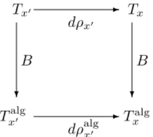
The terms in this expression are defined as follows. Let Tp denote the tangent

space at the point p (cf. 7.1.3, 7.1.6).

1. Let Ep ⊂ Tp be those elements for which there exists a representative

starting from p and contained completely in ΥCan.

2. Let p0 _{∈ C}0an _{such that φ}an_(p0_{) = p. The morphism φ}an _{induces a map}

dφp0 between the tangent spaces T_p0 and T_p(cf. 7.1.3, 7.1.6). Let e_p∈ E_p.

We define L(ep, p0) ⊂ Tp0 to be the preimages of e_p for the map dφ_p0. As

ΥC0an = (φan)−1(Υ_Can), any element of L(e_p, p0) can be represented by

a geodesic segment that is contained completely in ΥC0an. Let l(e_p, p0)

denote the cardinality of the set L(ep, p0).

3. We define np to be the cardinality of the set of preimages of the point p

i.e. np:= card{(φan)−1(p)}.

In Proposition 7.4.4, we show that w is indeed a well defined divisor whose degree is equal to 2g(ΥC0an) − 2. We then study the values n_p and l(e_p, p0)

described above. These results are sketched below.

We study the value np for p ∈ ΥCan in terms of two invariants - ram(p) and

c1(p) which are defined as follows.

(11)

1. If p is a point of type I then we set ram(p) to be the ramification degree ram(p0_{/p) for any p}0_{∈ C}0an _{such that φ}an_(p0_{) = p. As the morphism φ is}

Galois, ram(p) is well defined. If p is not of type I then we set ram(p) := 1. 2. In order to define the invariant c1, we introduce an equivalence relation

on C0_{(k). For y}

1, y2 ∈ C0(k), we set y1 ∼c(1) y2 if φ(y1) = φ(y2) and

ψ0_{(1, y}

1) = ψ0(1, y2). Let c1(y) denote the cardinality of the equivalence

class that contains y. In Lemma 7.4.8, we show that the function c1 :

C(k) → Z≥0 defined by setting c1(x) = c1(y) for any y ∈ φ−1(x) is well

defined. We proceed to show that if x ∈ C(k) then c1(x) depends only on

the point ψ(1, x) ∈ ΥCan. This defines c₁: Υ_Can→ Z_≥0.

The values c1(p) and ram(p) can be used to calculate npby the following relation

(Proposition 7.4.10).

np= [k(C0) : k(C)]/(c1(p)ram(p)).

We simplify the term l(ep, p0) which appears in the expression defining w.

Let p ∈ ΥCan and e_p ∈ E_p. In Lemma 7.4.12 we show that l(e_p, p0) remains

constant as p0 varies through the set of preimages p0 ∈ (φan₎−1_{(p). We set}

l(ep) := l(ep, p0). We introduce the invariants - ^ram(ep) and ram(p) to studyg

l(ep).

1. Let p ∈ ΥCan. By definition e_p is an element of the tangent space T_p

at p (cf. Sections 7.1.3, 7.1.6). As p is of type II, it corresponds to a discrete valuation of the ˜k-function field ]H(p). For any p0 _{∈ (φ}an₎−1_(p),

the extension of fields ]H(p) ,→ ^H(p0_{) can be decomposed into the}

com-posite of a purely inseparable extension and a Galois extension. Hence the ramification degree ram(e0_/e

p) is constant as e0varies through the set

of preimages of ep at Tp0 for the map dφalg

p0 : Tp0 → T_p (cf. 7.1.6). Let

g

ram(ep) be this number. When p is of type I, we setram(eg p) = ram(p)

and when p is of type III, we setram(e_g p) = c1(p).

2. For p ∈ ΥCan, we define ram(p) := Σg _e

p∈Ep1/ram(eg p).

In Proposition 7.4.15, we show that if p ∈ ΥCan and e_p∈ E_p then

l(ep) = [k(C0) : k(C)]/(npram(eg p)).

The results of Section 7.4 are compiled so that the value 2gan_(C0_{) − 2 can}

be computed in terms of the invariants c1,ram and ram.g

Theorem 7.4.17 Let φ : C0_{→ C be a finite morphism between smooth}

projec-tive irreducible k-curves such that the extension of function fields k(C) ,→ k(C0₎

induced by φ is Galois. Let gan_(C0_{) be as in Definition 7.1.25. We have that}

(12)

The results of chapter 7 form the content of the article ”A Riemann-Hurwitz formula for skeleta in non-Archimedean geometry”. Immediately following this work and related to it, were two papers ([ABBR1], [ABBR2]) by Amini, Baker, Brugall´e and Rabinoff wherein the authors study the extent to which morphisms between algebraic k-curves are determined by skeleta. Amongst the striking results of these papers, is the study of obstructions to the lifting of a harmonic morphism between metric graphs to a corresponding morphism of k-curves such that the graphs can be realized as skeleta of these curves. Also, a similar proof of Theorem 7.2.1 can be found in [ABBR1] (cf. Theorem A).

Recently, in [TEM2] and [TEM3], Michael Temkin, Adina Cohen and Dmitri Trushin have obtained results on wild ramification for finite morphisms between quasi-smooth Berkovich curves which bear some resemblance to results consid-ered in this paper. In [TEM3], Temkin considers a morphism f : Y → X be-tween connected separated quasi-smooth strictly k-analytic curves. The curves Y and X possess a natural metric and the morphism f is piecewise monomial on an interval I ⊂ Y with respect to this metric. The author is interested in the set Nf,≥d ⊂ Y of points y ∈ Y such that the multiplicity nf(y) of f at y is

at least d. The topologically tame case does not present a challenge as the set Nf,≥2 is contained in a finite graph and it is the topologically wild case which

is of greater interest. In [TEM2], the authors study the set Nf,≥p by using the

different. They show that the different function δf : Y → [0, 1] is piece-wise

monomial, relates the genus of Y and X and in addition completely controls the set Nf,p for morphisms of degree p. In [TEM3], Temkin goes on to prove

that the set Nf,≥d is radial with respect to a large enough skeleton of f (a

compatible choice of skeleta Υ0 ⊂ Y and Υ ⊂ X) and that their Υ0_{-radii are}

piece-wise |k∗|-monomial functions on Υ0_{. The author then relates the radii of}

Nf,≥d to classical ramification invariants.

1.2 Finite morphisms and skeleta

Our second set of results concerns finite surjective morphisms between irre-ducible projective varieties over non-Archimedean real valued fields. We study such morphisms in terms of the morphisms they induce between the analytifica-tions of the varieties. The theorem we prove implies that the induced morphism when viewed as a continuous map between topological spaces admits a certain uniform behaviour. Before stating the theorem in full generality, we provide its motivation by considering the case of a finite endomorphism of the projective line.

Let k be an algebraically closed, complete non-Archimedean real valued field whose value group |k∗_{| contains at least two elements and is a sub group of}

(R>0, ×). Let P1,ank be the Berkovich analytification of the projective line P1k.

The analytification P1,an_k allows us to use the valuative topology provided by the field to study an algebraic endomorphism. For a point x ∈ P1

k(k) ⊂ P 1,an k ,

we have the notion of a Berkovich closed disk or Berkovich open ball centred at x within the space P1,an_k which contains the naive closed or open disk around x. By the naive closed (open) disk around x ∈ k of radius r ∈ R>0, we mean the set

{y ∈ k||y−x| ≤ r} ({y ∈ k||y−x| < r}). As opposed to their naive counterparts, the Berkovich open and closed disks are locally compact and contractible.

(13)

Let φ : P1

k → P1k be a finite morphism. For a complete non-Archimedean

real valued algebraically closed field extension L/k, let φLdenote the morphism

φ × idL: P1k×kSpec(L) → P1k×kSpec(L).

The analytification of a k-variety of finite type (cf. Section 5.6) is functorial and hence endomorphisms of the projective line will induce endomorphisms of its analytification. That is, the morphism φ induces a morphism

φan_{: P}1,an k → P

1,an k .

The morphism φan

L is similarly defined and it is to be noted that φanL = φan×id an L .

Our reason for introducing the morphism φLfor a complete non-Archimedean

real valued algebraically closed field extension L/k is to deal with all points of the analytification of the projective line over k and not just those points for which H(x) = k (cf. 5.6.2). When discussing the points of the analytification of a k-variety, we make use of the description outlined in Section 5.6. Let x ∈ P1,an_k (L) i.e. x ∈ P1,an _{and there exists an embedding of valued fields H(x) ,→ L. The}

image of x ∈ P1,an_k (L) for the morphism π : P1,an_k → P1

k (cf. 5.6) is an L-point of

P1

k i.e. an element of the set P1k(L). We abuse notation and refer to this point

as x as well. The pair x : Spec(L) → P1

k and idL: Spec(L) → Spec(L) defines

a closed point of the variety P1

k×kSpec(L) which we denote xL. The following

remark generalizes this construction.

Remark 1.2.1. Let V be a k-variety and let x ∈ Van_{. The field H(x) is the}

non-Archimedean geometry analogue of the residue field of a point in algebraic geometry and is defined in 5.6. Let L be a complete non-Archimedean real valued algebraically closed field extension of k. The notation x ∈ Van_{(L) will be used}

to mean that x ∈ Van_{and in addition there exists an embedding of valued fields}

H(x) ,→ L. It follows that the image of the point x for the morphism Van_{→ V}

which is defined in Section 5.6 is an L-point i.e. an element of the set V (L). We abuse notation and refer to this point as x as well. The pair x : Spec(L) → V and idL: Spec(L) → Spec(L) defines a closed point of the variety V ×kSpec(L)

which we denote xL. This construction will be referred to frequently in what

follows.

We now introduce the theorem concerning finite endomorphisms of the pro-jective line over k.

Theorem 1.2.2. Let φ : P1

k→ P1k be a finite morphism. Let x ∈ P 1,an

k and L/k

be any complete non-Archimedean real valued algebraically closed field extension of k such that x ∈ P1,ank (L). Let f (x) be the minimum of 1 and the radius of

the largest Berkovich open ball B ⊂ P1,an_L around xL ∈ P1L(L) ⊂ P 1,an L whose

preimage under φan

L is the disjoint union of homeomorphic copies of B via φanL.

The function f : P1,an_k → R≥0 is not identically zero and well defined. There

exists a finite simplicial complex Υ ⊂ P1,an_k , a generalised real interval I := [i, e] and a deformation retraction

ψ : I × P1,an_k → P1,an_k

such that ψ(e, P1,an_k ) = Υ and the function f is constant on the fibres of this retraction i.e. for every x ∈ P1,an_k we have that f (x) = f (ψ(e, x)). Furthermore, the function logc|f | is piecewise linear when restricted to Υ where 0 < c < 1 is

(14)

Remark 1.2.3. We fix the real number c which appears in the portion of the theorem above concerning piecewise linearity and hence forth write log(|f |) in place of logc(|f |).

The notion of a generalised interval is discussed in Section 3.9 [HL]. We now provide an example which illustrates the behaviour of the function f in Theorem 1.2.2 clearly.

Example 1.2.4. Let k be an algebraically closed complete non-trivially val-ued non-Archimedean field which is of characteristic p. Consider the morphism φ : P1

k → P1k given by z 7→ zp− z. Let L/k be a non-Archimedean real valued

field extension. The morphism φL is ´etale over every point other than ∞.

Fur-thermore it can be shown that f (x) = 1 if x 6= ∞ and 0 at ∞. Let Υ be a finite graph containing the point ∞ and which contains at least one other point. Since there is a deformation retraction of P1,ank onto any non - empty finite sub-graph,

it follows that there exists a deformation retraction ψ : I × P1,an_k → P1,an_k

such that the function f is constant along the fibres of the retraction.

Our first goal is to generalize Theorem 1.2.2 to the case of finite surjective morphisms between irreducible, projective varieties. A problem standing in the way of any attempt at a generalisation is that there is no intrinsic notion of an open disk in Van _{if V is a projective k-variety of finite type. However, as V is}

projective there exists a closed immersion V ,→ Pn

k for some n ∈ N. We identify

V with its image under the closed immersion. The space Pn,an_k can be equipped with a finite formal cover [[B], Section 4.3] such that each element of this cover is isomorphic to the n-dimensional Berkovich closed disk M(k{T1, . . . , Tn}).

Let {Ai}i denote this cover. The intersection of the elements of the formal

cover with the image of the immersion Van ,→ Pn,ank defines a formal cover of

the space Van_{, namely {A}

i∩ Van}i. Furthermore, for a non-Archimedean real

valued algebraically closed field extension L/k the construction extends to the analytic space (VL)an:= (V ×kL)an. The n - dimensional Berkovich open balls

contained in Pn,an_L allow us to generalise Theorem 1.2.2. We now provide a sketch of the details of this construction.

Let L/k be a non-Archimedean real valued algebraically closed field exten-sion and x ∈ Pn,an_L (L) (Remark 1.1). Let i be such that xL∈ Ai,L. Associated

to the point xL is a collection of open neighbourhoods in Pn,anL (L), namely the

Berkovich open balls around xL contained in Ai,L. We denote this family of

open neighbourhoods OxL. Let G ∈ OxL. For every j such that xL belongs

to Aj,L, it can be checked that G is a Berkovich open ball in Aj,L as well.

This implies that the family OxL is independent of the element of the affinoid

chart which contains xL and is hence well defined. We now define a poly

ra-dius associated to the elements of OxL. Let xL have homogenous coordinates

[x1,L : . . . : xn+1,L] and let W ∈ OxL. We can associate an (n + 1)

2_-tuple

denoted hL(W ) to the open neighbourhood W as follows. If for an index t,

xL ∈ At,L then let rt = (r1, . . . , rn+1) be such that rt = 1 and the Berkovich

open ball BW,tis defined by the equations |(Tj/Tt−xj,L/xt,L)(p)| < rj for j 6= t.

If on the other hand xL does not belong to At,L then let rt = (1, . . . , 1). We

define hL(W ) := (rt)t. Let OL :=Sx∈Pn,an

(15)

construction to define a function hL : OL → R(n+1)

2

≥0 . Note that the sets OxL

depend on the affine chart chosen for Pn_{. In the case of P}1

k with x ∈ P 1,an k (L),

the set OxL associated to the construction above is discussed in Section 8.1. In

what follows we explain how the family OL can be ordered.

Remark 1.2.5. We introduce a collection S of functions from R(n+1)_>0 2 to R>0.

The set S consists of those functions g : R(n+1)>0 2 → R>0 which satisfy the

following properties.

1. The function g is continuous.

2. If (ri,j)i,j and (si,j)i,j are (n + 1)2-tuples such that ri,j ≤ si,j for all i, j

then g((ri,j)i,j) ≤ g((si,j)i,j).

3. g is a definable function (in the model theoretic sense) in the language of Ordered Abelian groups.

Let g ∈ S. The function g defines a total ordering on the set R(n+1)>0 2 as

follows. Let r, s ∈ R(n+1)_>0 2. We set r ≤gsif g(r) ≤ g(s). Observe that the total

ordering ≤gon R(n+1)

2

>0 extends the partial ordering given by : (ri,j)i,j≤ (si,j)i,j

if ri,j ≤ si,j for all i, j, where (ri,j)i,j and (si,j)i,j are R(n+1)

2

>0 tuples.

We can extend g to a function ˜g : R(n+1)_≥0 2 → R≥0 as follows. For r ∈

R(n+1)2 >0 , we set ˜g(r) := g(r) and if r ∈ R (n+1)2 ≥0 r R (n+1)2 >0 then ˜g(r) := 0. As for

g, the function ˜g defines a total ordering on R(n+1)_≥0 2 which extends the partial ordering given by : (ri,j)i,j≤ (si,j)i,j if ri,j ≤ si,j for all i, j, where (ri,j)i,j and

(si,j)i,j are R(n+1)

2

≥0 tuples. Henceforth, we abuse notation and write g for the

extension ˜g.

Let g ∈ S. By Lemma 8.1.2, the function g◦hL : OL→ R≥0has the following

property. If O1, O2∈ OL such that O1⊆ O2 then (g ◦ hL)(O1) ≤ (g ◦ hL)(O2).

The functions g ∈ S hence allow us to quantify the size of elements belonging to OL.

We now provide an equivalent form of Theorem 1.2.2 which we generalize. We begin by motivating the reformulation. The goal of Theorem 1.2.2 is to prove the existence of a finite simplicial complex Υ contained in P1,an_k such that the function f is constant along the fibres of the retraction morphism ψ(e, ). Let us assume that Theorem 1.2.2 is true. We define a function M : Υ → R≥0

as follows. Let γ ∈ Υ and x ∈ P1,an_k be any point for which ψ(e, x) = γ. We set M (γ) := f (x). Let L/k be any complete non-Archimedean real valued algebraically closed field extension such that x ∈ P1,an_k (L). By definition M (γ) is the minimum of 1 and the radius of the largest Berkovich open ball in P1,anL

around xL whose preimage is the disjoint union of homeomorphic copies of

itself for the morphism φan

L. The function M is well defined since we assumed

Theorem 1.2.2 is true. Hence a suitable restatement of 1.2.2 is the following theorem.

Theorem 1.2.6. Let φ : P1

k → P1k be a finite morphism. There exists a

gener-alised real interval I := [i, e] and a deformation retraction ψ : I × P1,an_k → P1,an_k

(16)

which satisfies the following properties.

1. The image ψ(e, P1,an_k ) of the deformation retraction ψ is a finite simplicial complex. Let Υ denote this finite simplicial complex.

2. There exists a well defined function M : Υ → [0, 1] which satisfies the following conditions. The function M is not identically zero and log(M ) is piecewise linear. Let γ ∈ Υ such that M (γ) > 0 and x ∈ ψ(e, )−1_(γ).

Let L/k be any complete non-Archimedean real valued algebraically closed field extension such that x ∈ P1,an_k (L). Then the following are true.

(a) The preimage under the morphism φan

L of the Berkovich open ball

B(xL, M (γ)) ⊂ P1,anL around xL of radius M (γ) decomposes into

the disjoint union of Berkovich open balls each homeomorphic to B(xL, M (γ)) via the morphism φanL.

(b) Let O be any other Berkovich open ball around xL whose radius is

less than or equal to 1 such that its preimage under the morphism φan

L decomposes into the disjoint union of Berkovich open balls each

homeomorphic to O via φan

L. Then the radius of O must be less than

or equal to M (γ).

We will show that Theorems 1.2.2 and 1.2.6 are equivalent in Section 8.2.1. We now state a theorem which in Section 8.5 we will show to be a general-isation of Theorem 1.2.2. Let φ : V0 → V be a finite surjective morphism between irreducible, projective varieties of finite type over k. For a complete non-Archimedean real valued algebraically closed field extension L/k, let φL

denote the morphism

φ × idL: V ×kL → V ×kL.

As in the case of P1

k, we write φan : V0an → Van for the induced morphism

between the respective analytifications. The morphism φan

L is similarly defined

and it is to be noted that φan

L = φan× idanL. We fix an embedding V ,→ Pnk and

an affine chart of Pn_{. The theorem will be stated in terms of the sets O} xL and

the functions hL and g described above.

Theorem 8.4.3. Let φ : V0 → V be a finite surjective morphism between irreducible, projective varieties with V normal. Let g ∈ S. There exists a generalized real interval I := [i, e] and a deformation retraction

ψ : I × Van_{→ V}an

which satisfies the following properties.

1. The image ψ(e, Van_{) of the deformation retraction ψ is a finite simplicial}

complex which we denote Υg.

2. There exists a well defined function Mg : Υg → R≥0 which satisfies the

following conditions. The function Mg is not identically zero. Let γ ∈

Υg be a point on the finite simplicial complex for which Mg(γ) 6= 0 and

x ∈ ψ(e, )−1(γ). Let L/k be any complete non-Archimedean real valued algebraically closed field extension such that x ∈ Van_{(L). There exists}

(17)

W ∈ (g ◦ hL)−1(Mg(γ)) ∩ OxL such that the open set (φ

an

L)−1(W ∩ VLan) ⊂

V0an

L decomposes into the disjoint union of open sets, each homeomorphic

to W ∩ Van

L via φanL . Furthermore, let O ∈ OxL be such that the preimage

of O ∩ Van

L under φanL decomposes into the disjoint union of open sets in

V0an

L , each homeomorphic to O via the morphism φanL . Then (g ◦ hL)(O) ≤

Mg(γ). Lastly, the function log(Mg) is piecewise linear on Υg.

Remark 1.2.7. The second property we require the function Mg to satisfy

in-volves choosing a point xL over x which is an L-point of VLanand then requiring

that Mg fulfill a condition concerning xL. It may hence seem that the function

is dependent on the field L chosen. However, showing that the function Mg is

well defined implies in particular that the value Mg(x) for x ∈ Vanis determined

entirely by x.

It is worth mentioning that the result stated above when applied to smooth Berkovich analytic curves over a field of characteristic zero bears some similarity with theorems proved in [PP] and [Bal]. In [Bal], the author - F. Baldassarri studies a system of differential equations defined over an analytic domain of the affine line over a non-Archimedean real valued field of characteristic zero. More precisely, let k be a non-Archimedean field of characteristic zero and X be a relatively compact analytic domain of the affine line A1,an_k . Let

Σ : dy/dT = Gy

be a system of linear differential equations where G is a µ×µ matrix of k-analytic functions on X. If x ∈ X is a k-rational point, let R(x) = R(x, Σ) denote the radius of the maximal open disk in X with center at x on which all solutions of Σ converge. The author shows that the function R is continuous. Also, he illustrates how when X = A1,ank there exists a finite graph Γ ⊂ A

1,an k which

controls the behaviour of the function R. Since A1,ank retracts to any of its finite

subgraphs, this means that the function R is constant along the fibres of the retraction on Γ. In the paper the control by a finite graph is illustrated by an example. If one preserves the restrictions on the field k and considers the case of a system of differential equations defined instead over a smooth Berkovich curve then a similar result holds true. In [PP], the authors - Poineau and Pulita prove that associated to a system of differential equations over a smooth Berkovich curve, there exists a locally finite graph contained in the curve and a retraction of the curve onto it such that the radius of convergence function is constant along the fibres of the retraction. The results we prove and the results of Poineau-Pulita and Baldassari show that the behaviour of certain functions of interest are controlled by finite simplicial complexes associated to them. Notation : To prove the main theorems that follow, we require techniques from Model theory where it is standard to write the value group of a non-Archimedean valued field additively. However, when discussing objects from Berkovich geom-etry such as affinoid algebras and the reduction morphism it is standard to endow the value group with a multiplicative structure as it aids in intuition. Instead of resolving this dichotomy in notation, we preserve both notation and eliminate ambiguity by specifying at every instance the structure of the value group, i.e. whether we look at it additively or multiplicatively.

(18)

Chapter 2

Introduction en fran¸

cais

Les corps non-archimédiens ont été découverts au début du vingtième siècle, lorsque K. Hensel a défini le corps des nombres p-adique. Dans les années qui suivirent, on observa plusieurs tentatives, chacune ayant ses mérites, de développement d’une théorie géométrique sur ces corps comparable a celle développée sur le corps des nombres complexes. Cependant, ce n’est qu’au début des années 90 que Vladimir Berkovich introduit une théorie de la géométrie non-archimédienne qui nous fourni des espaces analytiques possédant les bonnes propriétés topologiques. Dans le cadre de cette théorie, on peut associer un espace analytique au sens de Berkovich à une variété définie sur un corps non-archimédien. On appelle cet espace analytique l’analytification de la variété. Même si une variété sur un corps non-archimédien est totalement discontinue pour la topologie induite par la valuation du corps, son analytification est Haus-dorff, localement compacte avec un nombre fini de composantes connexes par arcs. Ainsi, il semble naturel d’étudier le type d’homotopie de l’analytification de telles variétés.

En 2010, Hrushovski et Loeser ont utilisé la théorie des modèles pour étudier le type d’homotopie de l’analytification d’une variété sur un corps non-archimédien non-trivialement valué. Ils ont montré que les types d’homotopie sont com-pletement déterminé par certains complexes simpliciaux contenus dans les an-alytifications. Plus précisément, étant donné une variété sur un corps non-archimédien, ils ont construit une rétraction par déformation de l’analytification de la variété sur un complexe simplicial contenu dans l’analytification. Dans [HL], Hrushovski et Loeser ont introduit l’espace chapeauté associé à une variété qui est la version analogue dans la théorie des modèles de l’analytification. Un des avantages de ce point de vu est le fait qu’on peut parler des notions de définissabilité et également utiliser les méthodes puissantes comme compacité. Cette thèse reflète et s’appuie sur cette interaction entre la théorie des modèles et la géométrie de Berkovich. Nous montrerons que plusieurs phénomènes topologiques concernant des analytifications de variétés sont contrôlés par cer-tains complexes simpliciaux contenus dans les analytifications.

(19)

2.1 Une formule de Riemann-Hurwitz pour le

genre analytique

Soit k un corps alg´ebriquement clos et complet pour une valuation non-archim´edienne `

a valeurs réelles et non-triviale. Soit C une courbe sur k. Par une courbe sur k, on veut dire un k-schéma réduit, connexe et séparé de dimension 1. Il est bien connu qu’il existe une rétraction par déformation de l’analytification Can

de C sur un sous-ensemble fermé Υ qui est homéomorphe à un graphe fini [[B], Chapter 4], [[HL], Section 7]. Ces types des sous-espaces sont appelés squelettes. Le squelette Υ peut-être décomposé en un ensemble des sommets V (Υ) et un ensemble d’arêtes E(Υ). On définit le genre du graphe Υ par l’équation suivante.

g(Υ) = 1 − V (Υ) + E(Υ).

Dans la Proposition 7.1.24, nous montrons que g(Υ) est un invariant bien d´efini de la courbe. Soit gan_{(C) := g(Υ) pour un tel squelette Υ. Nous ´etudions}

le comportement de l’invariant gan_{pour un morphisme fini en utilisant une paire}

de r´etractions compatibles.

Soit φ : C0 _{→ C un morphisme fini entre deux courbes projectives, lisses et}

irr´eductibles. Le morphisme φ va induire un morphisme φan_{: C}0an_{→ C}an_entre

les deux analytifications. Nous démontrons qu’il existe une paire compatible de rétractions par déformations

ψ : [0, 1] × Can→ Can

et

ψ0: [0, 1] × C0an→ C0an avec les propri´et´es suivantes:

1. Les ensembles ΥC0an := ψ0(1, C0an) et Υ_Can := ψ(1, Can) sont des

sous-espaces fermés de C0an_{et C}an_{. Ils sont homéomorphes à des graphes finis.}

De plus, on a l’´egalit´e ΥC0an = (φan)−1(Υ_Can).

2. Les espaces analytiques C0anr ΥC0an et Canr Υ_Can se d´ecomposent en

une union disjointe de copies de disques unit´es de Berkovich i.e. il existe deux ensembles de sommets faiblement semi-stables (cf. Definition 7.1.18) A⊂ Can_{et A}0 _{⊂ C}0an _{tel que Υ}

Can = Σ(Can, A) et Υ_C0an= Σ(C0an, A0).

3. Les r´etractions par d´eformations ψ and ψ0 sont compatibles, cela veut dire que le diagramme suivant est commutatif.

(20)

[0, 1] × Can _Can [0, 1] × C0an _C0an ? ? -ψ ψ0 id × φan _φan

Les notations utilisées pour le résultat suivant sont explicitées dans la Sec-tion 7.3.1 et les définiSec-tions 7.3.6 et 7.3.8.

Corollaire 7.3.9 Soit φ : C0 → C un morphisms s´eparable fini entre deux courbes lisses et projectives sur le corps k. Soit gan_(C0_{), g}an_{(C) les invariants}

d´efinis dans la Definition 7.1.25. On a l’´equation suivante.

2gan(C0) − 2 = deg(φ)(2gan(C) − 2) + Σp∈Can2i(p)g_p+ R − Σ_p∈CanR1

p.

Dans la Section 7.4, on propose une autre méthode pour calculer l’invariant gan_(C0_{) en utilisant l’existence de la paire de rétractions par déformations ψ}

et ψ0 _{sur C}an _{et C}0an _{dont les images sont des squelettes Υ}

Can et Υ_C0an. On

suppose ´egalement que le morphisme φ : C0 _{→ C est tel que l’extension du}

corps des fonctions k(C) ,→ k(C0_{) est Galois. Par construction de ψ}0 _{et ψ, φ}an

induira un morphisme entre les deux squelettes. Nous montrons que le genre du squelette ΥC0an peut être calculé en utilisant certains invariants associés aux

points de ΥCan. On d´efinit un diviseur w sur Υ_Can de degr´e 2g(Υ_C0an) − 2. Un

diviseur sur un graphe fini est un élément du groupe abélien libre engendré par les points du graphe.

Le diviseur w est d´efini comme suit. Pour un point p ∈ ΥCan, soit w(p)

l’ordre du diviseur au point p. Soit

w(p) := ( X

ep∈Ep,p0∈(φan)−1(p)

l(ep, p0)) − 2np.

Les termes dans cette expression sont d´efinis comme suit. Soit Tp l’espace

tangent au point p (cf. 7.1.3, 7.1.6).

1. Soit Ep⊂ Tpl’ensemble des éléments pour lesquels il existe un représentant

`

a partir de p contenu dans ΥCan.

2. Soit p0_{∈ C}0an_{tel que φ}an_(p0_{) = p. Le morphisme φ}an_{induit un morphisme}

dφp0 entre les espaces tangents T_p0 et T_p (cf. 7.1.3, 7.1.6). Soit e_p ∈ E_p.

On d´esigne par L(ep, p0) ⊂ Tp0 l’ensemble des pr´eimages de e_p pour le

morphisme dφp0. Comme Υ_C0an = (φan)−1(Υ_Can), un ´el´ement de L(e_p, p0)

peut être représenté par un segment géodésique contenu dans ΥC0an. Soit

(21)

3. On désigne par np la cardinalité de l’ensemble des préimages du point p

i.e. np:= card{(φan)−1(p)}.

Dans la Proposition 7.4.4, nous montrons que w est un diviseur bien défini de degré 2g(ΥC0an) − 2. Puis, nous étudions les invariants n_p et l(e_p, p0) de la

mani´ere suivante.

On ´etudie l’invariant nppour p ∈ ΥCanen termes de deux invariants - ram(p)

et c1(p) qui sont d´efinis comme suit.

Soit p ∈ ΥCan.

1. Si p est un point de type I, on d´esigne par ram(p) le degr´e de ramification ram(p0/p) pour tout p0 ∈ C0an _{tel que φ}an_(p0_{) = p. Comme le morphisme}

φ est Galois, ram(p) est bien d´efini. Si p n’est pas de type I, on d´efinit ram(p) := 1.

2. Afin de d´efinir l’invariant c1, nous introduisons une relation d’´equivalence

sur C0_{(k). Soient y}

1, y2 ∈ C0(k). Nous d´efinissons y1 ∼c(1) y2 si φ(y1) =

φ(y2) et ψ0(1, y1) = ψ0(1, y2). On d´esigne par c1(y) la cardinalit´e de la

classe d’´equivalence qui contient y. Dans le Lemme 7.4.8, nous montrons que la fonction c1 : C(k) → Z≥0 donn´ee par c1(x) = c1(y) pour tout

y ∈ φ−1_{(x) est bien d´efinie. Nous montrons que c}

1(x) pour x ∈ C(k) ne

d´epend que du point ψ(1, x) ∈ ΥCan. Ceci d´efinit c₁: Υ_Can→ Z_≥0.

Les valeurs c1(p) et (p) peuvent être utilisées pour calculer np via l’équation

suivante (Proposition 7.4.10).

np= [k(C0) : k(C)]/(c1(p)ram(p)).

Nous simplifions le terme l(ep, p0). Soit p ∈ ΥCan and e_p ∈ E_p. Dans

le Lemme 7.4.12, nous montrons que l(ep, p0) est constant pour tout p0 ∈

(φan₎−1_{(p). On d´efinit l(e}

p) := l(ep, p0). Nous introduisons les invariants

-^

ram(ep) etram(p) pour ´etudier l(eg p).

1. Soit p ∈ ΥCan. Par définition, e_pest un élément de l’éspace tangent T_p à p

(cf. Sections 7.1.3, 7.1.6). Comme p est de type II, ¸ca correspond `a une val-uation discr`ete du ˜k-corps des fonctions ]H(p). Pour tout p0_{∈ (φ}an₎−1_(p),

l’extension de corps ]H(p) ,→ ^H(p0_{) peut être décomposée en une extension}

ins´eparable et une extension Galoisienne. Ainsi, le degr´e de ramification ram(e0_/e

p) est constant pour tous les pr´eimages

de ep pour le morphisme dφalgp0 : Tp0 → T_p (cf. 7.1.6). On d´esigne par

g

ram(ep) ce degr´e de ramification. Si p est un point de type I, on d´efinit

g

ram(ep) := ram(p) et si p est de type III, on d´efinitram(eg p) = c1(p).

2. Pour tout p ∈ ΥCan, on d´efinit ram(p) := Σg _e

p∈Ep1/ram(eg p).

Soit p ∈ ΥCan et e_p∈ E_p. Dans la Proposition 7.4.15, nous montrons que

(22)

On peut résumer l’ensemble des résultats de la Section 7.4 par le résultat suivant où on calcule la valeur 2gan_(C0_{) − 2 en termes des invariants c}

1,ram etg

ram.

Theoreme 7.4.17 Soit φ : C0_{→ C un morphisme fini entre deux courbes lisses}

projectives et irr´eductibles tels que l’extension du corps des fonctions k(C) ,→ k(C0) induite par φ est Galoisienne. Soit gan_(C0_{) le genre analytique de la}

Definition 7.1.25. On a l’´equation suivante.

2gan(C0) − 2 = deg(φ)Σp∈ΥCan[ram(p) − 2/(cg 1(p)ram(p))].

2.2 Morphismes finis et squelettes

La deuxième série de résultats dans cette thèse concerne les morphismes finis sur-jectifs entre des variétés projectives irréductibles sur un corps non archimédien. On étudie un tel morphisme en termes du morphisme induit entre les analytifi-cations. Le théorème principal (Theorem 8.4.3) implique que le comportement de ce morphisme entre les analytifications est modéré. Avant de le préciser, nous donnons la motivation en considérant le cas d’un endomorphisme de la droite projective.

Soit k un corps algébriquement clos complet pour une valuation non triv-iale à valeurs réelles. Soit φ : P1,an_k → P1,an_k un morphisme fini. Comme l’analytification dans le sens de Berkovich d’un morphisme est une construc-tion fonctorielle, le morphisme φ induit un morphisme φan_{: P}1,an

k → P 1,an k entre

les deux analytifications. Pour un point x ∈ P1

k(k) ⊂ P 1,an

k , on a la notion de

boule fermée de Berkovich ou de boule ouverte de centre x et contenue dans l’éspace P1,an_k . Une boule fermé (ouverte) de Berkovich de centre x contient la boule fermée (ouverte) na¨ıve de centre x. On désigne par la boule fermée (ouverte) na¨ıve de centre x et rayon r, l’ensemble des points {y ∈ k||y − x| ≤ r} ({y ∈ k||y − x| < r}). Les boules de Berkovich sont localement compactes et contractiles.

Pour une extension L/k non archimédienne algébriquement close complète, on désigne par φL le morphisme

φ × idL: P1k×kSpec(L) → P1k×kSpec(L).

Le morphisme φan

L est d´efini comme avant et il faut noter que φanL = φan× id an L .

Les morphismes φLnous permettent de traiter tous les points de l’analytification

de la droite projective et pas seulement les points pour lesquels H(x) = k (cf. 5.6.2). Lorsque l’on parle des points de l’analytification d’une vari´et´e sur k, on utilise la description de Section 5.6. Soit x ∈ P1,an_k (L) i.e. x ∈ P1,an _{et il existe}

une immersion de corps valu´es H(x) ,→ L. L’image du point x ∈ P1,an_k (L) pour le morphisme π : P1,an_k → P1

k (cf. 5.6) est un L-point de P1k i.e. un ´el´ement

de l’ensemble P1

k(L) que l’on d´esigne aussi par x. La paire x : Spec(L) → P1k

(23)

désigné par xL. La remarque suivante généralise cette construction.

Remark 1.1. Soit V une vari´et´e sur k et soit x ∈ Van_{. Le corps H(x) (cf.}

Section 5.6) est la version non archimédienne du corps résiduel d’un point en géométrie algébrique. Soit L une extension non archimédienne complète de k. La notation x ∈ Van_{(L) veut dire que x ∈ V}an _{et qu’il existe une immersion de}

corps valués H(x) ,→ L. On peut en déduire que l’image du point x pour le mor-phisme Van_{→ V qui est défini dans Section 5.6 est un L-point i.e. un élément}

de l’ensemble V (L) que l’on désigne aussi par x. La paire x : Spec(L) → V et idL : Spec(L) → Spec(L) définit un point fermé de la variété V ×kSpec(L)

qu’on d´esigne par xL. On utilisera cette construction dans la Section 8.

Nous introduisons maintenant le th´eor`eme concernant un endomorphisme fini de la droite projective sur k.

Theorem 1.2.2. Soit φ : P1

k → P1k un morphisme fini. Soit x ∈ P 1,an k et L/k

une extension algébriquement close non archimédienne valuée et complète telle que x ∈ P1,an_k (L). Soit f (x) le minimum de 1 et du rayon de la plus grande boule ouverte de Berkovich de centre xL∈ P1L(L) ⊂ P

1,an

L dont l’image r´eciproque pour

le morphisme φan

L est union disjointe de copies hom´eomorphes de B via φanL. La

fonction f : P1,an_k → R≥0 n’est pas identiquement 0 et elle est bien d´efinie.

Il existe un complexe simplicial fini Υ ⊂ P1,ank , un intervalle réel généralisé

I := [i, e] et une r´etraction par d´eformation ψ : I × P1,an_k → P1,an_k

tels que ψ(e, P1,an_k ) = Υ et la fonction f soit constante le long des fibres de la rétraction i.e. pour tout x ∈ P1,an_k , f (x) = f (ψ(e, x)). De plus, la restriction sur Υ de la fonction logc|f | est linéaire par morceaux où 0 < c < 1 est un nombre

r´eel.

Remark 1.3. Nous fixons le nombre réel c qui apparaˆıt dans le Théorème 1.2.2 et désignons par log(|f |) la fonction logc(|f |).

La notion d’intervalle réel généralisé est défini dans la Section 3.9 de [HL]. Nous donnons maintenant un exemple pour comprendre le comportement de la fonction f du Théorème 1.2.2.

Example 1.3. Soit k un corps algébriquement clos complet et non archimédien de caractéristique p. Considèrons le morphisme φ : P1

k → P1k d´efini par z 7→

zp_{−z. Soit L/k une extension non archim´edienne valu´ee. Le morphisme φ} L est

étale au-dessus tous les points sauf ∞. On peut vérifier que f (x) = 1 si x 6= ∞ et f (∞) = 0. Soit Υ un graphe fini qui contient le point ∞ et au moins un autre point de P1,an_k . Comme il existe une rétraction par déformation de P1,an_k sur tout sous-graphe fini et non-vide, on en déduit l’existence d’une rétraction par déformation

ψ : I × P1,an_k → P1,an_k

(24)

Notre but premier est de généraliser le Théorème 1.2.2 au cas d’un mor-phisme fini surjectif entre des variétés irréductibles et projectives. Un des ob-stacles à une telle généralisation est le fait qu’il n’y a pas de notion intrinsèque de boule ouverte dans Van_{si V est une variété projective sur k de type fini.}

Cepen-dant, comme V est projective, il existe une immersion ferm´ee V ,→ Pn

k o`u n ∈ N.

Nous identifions V avec son image sous cette immersion fermée. On peut im-poser sur Pn,an_k un recouvrement formel [[B], Section 4.3] tel que chaque élément dans ce recouvrement soit isomorphe à la boule fermée de Berkovich de dimen-sion n, M(k{T1, . . . , Tn}). On désigne par {Ai} ce recouvrement. L’intersection

des ´el´ements de ce recouvrement avec l’image de l’immersion Van _{,→ P}n,an k

d´efinit un recouvrement formel de l’espace Van_{, notamment {A}

i∩ Van}i. En

outre, pour une extension non archimédienne valuée et algébriquement close L/k, la construction s’étend à l’espace analytique (VL)an := (V ×k L)an. Les

boules de Berkovich de dimension n contenues dans Pn,anL nous permettent de

généraliser le Théorème 1.2.2. Voici les détails de cette construction.

Soit L/k une extension de corps alg´ebriquement close et non archim´edienne. Soit x ∈ Pn,an_L (L) (Remark 1.1). Soit i ∈ {1, . . . , n + 1} tel que xL ∈ Ai,L.

La famille des boules ouvertes de Berkovich de centre xL et contenues dans

Ai,L, d´efinit une collection de voisinages ouverts de xL dans Pn,anL (L). On

d´esigne par OxL cette famille des voisinages. Soit G ∈ OxL. Pour chaque j

tel que xL∈ Aj,L, on peut v´erifier que G est une boule de Berkovich contenue

dans Aj,L. Cela implique que la famille OxL ne dépend pas de l’élément de

récouvrement formel qui contient xLet on déduit que OxL est bien défini. Nous

définissons le polyrayon d’un élément de la famille OxL. Supposons que le point

xL a pour cordonn´ees homog`enes [x1,L : . . . : xn+1,L] et W ∈ OxL. On peut

lui associer un ´el´ement hL(W ) de Rn+1

2

`a W comme suit. Si xL ∈ At,L pour

t ∈ {1, . . . , n + 1}, on d´efinit rt:= (r1, . . . , rn+1) o`u rt= 1 et la boule ouverte

de Berkovich BW,t est d´efinie par les ´equations |(Tj/Tt− xj,L/xt,L)(p)| < rj

pour j 6= t. Si xL ∈ A/ t,L, on d´efinit rt := (1, . . . , 1). Soit hL(W ) := (rt)t et

OL :=Sx∈Pn,an_k (L)OxL. On peut ´etendre cette construction pour obtenir une

fonction hL: OL→ R(n+1)

2

≥0 . Il faut noter que la famille OxL d´epend de la carte

affine de Pn qu’on avait choisi. Dans le cas de P1k avec x ∈ P 1,an

k (L), la famille

OxL obtenue par cette construction est analys´ee dans la Section 8.1. Dans ce

qui suit, nous expliquons comment imposer un ordre sur la famille OL.

Remark 1.5.

Nous introduisons une famille S des fonctions de R(n+1)_>0 2 `a R>0. L’ensemble

S se compose des fonctions g : R(n+1)

2

>0 → R>0 qui satisfont les propri´et´es

suivantes.

1. La fonction g est continue. 2. Si (ri,j)i,j, (si,j)i,j ∈ Rn+1

2

sont tels que ri,j ≤ si,j pour tout i, j, on a

l’in´egalit´e g((ri,j)i,j) ≤ g((si,j)i,j).

3. La fonction g est définissable dans le langage des groupes Abéliennes or-donnés.

(25)

suit. Soit r, s ∈ R(n+1)>0 2. Nous d´efinissons r ≤g ssi g(r) ≤ g(s). Il faut noter

que l’ordre total ≤g sur R(n+1)

2

>0 est donn´e par (ri,j)i,j ≤ (si,j)i,j si ri,j ≤ si,j

pour tout i, j o`u (ri,j)i,j, (si,j)i,j ∈ R(n+1)

2

>0 .

On peut ´etendre g pour obtenir une fonction ˜g : R(n+1)_≥0 2 → R≥0 comme

suit. Pour tout r ∈ R(n+1)>0 2, on d´efinit ˜g(r) := g(r) et si r ∈ R (n+1)2

≥0 r R (n+1)2

>0

on suppose ˜g(r) := 0. Comme pour la fonction g, ˜g définit un ordre total sur R(n+1)_≥0 2 qui étend l’ordre partiel donné par (ri,j)i,j≤ (si,j)i,j si ri,j≤ si,j pour

tout i, j o`u (ri,j)i,j, (si,j)i,j ∈ R(n+1)

2

≥0 . Dans ce qui suit, on utilise g `a la place

de l’extension ˜g.

Soit g ∈ S. Par Lemme 8.1.2, la fonction g ◦ hL : OL → R≥0 a la propri´et´e

suivante. Si O1, O2∈ OLtel que O1⊆ O2, on a (g ◦hL)(O1) ≤ (g ◦hL)(O2). Les

fonctions g ∈ S nous permettent de quantifier la taille des ´el´ements dans OL.

Nous donnons, maintenant, une version équivalente du Théorème 1.2.2 que nous pouvons généraliser. Le but du Théorème 1.2.2 est de démontrer l’éxistence d’un complexe simplicial fini Υ contenu dans P1,an_k tel que la fonction f soit constante le long des fibres de la rétraction ψ(e, ). Supposons que le Théorème 1.2.2 est vrai. Nous définissons une fonction M : Υ → R≥0 comme suit. Soit γ ∈ Υ et

un point x ∈ P1,an_k tel que ψ(e, x) = γ. Nous fixons M (γ) := f (x). Soit L/k une extension non archim´edienne et alg´ebriquement close telle que x ∈ P1,ank (L).

Par d´efinition, M (γ) est le minimum de 1 et du rayon de la plus grande boule de Berkovich contenue dans P1,an_L de centre xL dont l’image r´eciproque est union

disjointe de copies hom´eomorphes de lui-mˆeme pour le morphisme φan

L . Par

hy-pothèse, la fonction M est bien définie. En conséquence, une autre formulation du Théorème 1.2.2 est la suivante.

Theorem 1.2.6. Soit φ : P1

k → P1k un morphisme fini. Il existe un intervalle

réel généralisé I := [i, e] et une rétraction par déformation ψ : I × P1,ank → P

1,an k

qui satisfasse les propri´et´es suivantes.

1. L’image ψ(e, P1,an_k ) de la r´etraction par d´eformation ψ est un complexe simplicial. Soit Υ ce complexe fini.

2. Il existe une fonction M : Υ → [0, 1] avec les propriétés suivantes. La fonc-tion M n’est pas identiquement zéro et log(M ) est linéaire par morceaux. Soit γ ∈ Υ tel que M (γ) > 0 et x ∈ ψ(e, )−1(γ). Soit L/k une extension non archimédienne et algébriquement close telle que x ∈ P1,an_k (L).

(a) L’image r´eciproque par le morphisme φan

L de la boule ouverte de

Berkovich B(xL, M (γ)) ⊂ P1,anL centr´ee `a xL de rayon M (γ) se

de-compose comme union disjointe de boules ouvertes de Berkovich, cha-cune hom´eomorphe `a B(xL, M (γ)) via le morphisme φanL.

(b) Soit O une boule ouverte de Berkovich de centre xL dont le rayon est

inférieur ou égal à 1, telle que son image réciproque par le morphisme φan

L se decompose comme union disjointe de boules de Berkovich

cha-cune hom´eomorphe `a O via φan

L . Le rayon O doit ˆetre inf´erieur ou

(26)

Dans la Section 8.5, nous montrons que les Théorèmes 1.2.2 et 1.2.6 sont équivalents. Nous introduisons, maintenant, une généralisation du Théorème 1.2.2. Soit φ : V0 _{→ V un morphisme fini et surjectif entre deux variétés}

irréductibles, projectives de type finis sur k. Pour une extension L/k non archimédienne complète et algébriquement close, on désigne par φL le

mor-phisme

φ × idL: V ×kL → V ×kL.

Comme avant, nous ´ecrivons φan_{: V}0an_{→ V}an _{pour le morphisme induit entre}

les deux analytifications. Le morphisme φan

L est d´efini de mani`ere similaire et

il faut noter que φan

L = φan× id an

L. Nous fixons une immersion V ,→ Pnk et une

carte affine de Pn_{. On utilisera les familles O}

xL et les fonctions g et hL dans

l’´enonc´e suivant.

Theorem 8.4.3. Soit φ : V0 _{→ V un morphisme fini surjectif entre deux}

variétés irréductibles, projectives avec V normale. Soit g ∈ S. Il existe un intervalle réel généralisé I := [i, e] et une rétraction par déformation

ψ : I × Van→ Van

qui satisfasse les propri´et´es suivantes.

1. L’image ψ(e, Van_{) de la r´etraction par d´eformation ψ est un complexe}

simplicial fini qu’on d´esigne par Υg.

2. Il existe une fonction Mg : Υg → R≥0 qui satisfasse les propri´et´es

suiv-antes. La fonction Mg n’est pas identiquement z´ero. Soit γ ∈ Υg un point

du complexe fini simplicial pour lequel Mg(γ) 6= 0 et x ∈ ψ(e, )−1(γ).

Soit L/k une extension non archim´edienne et alg´ebriquement close telle que x ∈ Van_{(L). Il existe W ∈ (g ◦ h}

L)−1(Mg(γ)) ∩ OxL tel que l’ensemble

ouvert (φan

L)−1(W ∩ VLan) ⊂ VL0an se d´ecompose comme union disjointe

d’ensembles ouverts, chacun hom´eomorphe `a W ∩ Van

L via φanL. De plus,

soit O ∈ OxL telle que l’image r´eciproque de O ∩ V

an

L pour φanL se

de-compose comme union disjointe d’ensembles ouverts contenus dans V0an L ,

chacun hom´eomorphe `a O via φan

L. On a l’in´egalit´e (g ◦ hL)(O) ≤ Mg(γ).

Enfin, la fonction log(Mg) est lin´eaire par morceaux sur Υg.

Remark 1.7. Soit x un point défini sur L. Dans la démonstration de 8.4.3, on montrera que la fonction Mg est bien définie. Cela impliquera, en particulier,

que la valeur Mg(x) ne d´epend que du point x.

Il faut mentionner qu’il y a une similarité entre ce résultat dans le cas des courbes lisses analytiques de Berkovich sur un corps de caractéristique zéro et les théorèmes de [PP] et [Bal]. Dans [Bal], F. Baldassarri a étudié un système d’équations différentielles défini sur un domaine analytique de la droite affine sur un corps non archimédien de caractéristique zéro. Plus précisément, soit k un corps non archimédien de caractéristique zéro et X un domaine relativement compact de la droite affine A1,an_k . Soit

(27)

un système d’équations différentielles où G est une matrice µ × µ de fonctions k-analytiques sur X. Si x ∈ X est un point rationnel, soit R(x) = R(x, Σ) le rayon du disque ouvert dans X de centre x sur lequel toutes les solutions de Σ con-vergent. L’auteur montre que la fonction R est continue. En outre, il démontre que dans le cas X = A1,an_k , le comportement de la fonction R est contrôlé par un graphe fini Γ ⊂ A1,an_k . Comme il existe une rétraction de A1,an_k sur tout sous-graphe fini, la fonction R est constante le long des fibres de la rétraction sur Γ. Si on garde les restrictions sur le corps k et que l’on considère le cas d’un système d’équations différentielles défini sur une courbe lisse de Berkovich, on a un résultat similaire. Dans [PP], les auteurs - Poineau et Pulita - démontrent qu’il existe un graphe localement fini contenu dans la courbe qui est l’image d’une rétraction de la courbe telle que la fonction du rayon de convergence soit constante le long des fibres de la rétraction. Nos résultats et les résultats de Poineau-Pulita et Baldassari montrent que le comportement de certaines fonc-tions intéressantes est contrôlé par les complexes simplicaux associés.

(28)

Chapter 3

Model Theory

The goal of Model theory is to study mathematical structures. The field of real numbers is an example of a mathematical structure. Naively speaking, the field R is a set with distinguished elements - 0 and 1, distinguished functions + : R × R → R and × : R2_{→ R and a binary relation <. This collection L}

or :=

{0, 1, +, −, ×, <} of constants, functions and relations allows us to describe many properties of the real numbers. For instance, the fact that every real number has a multiplicative inverse can be expressed in the statement ∀x ∈ R ∃y ∈ R x×y = 1. The collection Lor is an example of a language and such collections are the

basic tools with which we describe objects of interest.

Definition 3.0.1. A language L is given by specifying the following data. 1. A set of function symbols F and positive integers nf for each f ∈ F.

2. A set of relation symbols R and positive integers nr for each r ∈ R.

3. A set of constant symbols C.

The numbers nf and nrtell us that f is a function of nf variables and r is

an nr-ary relation.

A language L = (F, R, C) can be used to describe the properties of sets in which the functions in F, the relations in R and the constants in C can be interpreted. Such sets are called the structures associated to L.

Definition 3.0.2. An L-structure M consists of a non-empty set M which we call the domain of M, distinguished elements {cM_{} for every c ∈ C, functions}

fM_{: M}nf _{→ M for every f ∈ F and relations r}M_{⊆ M}nr _{for every r ∈ R.}

When there is no ambiguity about the given structure, we simplify notation and write f in place of fM _{for f ∈ L. Likewise, for the constants c}M _{and the}

relations rM_{. We will assume that every language L includes a 2-ary relation}

= which is to be interpreted as equality of elements in any of its structures. Definition 3.0.3. An isomorphism of L-structures M and N is a bijective map ψ : M → N such that

A study of skeleta in non-Archimedean geometry

HAL Id: tel-01206486

https://tel.archives-ouvertes.fr/tel-01206486

Submitted on 29 Sep 2015

HAL is a multi-disciplinary open access

archive for the deposit and dissemination of

sci-entific research documents, whether they are

pub-lished or not. The documents may come from

teaching and research institutions in France or

L’archive ouverte pluridisciplinaire HAL, est

destinée au dépôt et à la diffusion de documents

scientifiques de niveau recherche, publiés ou non,

émanant des établissements d’enseignement et de

recherche français ou étrangers, des laboratoires

A study of skeleta in non-Archimedean geometry

John Welliaveetil

To cite this version:

John Welliaveetil. A study of skeleta in non-Archimedean geometry. General Mathematics [math.GM].

Université Pierre et Marie Curie - Paris VI, 2015. English. �NNT : 2015PA066162�. �tel-01206486�

Acknowledgements

Contents

Chapter 1

Introduction

1.1

A Riemann-Hurwitz formula for the

ana-lytic genus

1.2

Finite morphisms and skeleta

Chapter 2

Introduction en fran¸

cais

2.1

Une formule de Riemann-Hurwitz pour le

genre analytique

2.2

Morphismes finis et squelettes

Chapter 3

Model Theory