HAL Id: tel-02448231
https://tel.archives-ouvertes.fr/tel-02448231
Submitted on 22 Jan 2020
HAL is a multi-disciplinary open access
archive for the deposit and dissemination of
sci-entific research documents, whether they are
pub-lished or not. The documents may come from
L’archive ouverte pluridisciplinaire HAL, est
destinée au dépôt et à la diffusion de documents
scientifiques de niveau recherche, publiés ou non,
émanant des établissements d’enseignement et de
Nicolas Cagniart
To cite this version:
Nicolas Cagniart. A few non linear approaches in model order reduction. General Mathematics
[math.GM]. Sorbonne Université, 2018. English. �NNT : 2018SORUS194�. �tel-02448231�
É
COLED
OCTORALE DES
CIENCESM
ATHÉMATIQUES DEP
ARISC
ENTRET
HÈSE DE
D
OCTORAT
en vue de l’obtention du grade de
Docteur ès Sciences de l’Université Pierre et Marie Curie
Discipline: Mathématiques Appliquées
présentée par
N
icolas
C
AGNIART
Quelques approches non linéaires en réduction
de complexité
dirigée par
Y
von
M
ADAY
Rapportée par
Francisco CHINESTA
ENSAM
Bernard HAASDONK IANS
Soutenue le 05 Novembre 2018 devant le jury composé de
Francisco CHINESTA
ENSAM Rapporteur
Virginie EHRLACHER ENPC
Examinatrice
Edwige GODLEWSKI
LJLL
Examinatrice
Yvon MADAY
LJLL
Directeur de thèse
Quelques approches non linéaires en réduction
de complexité
Remerciements
Cette section va être assez courte, non pas que je n’ai personne à remercier, mais parce qu’il faut que je prépare la soutenance !
Je remercie Prof. Chinesta et Prof. Haasdonk d’avoir accepté de rapporter la thèse. Je remercie Yvon de m’avoir permis d’effectuer cette thèse dans de bonnes conditions. Je le remercie aussi pour ses bonnes idées qui, distillées régulièrement, m’ont permis de progresser dans le sujet. Merci à (Dr) Roxana Crisovan pour la collaboration, et merci à Prof. Abgrall de l’avoir facilitée. Je termine par le plus important assez sobrement. Merci à la famille , aux copains/copines du labo, aux copains/copines d’ailleurs pour les bons moments et pour la rigolade, indispensables pour finir une thèse.
de complexité
Résumé
Les méthodes de réduction de modèles offrent un cadre général permettant une réduction de coûts de calculs substantielle pour les simulations numériques. Dans cette thèse, nous proposons d’étendre le domaine d’application de ces méthodes. Le point commun des sujets discutés est la tentative de dépasser le cadre standard «bases réduites» linéaires, qui ne traite que les cas où les variétés solutions ont une petite épaisseur de Kolmogorov. Nous verrons comment tronquer, translater, tourner, étirer, comprimer etc. puis recombiner les solutions, peut parfois permettre de contourner le problème qui se pose lorsque cette épaisseur de Kolmogorov n’est pas petite. Nous évoquerons aussi le besoin de méthodes de stabilisation sur-mesure pour le cadre réduit.
Mots clés : Réduction de modèles, décomposition de domaine, épaisseur de Kolmogorov,
méth-ode de freezing, calibration, hyper-reduction, control optimal, stabilité de schémas numériques pour la mécanique des fluides, décomposition orthogonale en modes propres
A few non linear approaches in model order
reduction
Abstract
Model reduction methods provide a general framework for substantially reducing computational costs of numerical simulations. In this thesis, we propose to extend the scope of these methods. The common point of the topics discussed here is the attempt to go beyond the standard linear "reduced basis" framework, which only deals with cases where the solution manifold have a small Kolmogorov width. We shall see how truncate, translate, rotate, stretch, compress etc. and then recombine the solutions, can sometimes help to overcome the problem when this Kolmogorov width is not small. We will also discuss the need for tailor-made stabilisation methods for the reduced frame.
KeywordsModel order reduction, domain decomposition, Kolmogorov n-width, freezing method,
calibration, hyper-reduction, optimal control, stabilization, proper orthogonal decomposition, Dynamic Mode Decomposition
Table of Contents
Preface iii Remerciements . . . v Résumé/Abstract . . . vi List of Figures . . . xv Avant-Propos 1 Préambule 3 Introduction 5 Chapter 1: Introduction 7 1.1 Vertical axis wind turbine placement optimization . . . 71.2 PDE models . . . 9
1.2.1 Numerical methods . . . 10
1.3 A first try at optimization . . . 12
1.4 Model order reduction . . . 13
1.4.1 Analytical example . . . 15
1.4.2 ROM, the offline phase . . . 17
1.4.3 ROM, the online phase . . . 21
1.5 Specificities of the problem at hand . . . 24
1.5.1 Continuous solution manifold with large Kolmogorov n-width . . . 24
1.5.2 Numerical schemes involving large n-widths . . . 26
1.5.3 Instability for Navier-Stokes equation . . . 30
1.5.4 Closure models for RB methods . . . 33
1.5.5 Study of reduced basis for CFD numerical results in the literature . . . . 34
1.6 A few methods to deal with the issues . . . 36
1.6.1 A new class of stabilization mechanisms . . . 36
Chapter 2: Domain decomposition 41
2.1 Introduction . . . 41
2.2 ROM and domain decomposition . . . 43
2.2.1 Domain Deformation . . . 44
2.2.2 Reduced basis element method . . . 45
2.2.3 Rotating obstacle . . . 46
2.2.4 One last example . . . 48
2.3 The set up . . . 49
2.4 The ORBEM method . . . 51
2.4.1 Conforming method . . . 51
2.4.2 Non conforming method . . . 53
2.5 Implementation details . . . 56 2.5.1 Partition of unity . . . 57 2.5.2 Matching . . . 58 2.6 Conclusion . . . 59 Chapter 3: Calibration 61 3.1 Introduction . . . 61 3.2 Formal presentation . . . 65 3.2.1 Specifications . . . 65
3.2.2 One possible framework . . . 66
3.2.3 The freezing method . . . 67
3.2.4 Phase component . . . 69
3.2.5 Conclusions on the freezing method . . . 69
3.2.6 Road Map . . . 70
3.3 Algorithm . . . 70
3.4 Illustration on the viscous Burger’s equation in one dimension . . . 72
3.4.1 Variational formulation and truth approximation . . . 72
3.4.2 Model order reduction — offline stage . . . 73
3.4.3 Model order reduction — online stage . . . 75
3.4.4 Offline/Online decomposition of the expressions depending on “. . . . 77
3.5 Numerical results . . . 78
3.5.1 About the CFL Condition . . . 78
3.5.2 Convergence Illustration . . . 78
3.5.3 Interpretation . . . 80
3.6 Extension to non periodic setting . . . 81
3.6.1 The method . . . 81 3.6.2 Conditioning . . . 82 3.6.3 Computational details . . . 83 3.6.4 Numerical results . . . 84 3.7 Calibrating step . . . 87 3.7.1 Optimal method . . . 87 3.7.2 Algorithm . . . 89
3.8 Two dimensional example . . . 91
3.8.1 On the equivariance of Lµ . . . 92
3.8.2 Calibration seen as mesh adaptation . . . 93
3.9 Rotating obstacle . . . 95
Table of Contents
3.9.2 Online Phase . . . 98
3.10 A posteriori error estimation . . . 101
3.11 Conclusion . . . 102
Chapter 4: Calibration for 2d Euler 105 4.1 Introduction . . . 105
4.2 Problem setting . . . 107
4.2.1 Naca0012 test case . . . 107
4.2.2 2 dimensional Euler equation . . . 107
4.2.3 Residual distribution scheme . . . 108
4.3 Offline phase . . . 109
4.3.1 Preliminary remarks . . . 111
4.3.2 The actual G-H method . . . 113
4.4 Online phase . . . 116
4.5 Finding the coordinates, for a fixed mapping . . . 119
4.5.1 L2 minimization, standard Galerkin projection . . . 120
4.5.2 L1 minimization . . . 120
4.6 Finding the mapping . . . 121
4.6.1 Alternative differentiable objective function . . . 121
4.6.2 One possible algorithm . . . 122
4.6.3 Online/offline decomposition . . . 123
4.6.4 Implementation details . . . 124
4.7 Numerical Experiments . . . 124
4.7.1 Mapping on a flat domain . . . 124
4.7.2 Mapping on a curved domain . . . 126
4.7.3 Final experiment . . . 131
4.8 Conclusion . . . 132
Chapter 5: Optimal control 135 5.1 What is optimal control . . . 136
5.1.1 Introductive elliptic case . . . 136
5.2 Burgers equation . . . 138
5.2.1 Objective function . . . 138
5.2.2 Smoothness away from the shock . . . 140
5.2.3 Control with no calibration . . . 142
5.3 Calibration . . . 146
5.3.1 Smoothness away from the shock . . . 147
5.3.2 Smoothness at the shock . . . 147
5.3.3 The calibrated solution . . . 148
5.3.4 Objective function . . . 149 5.3.5 The estimation of ˆµˆt„ . . . 150 5.3.6 On the computation of ˆµv . . . 151 5.3.7 Upwinding . . . 152 5.3.8 Slope limiters . . . 152 5.4 Euler 2d . . . 154 5.4.1 Initial remarks . . . 154
5.4.2 Equation for the derivative . . . 155
5.4.4 Estimation of ˆµN . . . 155
5.4.5 Optimal control on the shape of the wing . . . 155
5.5 Conclusion . . . 156
Chapter 6: Analysis of the two level POD method 159 6.1 A posteriori error bound . . . 161
6.2 Comparison with the standard POD . . . 163
6.3 Computational cost . . . 164
Chapter 7: ROM and big data: a common methodology 167 7.1 DMD . . . 167
7.1.1 The Koopman operator . . . 169
7.1.2 Details on the offline stage . . . 170
7.1.3 Discrete system . . . 172
7.1.4 A more realistic example . . . 172
7.1.5 Link with EIM . . . 173
7.1.6 Conclusions on DMD . . . 173
7.2 Machine learning . . . 173
7.3 Conclusion . . . 175
Chapter 8: Conclusion 177
List of Figures
1.1 One possible starting point for engineering models . . . 9
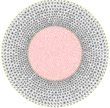
1.2 The chosen model problem for chapter 2 . . . 11
1.3 One possible empirical optimization algorithm: the surface method . . . 12
1.4 Solid line: Graphical representation of the solution manifold M. Dotted line: A possible trial space . . . 14
1.5 One way of constructing a reduced basis: the Frechet differentiable case . . . 16
1.6 Localized Reduced Basis . . . 21
1.7 Solid line: truth solution; Dotted line: Best projection onto some reduced basis; Dashed line: Output of a system with no proper stabilization . . . 29
1.8 Trajectories for the finite dimensional model problem . . . 34
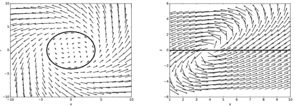
1.9 Analysis of the model problem. Left: projection onto the x ≠ y plane. Right: projection onto the x ≠ z plane . . . . 34
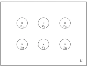
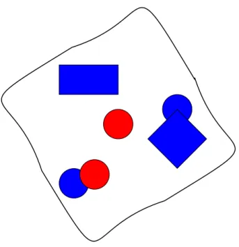
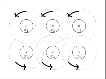
2.1 The chosen model problem. Here, Nobs= 6 . . . 42
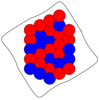
2.2 An illustration of the concept of solution partitioning . . . 42
2.3 The original Schwarz problem . . . 43
2.4 As possible reference mesh ˆΩ . . . 45
2.5 Method developed in [131] . . . 46
2.6 The chosen reference mesh. In red: ˆΩint; in black: ˆΩtampon . . . 47
2.7 F◊(ˆΩ), for various values of ◊ . . . . 47
2.8 Three snapshots taken from M . . . 48
2.9 Three snapshots mapped back onto the reference domain . . . 48
2.10 Possible generic subdomains ˆΩj . . . 50
2.11 First application of ORBEM: a sparse collection of interesting subdomains . . . . 50
2.12 Second application of ORBEM: a dense collection of subdomains, following a pattern 51 2.13 The ORBEM method allows for the rotation of the local basis . . . 60
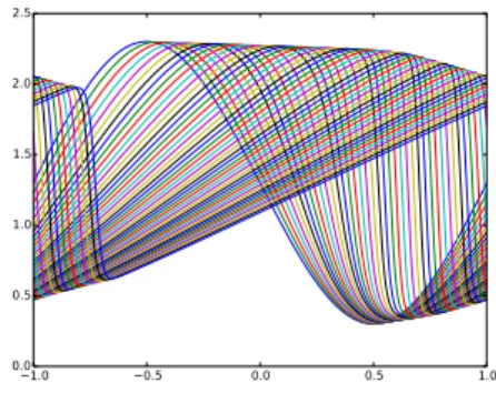
3.1 Snapshots of the solution to the unsteady viscous Burger equation with u0 = ⁄ + sin(x), ⁄ = 1.3, ‹ = 4, ‘ = 0.04 . . . . 73
3.2 Calibrated set of the above snapshots for u0= ⁄ + sin(x), ‹ = 4, ‘ = 0.04 . . . . 74
3.3 Eigenvalues of the POD decomposition of the original set of snapshots ( in red) and of the calibrated set of snapshots (in green) . . . 74
3.4 3rd (left) and 6th (right) POD modes for the calibrated (green) and original (red)
simulations . . . 75
3.5 intro items . . . 75
3.6 A few values of the quantities (3.57) as a function of ∆“. The x axis is scaled to multiples of c ú ∆t. . . . 78
3.7 A few values of the quantities (3.57) as a function of ∆“. The x axis is scaled to multiples of c ú ∆t. . . . 79
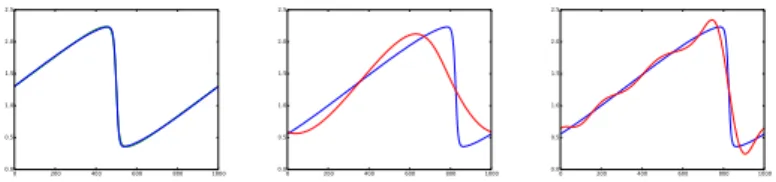
3.8 Relative L2-error of the solution as a function of time for different values of the reduced basis. The three curves close to the x-axis (almost overlapping at this scale) are the associated best approximation errors. . . 79
3.9 Relative L2 best projection errors, on the training set . . . . 80
3.10 Relative L2 error of the reduced solutions, on the training set . . . . 81
3.11 This method requires an overlapping decomposition of Ω . . . 82
3.12 Snapshot sets at different steps of the offline stage. From left to right: snapshots with no calibration; centered snapshots; truncated snapshots . . . 85
3.13 The indicator function, that depends strongly on the solution manifold at hand . 85 3.14 Snapshots in the resulting "coarse" solution manifold M0 . . . 86
3.15 Top left : projection of one snapshot, with no calibration, on a basis of cardinality 15; Top right : projection of the truncated snapshot onto an adapted basis; Bottom : projection of the complement on a small Fourier basis . . . 86
3.16 On possible ouput of an offline calibration procedure such as algorithm 5 . . . 90
3.17 The output of the hierarchical clustering algorithm, for the snapshot set presented Figure 3.16 . . . 91
3.18 Snapshots for various times, and various convection parameters c(µ) . . . . 94
3.19 Reference mesh . . . 94
3.20 Meshes on which the physical solutions un= ˆun ¶ Fn are defined . . . . 95
3.21 Fine mesh on which the offline stage is performed . . . 96
3.22 Left: A snapshot near the beginning of the simulation; Right: a snapshot near the end of the simulation . . . 97
3.23 The truncated mesh . . . 97
3.24 Truncated versions of the solutions presented in Figure 3.22 . . . 98
3.25 caption . . . 99
3.26 Green: the ’true’ inflow direction; Blue: the guessed angle . . . 101
4.1 Position of the shock for various AoA and Mach numbers. Coloured lines: Barycen-ters of the cells in which the shock is located; Black lines: Fitted line through these barycenters . . . 106
4.2 The solutions of the problem for AoA={0.0¶, 1.0¶, 2.0¶, 3.0¶} and Mach={0.81, 0.82, 0.83 } . . . 110
4.3 The x velocity component at the wing in the uncalibrated case : a few POD basis 110 4.4 1st, 3th and 5th POD basis at the wing in the uncalibrated case for the full domain Ω111 4.5 Physical domain Ω . . . 112
4.6 The reference domain ˆΩ, and one possible instance Ω(µ) := F≠1 µ (ˆΩ) . . . 113
4.7 The x velocity component at the wing in the calibrated case : a few POD basis . 115 4.8 1st, 3th and 5th POD basis in the calibrated case for the left subdomain . . . 116
4.9 Truth solution for velocity component with Mach=0.81 and AoA=3.0¶ . . . 125
4.10 The identity mapping velocity component on a flat domain . . . 125
List of Figures
4.12 Reference domain ˆΩ . . . 127
4.13 Physical domain Ω . . . 127
4.14 Left: fi3 in the original formulation, with homogeneous Neumann boundary con-dition; Right: fi3 for a more suitable boundary condition . . . 128
4.15 Modification of weights and projection functions to get smoother transitions on ˆΓ1 and ˆΓ3 . . . 129
4.16 The mapped solution for velocity component on a curved domain . . . 130
4.17 One of the entries of the Jacobian matrix, namely (JF≠1 n )11. Left: with no addi-tional smoothing ingredients; Right: with some smoothing ingredients . . . 131
4.18 Comparison of the outputs . . . 132
5.1 We restrict ourselves to solutions with at most one shock . . . 139
5.2 Away from the shock, the foot of the characteristics are close . . . 140
5.3 Size of- --Zµ +”µ t,0 ≠ Zt,µ0 -- . . . 141
5.4 Ω ◊ [0, T ] ◊ Uadin the non calibrated case . . . 143
5.5 Solving for p(x, 0) . . . 145
5.6 Ω ◊ [0, T ] ◊ Uadin the calibrated case . . . 147
5.7 Characteristics in the calibrated case . . . 148
6.1 Divide and conquer . . . 160
7.1 Non linear operator acting on the solution manifold . . . 168
Avant-Propos
Avant-Propos
Cette thèse s’est effectuée au laboratoire Jacques Louis Lions (LJLL), à l’Université Pierre et Marie Curie (UPMC). Elle a été financée dans le cadre du project MECASIF, dont l’objectif était de rapprocher industriels et universitaires sur des problèmatiques de réduction de modèles. La thèse devait répondre à un problème soulevé par Bertin Technologies et s’est faite sous la direction d’Yvon MADAY.
Préambule
Le chapitre introductif commence par une description du problème cible, l’objectif que nous nous sommes fixé en début de thèse. Après avoir décrit brièvement une méthode type, empirique, utilisée aujourd’hui pour résoudre ce problème cible, nous motivons le besoin pour une approche plus rigoureuse, qui tienne compte de la très grande complexité du problème due aux nombreuses échelles spatiales impliquées. Dans cette direction, nous décrivons la méthode de bases réduites, qui répond simultanément aux deux contraintes: un cadre théorique rigoureux ainsi que des coûts de calculs réduits. La fin du chapitre introductif insiste sur le fait que certaines questions liées à l’application de méthodes type «bases réduites» au problème cible n’ont pas encore été résolues. C’est à quelques unes de ces questions que nous tentons de répondre dans les autres chapitres.
Dans le chapitre 2, nous étudions la facette «variabilité géometrique» du problème cible, et nous le faisons indépendamment des autres difficultés soulevées dans le chapitre introductif. Il apparait assez clair que cette problématique est proche des méthodes de décomposition de domaine, et que notre méthode devra être adaptée au contexte qui est celui de la réduction de modèles. Après avoir rappelé les quelques approches de la littérature proches de nos besoins, nous concluons sur la nécessité du développement d’une nouvelle méthode, plus flexible et proposons un cahier des charges. Le reste du chapitre est consacré à la description et à l’analyse d’une méthode répondant aux besoins fixés.
Dans le chapitre 3, nous cherchons de nouveaux outils à ajouter à la réduction de modèles standard et qui permettent de traiter des problèmes pour lesquels les variétés solutions ont une grande épaisseur de Kolmogorov. Nous commençons par décrire la méthode de Freezing, disponible dans la litterature et qui est une réponse possible, mais pas entièrement satisfaisante à la problématique du chapitre. Le reste du chapitre est consacré à la description d’une méthode alternative, la calibration. Des tests numériques sur l’équation de Burgers visqueux dans le cas périodique, viennent confirmer la viabilité de l’approche.
Dans le chapitre 4, nous appliquons la méthode de calibration à un problème plus réaliste: un écoulement autour d’un profil NACA. L’application de la calibration à ce problème qui est un problème en dimension deux, hyperbolique, et non périodique, pose de nouvelles difficultés que nous tentons de résoudre. De nombreux ingrédients sont nécessaires pour la résolution complète de ce problème. Par conséquent, la section numérique se concentre sur quelques aspects, ceux qui nous paraissent les plus importants.
La calibration dans les chapitres 3 et 4 est utilisée pour réduire l’épaisseur de Kolmogorov de variétés solutions. Le chapitre 5 part du constat que la calibration amène une propriété supplémentaire: elle ajoute à la régularité des solutions, comme fonction des paramètres. Ceci est vrai quelque soit le problème étudié. Un exemple particulièrement parlant, et celui que nous
avons choisi de traiter dans ce chapitre, est celui de problèmes hyperboliques, avec une forte dépendence de la position du choc aux paramètres. Nous décrivons quelques idées préliminaires vers le calcul des dérivées des solutions par rapport aux paramètres, une première étape vers la résolution de problèmes de control optimal dans ce contexte.
Les deux derniers petits chapitres de cette thèse sont un peu à part, mais sont le résultats de réflexions connexes à celles des chapitres principaux. Pour le calcul de la décomposition en modes propres orthogonaux pour des problèmes instationnaires et/ou des espaces de paramètres qui ne sont pas de toute petite dimension, il est intuitif de vouloir utiliser une méthode «diviser pour régner». C’est à la question de l’erreur due à une telle approche que nous tentons de répondre dans le chapitre 6.
Le point de départ du chapitre 7 est le constat que les méthodes inspirées par le big data ren-contrent un intérêt croissant dans la communauté «bases réduites». Nous mentionnons quelques travaux récents et prometteurs dans cette direction. Nous nous arrêtons ensuite plus longuement sur la méthode DMD ( Decomposition en Modes Dynamiques ) et utilisons son analyse pour met-tre en garde sur le fait qu’il existe des situations dans lesquelles une phase d’apprentissage «force brute» ne remplace pas une bonne modélisation, et ce quelle que soit la quantité de données assimilées.
Preamble
1
The introductive chapter starts with a description of the target problem, the initial goal of the thesis. After briefly discussing existing empirical models, we motivate the need for an approach with a stronger theoretical background: we choose to use reduced order modeling. We give a quick overview of how ROM is usually performed, and insist on the properties a problem should satisfy in order to be a good ROM candidate. We then provide evidences showing that the target problem is not, at first glance, suitable for ROM, and that additional steps need to be performed. In chapter 2, we study difficulties due to the geometry variability of the target problem. We work with a model problem, that helps isolating this one issue from the other mentioned in the introductive chapter. We then give a quick overview of the ROM methods available in the literature that are designed to handle geometry variations. We show that there is a need for a method more flexible than the existing ones. The remainder of the chapter is devoted to the development of such a method.
In chapter 3, we try to develop a method that allows for the use of ROM in the context of solution manifolds with large Kolmogorov n-widths. We describe the method of Freezing that is a interesting answer to this specific problem, but not entirely satisfactory in our opinion. The remainder of the chapter focuses on the description of an alternative method: the so-called calibration. Numerical experiments are performed on the periodic viscous Burgers equation, and tend to confirm the viability of the method.
In chapter 4, we apply the calibration method to a more realistic problem: the flow around a NACA airfoil. This leads to additional challenges, as the solutions present shocks, whose positions are strongly parameter dependent. Also, the domain is now two dimensional, and we are not in the favorable periodic setting. A complete numerical scheme is quite involved, and we have rather chosen to focus on a reduced number of issues, the ones we consider the most important.
The calibration is used in chapter 3 and 4 to diminish the Kolmogorov n-width of solution manifolds. Chapter 5 starts by noticing that calibration adds a bonus property: it improves the regularity of the dependency of the solutions with respect to the parameters. This is true whatever the problem studied. An especially enlightening example, and the one we have chosen to study in this chapter, is the one of hyperbolic problems, where the shock positions’ sensitivity to parameter variations is high. We end the chapter by deriving a few preliminary results, towards the development of numerical schemes for the computation of parameter derivatives of the solutions.
1
The last two small chapters of this manuscript are a little different, but discuss connected topics. For the computation of proper orthogonal modes for time dependent problems and/or for parameter spaces with moderate dimensions, it is natural to apply a divide and conquer strategy. Chapter 6 gives bounds on the errors due to this kind of approach.
The starting point of chapter 7 was to notice that big data related ideas were receiving more and more attention in the reduced basis community. We start by mentioning some recent and promising results in that direction. We then discuss the DMD ( Dynamic Mode Decomposition ) method, and use its analysis to warn for inconsiderate use of such approaches. There are some cases, where brute force can not replace a good model, whatever the amount of data assimilated.
Chapter 1
Introduction
This first chapter is an extended introductory chapter. We start with a short description of the target problem, the original objective of this thesis. After briefly discussing existing empirical models, we motivate the need for an approach with a stronger theoretical back-ground: we choose to use reduced order modeling. We give a quick overview on how ROM is usually performed, and insist on the properties a problem should satisfy in order to be a good ROM candidate. We then provide evidences showing that the target problem is not, at first glance, suitable for ROM, and that additional steps need to be performed. We finally detail how each of the chapters of this thesis is a new step towards the objective.
The first section states the starting point of the thesis. We briefly discuss the context in which this study takes place. The introductory section ends with a motivation for the use of Reduced Order Modeling (ROM). We then give an overview of the ROM framework. Instead of a general, heavy presentation, we have chosen to illustrate it on a simple heat equation. The end of this chapter is devoted to showing that there were (and still are) many ingredients missing to provide a complete ROM based solution to solve the initial objective. Following this remark, we have focused on simpler, more reasonable objectives. Some of them will seem far away from the initial goal. we consider them as steps, or elementary bricks, towards a sensible and robust solution to the initial objective.
1.1 Vertical axis wind turbine placement optimization
Wind farms have started catching attention for clean energy production for a few decades now. To get a grasp of their growing importance, one can for instance take a peak into the list of major European offshore wind farms, in [103]. The infatuations of the beginning have opened up to a more mature market where optimization of cost, production and maintenance hold a bigger place.
Whatever the precise objective function, these optimization problems have many layers of complexity. Indeed, for such problems, many length scales are involved, each having interacting influences. The scales identified a priori are: the scale of the boundary layer, the scale of the wing (shape, material etc.), the scale of the farm (for instance, the relative placement of the turbines), and finally the atmospheric scale (required for boundary conditions). The first two scales have already received some attention because of the many different applications among which aeronautics. It also benefits the fact that experiments in wind tunnels can easily be
programmed and conducted. The last two scales are more difficult to study, from a theoretical stand point as well as numerically and experimentally.
In this thesis, the focus has been put on optimization at the scale of the farm. The analysis of the measurements of working wind farms have shown that the average power loss due to the influence of upstream turbines averages 10% to 20%. It is also shown that in the wake, one finds higher level of turbulence, and thus higher loads on the turbines, which means higher maintenance costs. Many different configurations have been and are currently being tested. We mention two of them: in [15], the authors describe a bow shaped windfarm. A more natural ’grid’ type farm is studied in [56]. The question that has naturally risen is: is there a way to diminish the wake effect as well as the load imposed on the turbines by adjusting the placement of the turbines ?
The (very ambitious) objective of the thesis was to give an optimized wind farm layout given the shape (or model) of a turbine, some constraints on the positioning of turbines and some other physical parameters (such as boundary and initial conditions). We have restricted the study to offshore windfarms and vertical wind turbines. This provides with useful assumptions: we do not have to take into account the topography. Also, vertical wind turbines allow for the use of a cylindrical symmetry. The turbines are not sensible to the inflow direction, and the only parameters for a given turbine shape are the direction and speed of rotation.
We note right away that even if the optimization only takes place at the scale of the farm, the behavior at other scales aforementioned still need to be modeled. In other words, the computation for one specific configuration is already a challenging task. But the situation is even worse: the objective being optimization, we are in a many-query context. This means that a focus needs to be put on the computational cost of the method.
The majority of the literature on the computation of the power output of wind farms uses rough empirical models1. We start our journey by giving a very quick overview on how these
models are constructed, and on the theoretical results they rely on. We then give the major draw-backs of these approaches. This serves as a justification for the central discussion of this thesis: how to use the theory of Partial Differential Equations (PDE) and Reduced Order Modeling (ROM) to solve the optimization problem at hand.
A complete state of the art of the engineering methods currently being used to estimate a priori the output of a wind turbine farm is out of the scope of this thesis. We refer to [38, 55] for surveys, and have rather chosen to briefly present one ’generic engineering method’. We underline some of its flaws and thus motivate the need for more advanced models. We also take this opportunity to once again highlight the overall complexity of the task at hand.
The first component, common to all rough engineering models, is a wake deficit to power output relation. We describe one possible route. Let some cylindrical control volume around the rotor, with the longitudinal axis in the direction of the flow. The process is illustrated in Figure 1.1. We apply the conservation of momentum equation and suppose that the viscous term, the pressure term, basically all terms except the convective term and the force due to the turbine are negligible. Some hypotheses can be justified by physical considerations and we refer to the aforementioned articles for more details. We denote with u the velocity, with T a source term that represents the force acting on the turbine, with fl the density and with Ê the cylindrical control volume of interest. We end up with a relation such as:
⁄
ÊÒ · (flu ¢ u) ¥ T.
Denote uinand uout respectively the inflow and the outflow. We apply the divergence theorem
1
1.2. PDE models
uin uout
Cylinder w Turbine
Figure 1.1: One possible starting point for engineering models
and assume rotational invariance. Let ˆÊsecbe one section of Ê. At first order in uin≠ uout, we
have: ⁄
ˆÊsec
fluout(uin
≠ uout) ¥ T. (1.1)
We can see how, by placing such models end to end, one can derive a first naive way of estimating the power output of wind farms with aligned turbines.
To get more advanced models and results for more general configurations, one needs to add other components to try and account for other various physical phenomenon. We mention a few of them, but there are as many variants as there are paper on the topic. For instance, one needs to model the wake geometry, or equivalently a procedure to select the downstream turbines that are being impacted by a given wake. In [82] they try using a reasoning similar to the one that lead to equation (1.1) to account for the interaction between wakes. Other models have been constructed to estimate the power loss due to an increase in the turbulence intensities, see for instance [15]. This type of rough modeling is currently being used on real life data. The numerical results presented in the literature often compare the energy output of the model with experimental data. Thanks to the extra degrees of freedom given by parameters in the model, a reasonable match is (most of the time) found between the two.
The examples of more advanced modeling just mentioned illustrate something important: there are many effects that need to be taken into account. The propagation of the wake, the wake interactions, and the change in the nature of the flow (increasing turbulence levels) have important effects on the output. One can not conclude, a priori, on the effects that can be ne-glected. For instance, a model that accounts for wake interaction, without discussing turbulence levels may be dubious.
I draw two important conclusions from this short analysis. The first one is that there is a need for more advanced modeling, to better understand the different mechanisms and their influences. The second conclusion is that it will be hard to find intermediate steps between the rough calculations resulting in relations such as in (1.1), and the full solution of the problem. The objective of this thesis is to find such steps (that might look like sideway steps) towards a complete resolution of the problem, or at least towards a model with rigorously justified assumptions.
1.2 PDE models
As a more realistic approach, we have chosen to use the theory of Partial Differential Equations (PDE). We take advantage of this section to define some notations that will be used throughout
this manuscript. Ω denotes a smooth domain in Rd where d œ 1, 2, 3. The problems considered
will often be time dependent PDEs and the model equation that we have chosen to work with is:
’t œ [0, T ], ˆuˆt + L(u) = f on Ω. (1.2)
To complete the system, and have a chance to have a well posed problem, one needs to provide appropriate initial u(t = 0) = u0 and boundary conditions for u or ˆnˆu on ˆΩ. L will be
throughout this manuscript a first or second order partial differential operator.
We make a constant use of the following functional spaces: L2(Ω) the space of square
in-tegrable functions over Ω; H1(Ω) := Óuœ L2(Ω), Òu œ!L2(Ω)"dÔ. Also, denote H1
0(Ω), the
elements of H1(Ω) with zero trace. That is H1 0(Ω) :=
)
uœ H1(Ω), and u = 0 a.e on ˆΩ*.
Let Y be any real Hilbert space. We will denote by < ·, · >Y and Î · ÎY := Ô< ·, · >Y the
scalar product and the norm respectively. The dual space of Y will be denoted YÕ. For instance,
!
H1 0
"Õ(Ω) = H≠1(Ω). For an introduction on Sobolev spaces, we refer to the reference book on
the subject [4].
In this thesis, our focus will be put mainly on three equations. A rigorous theoretical presen-tation of each of them is not in the scope of this thesis, nor is it its topic. We briefly state here some of their characteristics, and detail the chapters of the thesis and the particular contexts in which each of them appears.
Burgers We will encounter in this manuscript both the viscous ‘ > 0 and inviscid cases ‘ = 0. The viscous case is a one dimensional non linear but simplified model of the Navier-Stokes equations. It allows for simple numerical experiments, as will be conducted in chapter 3. The inviscid case is a simple hyperbolic problem, and is often chosen as a first test case for hyperbolic solvers in the literature. We will throughout this manuscript focus on the viscosity, physically meaningful solutions. We will use it in chapter 5 as a model for Euler equation.
Euler We will study this equation in a two dimensional setting in chapters 4 and 5. It is, as the inviscid Burgers equation, an hyperbolic problem. Our main focus will be put on the development of shocks.
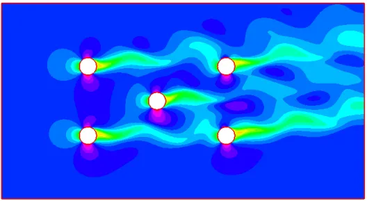
Navier-Stokes This is the target equation. Because of the issues that will be raised in section 1.5, we will actually not work with it a lot in this manuscript. We present in Figure 1.2 the model problem we work with in chapter 2. The wind turbines are modeled by cylinders, to focus on the optimization of the geometry of the farm, rather than on the realistic computation of a CFD flow around a turbine. Navier-Stokes simulations are also performed in the numerical experiments of section 3.9.
1.2.1 Numerical methods
A discussion about the (many) different numerical schemes used for CFD computations is not in the scope of this manuscript. This is the topic of many books in the literature, for instance [8] or the more recent [34]. Also, a more specific overview of PDE solvers’ specificities for the computation of flows around wind turbines can be found in [134]. We only briefly come back one aspect. Instead of considering realistic physical blade bodies, one can model the wind turbines with equivalent source terms. The most commonly used methods in that direction are the actuator disk and actuator line models. A presentation of both methods can be found in [97]. The form of the source term is chosen using basic physical considerations in the same
1.2. PDE models
Figure 1.2: The chosen model problem for chapter 2
vein as the ones that were used in section 1.1. The numerical results obtained for wind farm flow computations are promising. But as for the engineering models, they require parameter fitting. More precisely, one has to tweak the parameters of the modeled blade for each numerical simulation. One can argue that the quality of the results presented is mitigated by this parameter fitting. Nevertheless, this method can be seen as an intermediate method between the complete numerical solution, and the basic engineering models such as the one presented in section 1.1.
This type of methods will not be further studied in this manuscript, and this for a very simple reason: we use even coarser approximations in the course of this thesis. In chapter 2, we use cylinders to model the windturbines. The chapters that follow use simpler shapes or even different equations, to focus on very specific issues.
We conclude this short section by stating one important assumption, that we will have to keep in mind all through this manuscript. It actually explains why we do not further discuss the standard numerical CFD methods. We assume that we have a fine solver that exactly captures the true physical solution. This fine solver can for instance be of Finite Elements (FE) type, of Finite Volumes (FV) type or a Discontinuous Galerkin (DG) scheme. To insist on the fact that the resulting solution cannot be distinguished from the continuous solution, it is often referred to as ’truth approximation’. The reasons for this point of view is easily understandable. Behavior/structures that can not be captured by fine schemes, are out of reach of the desired cheap approximate solvers. The best thing the latter can do is try and match the ’best known’ solutions, which are the ones obtained with fine schemes.
Remark 1 Only a few references do not use this premise. In [93, 127], the idea is to use data
possible, we allow for a bias in the model.
We denote from now on N the number of degrees of freedom of the chosen fine solver providing the truth solution. This gives us a reference computational cost. More precisely, any computational cost of order N will be considered a high cost.
1.3 A first try at optimization
Figure 1.3: One possible empirical optimization algorithm: the surface method
We present one more method before entering the core of this manuscript. It is intermediate between the engineering models of section 1.1 and the full reduced model framework of the remainder of this thesis. Let D be a parameter space and let J be a functional defined on D that we are trying to minimize. What we describe is a typical surface type method, an empirical answer to parametrized problems that can be easily implemented. We present a possible implementation in Algorithm 1 below.
Data: Parameter space: D Result: µopt
Define Ξ0 some coarse sampling of the parameter space;
Compute the solution u(µ) for each µ œ Ξ0; repeat
Find Êkµ D such that J(µ) is small for µ œ Ξkfl Êk ;
Sample more finely D in wk: Ξk+1;
Compute the solution u(µ) for each µ œ Ξk+1;
kΩ k + 1 ;
untilsome accuracy/computational cost condition;
Algorithm 1: Surface type method
An illustration of this algorithm for a parameter space embedded into R2is shown in Figure
1.3. The blue dots represent parameters for which the truth solution has been computed. This method requires the estimation of J in between sampled points. This is achieved using an interpolation procedure. The latter is an important component of the method and has a big impact on the overall accuracy. But as there is no theoretical results associated, it is done
1.4. Model order reduction empirically. The direct consequence is that in order to achieve a decent accuracy, one needs to perform many fine scheme computations. It is obvious that this is not in accordance with the goal of computational cost reduction. Moreover, this issue is made even worse because of the curse of dimensionality. Indeed, as the parameter space is a subspace Rdim(D), for a fixed
discretization step in the parameter space (and so equivalently for a fixed accuracy) the number of fine computations required grows exponentially with dimension of the parameter space. The model order reduction framework gives a theoretically more sound and computationally more reasonable answer to this kind of parametrized problem.
1.4 Model order reduction
We start with a macroscopic overview of the framework as well as its main requirements. We then detail the steps and key results. For a more thorough presentation, we refer to the two recent books on the subject, [68] and [109]. We denote from now on with µ a generic parameter and with D a generic parameter space.
The objective is to construct a method that allows for many queries of the type µ æ u(µ). Let µ œ D. The solutions u(µ) are typically solutions to some PDE:
Y _ _ ] _ _ [ ˆu(·,t;µ) ˆt + L(u(·, t; µ)) = f in Ω u(µ)(t = 0) = u0 in Ω u or ˆu ˆn = g on ˆΩ. (1.3)
ROM assumes no a priori parametric dependence. f, u0, g, Ω and L may depend on the parameter
µ. We will always explicitly state the parametric dependency. The question that model order
reduction tries to answer is: is there some regularity, whatever the precise meaning, of ; D æ X
µ ‘æ u(µ) (1.4)
and if so, can we take advantage of it to accelerate the computation of (1.4). Our motivation in this manuscript is optimization. Note that this can also be used to solve inverse problems. In the course of this thesis, the regularity of (1.4) will take various forms. It ranges from differentiable with an explicit derivative, as in section 1.4.1, to cases that require a preconditioning step, see section 1.5.1.
The fundamental notion for ROM that will be used throughout this manuscript, is the concept of solution manifold. Several definitions are possible depending on the context, see for instance the introduction of chapter 3. The most common one2, that will be used unless specified, is given
by:
M := {u(·, t; µ), µ œ D, t œ [0, T ]} . (1.5)
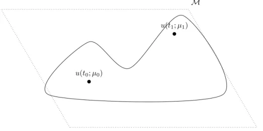
The name manifold is not chosen loosely. The premise of ROM is to think of M as a smooth manifold, embedded in a well chosen Hilbert space X, even if no theoretical results regarding regularity are available for most real life problems.
As we are aiming for the reduction of the computational cost of solutions in M, one sensible first step is to try to capture and compress the characteristics of this manifold. One adapted
2
One sometimes considers a space time formulation, which results in a different solution manifold, see for instance [20].
M
u(t0; µ0)
u(t1; µ1)
Figure 1.4: Solid line: Graphical representation of the solution manifold M. Dotted line: A possible trial space
theoretical tool is the notion of Kolmogorov n-width. This quantity measures the ’linear width’ of any subset of normed spaces. More precisely, for any manifold M it is defined as:
dn(M, X) := inf En sup fœM inf gœEnÎf ≠ gÎ X. (1.6)
The first infimum is taken over all linear spaces of dimension n embedded in X. A graphical example is presented in Figure 1.4. The Kolmogorov n-width returns the worst approximation, on the best linear space of dimension n. A few theoretical results are available to estimate a priori this n-width. In [99], they prove n-width estimates for solutions to elliptic problems where the parameter dependence is on the source term. The latter is taken in some compact of a high order Sobolev space. A more recent result gives estimates of the Kolmogorov n-width under holomorphic mappings [35]. More precisely, they show that the exponential decay of the n-width is conserved through the image of a Frechet differentiable function.
We conclude this overview of ROM by introducing the offline/online paradigm. The capture and modeling of the characteristics of the solution manifold M can be seen as a learning phase, referred to as offline in the ROM community3. It often amounts to creating a linear space of
moderate dimension, that represents well M. The target error, for a fixed basis size, is given by the Kolmogorov n-width. This learning phase is expensive from a computational cost, as it involves the computation of a moderate number of fine solutions. The online phase uses this learning phase, and provides a way of computing approximations of members of M at a reduced cost4. The analytical example of the next section will help understand this concept of
offline/online stages.
3
A tabular expliciting other similarities between ROM and machine learning algorithms is presented in chapter 7.
4
1.4. Model order reduction
1.4.1 Analytical example
As stated in the preamble, we have chosen to tackle the description of ROM by focusing on toy examples. The first one we study is a favorable case, as the regularity of the problem with respect to the parameter is explicit. Let the following heat equation:
; ≠Ò · (µÒu) = f in Ω
u = 0 on ˆΩ. (1.7)
We choose a parameter space D that satisfies: I
D is a compact subspace of LŒ(Ω)
÷µminœ R+ú, ’µ œ D, µ > µmin a.e in Ω.
How do the solutions u(µ) behave when we change the diffusion coefficients ? Existence and uniqueness of the solution in H1(Ω) are guaranteed by classic Lax-Milgram theory for coercive
and continuous operators.
We study the limit of u(µ + h‹) ≠ u(µ) for a fixed direction ‹ contained in the unit ball of tangent space of D and h œ R. Let uh:= u(µ + h‹) and let vh:= uh≠ u(µ). Using the linearity
of the equation, the latter is solution of:
; ≠Ò · (µÒvh) = ≠hÒ · (‹Òuh) in Ω
vh = 0 on ˆΩ.
We can compute the standard a priori estimates for vh. For this, multiply the first equation by
vh and integrate by parts:
⁄ Ω µÒvh · Òvh= h ⁄ Ω ‹Òuh Òvh.
We have used vh zero on ˆΩ. We use the hypotheses on D and on ΋Î
LΠto show the a priori estimate:
µmin|vh|H1 Æ h|uh|H1. To conclude, we use the a priori estimates on uh:
µmin|uh|2H1 Æ ÎfÎH≠1ÎuhÎH1, with the Poincare inequality:
÷C œ R, s.t µmin|uh|H1 Æ CÎfÎH≠1, to finally obtain the following a priori estimates on vh:
|vh |H1 Æ 1 µ2 min ChÎfÎH≠1. (1.8) Let w(µ, ‹) œ H1 0(Ω) be the solution to ; ≠Ò · (µÒw) = ≠Ò · (‹Òu(µ)) in Ω w = 0 on ˆΩ.
To prove Gateaux differentiability, we will prove estimates on:
÷ :; D, D, R æ H
1(Ω)
We know:
≠Ò · (µÒ÷(µ, ‹, h)) = ≠Ò · (µÒ (u(µ) ≠ u(µ + h‹) ≠ hw(µ, ‹)) = Ò · ((h‹)u(µ + h‹)) + hÒ · (µw(µ, ‹)) = Ò · ((h‹)u(µ + h‹)) + hÒ · (‹u(µ)) = Ò · ((h‹)Ò(u(µ + h‹) ≠ u(µ)). This gives a priori estimates on ÷:
µmin|÷(µ, ‹, h)|2H1Æ h|÷(µ, ‹, h)|H1|u(µ + h‹) ≠ u(µ)|2H1. We use the estimates on vh= u(µ + h‹) ≠ u(µ), see equation (1.8), and obtain:
µmin|÷(µ, ‹, h)|H1 Æ 1
µ2
min
Ch2ÎfÎH≠1. (1.9)
This concludes on the Gateaux differentiability of the application, in the direction ‹, with deriva-tive w(µ, ‹). Moreover, since for all µ œ D,
w(µ,·) :; D æ H
1 0
‹ ‘æ w(µ, ‹)
is linear and continuous, we conclude on the Frechet differentiability of the parametrized problem over D.
From this analysis, we have one natural way of developing a method to approximate µ æ u(µ) at reduced cost. The first step is construct a good representation of the solution manifold M. The Frechet differentiability provides an easy solution, that we illustrate in Figure 1.5. Define
M
u(µ0)
u(µ1)
Figure 1.5: One way of constructing a reduced basis: the Frechet differentiable case some threshold ‘, the maximum approximation error that we want on our solution manifold M. Sample the parameter space such that:
’µ œ D, ÷µiœ D, s.t Îu(µ) ≠ u(µi) ≠ wµi(µ ≠ µi)ÎH1Æ ‘.
The a priori estimates on ÷, see equation (1.9), allow us to compute a rigorous distribution of {µi}iand the corresponding Frechet derivatives {wµi}i. This ends the offline phase as introduced
1.4. Model order reduction in the previous section. The online phase is even easier in this setting. For any µ œ D, we just have to pick µ0in the pre computed set the closest to µ. We then have an explicit formula for an
approximation of u(µ). The guaranteed error estimate is the chosen threshold ‘. Because of the Frechet differentiability, independent of the direction, we feel that we are starting to overcome the curse of dimensionality.
We note the main differences with a realistic case. First of all, the smoothness with respect to the parameter does not often translate into an explicit formulation. Sometimes, the manifold even needs some preconditioning to enforce smoothness, see for instance chapter 5. Also, it feels like this type of construction neglects a lot of redundancy. For instance, we expect redundant pieces of information to be found in solutions for parameters far away in the parameter space. Nevertheless, the methodology developed on this analytic example is exactly the same as what is being done for ROM for real life problems, and is enlightening in that respect. The next section describes a typical offline phase.
1.4.2 ROM, the offline phase
As already stated, the first necessary step is to construct a basis that captures most of M. More precisely, we are looking for Ψ, a set of N functions in X the underlying Hilbert space, such that:
’u œ M, ÷uN
œ span Ψ, Îu ≠ uN
ÎX small .
This first necessary step is the sampling of the parameter space. That is, we need to choose a representative set:
Ξ:= {µk, k = [1 . . . N ]} µ D.
It is easy to see that the size of Ξ influences the offline computational cost as well as the online accuracy of the method. The selection of the set Ξ is almost always 5 done empirically. The
reduced basis is then picked as a subspace of:
span {u(µk), µk œ Ξ} µ X.
The way the compression of the information contained in {u(µ), µ œ Ξ} is done, varies among the many methods available. We mention here a few of them, the ones we feel the closest to our objective. A geometric approach close to the Centroidal Voronoi Tesselation (CVT) has been developed in [46, 25]. The parameter space is splitted using a CVT algorithm. In solid mechanics, the most commonly used algorithm is the Proper Generalized Decomposition (PGD) [83]. This greedy approach results in a separable approximation of the solution, along the different dimensions: time, space and parameter for instance. It is empirical for most applications. We mention some of the theoretical results are available. If the problem actually is a separable problem, then the PGD algorithm reduces to a POD algorithm (that we will detail below), see [102]. Also, for the Poisson equation in the 2 dimensional unit square, it can be shown that each greedy iteration is well posed, and that the algorithm converges, see [85]. Finally, we mention the Balanced Truncation method [118], which is built on a ’Linear Time Invariant’ form of the system to solve.
We now give more details on the two methods that will be used in the rest of the manuscript. They are dominating in the ROM community, especially for CFD computations. We underline the up and downsides of both methods and conclude on the purposes they should be used for.
5
1.4.2.1 Reduced Basis (RB)
In this section, we give an overview of the reduced basis method. It relies heavily on the existence of a cheap, rigorous error estimator. That is, for each reduced basis Ψ := {Âi}, it requires an
application:
∆Ψ:; D æ R
µ ‘æ ∆Ψ(µ),
that is an upper bound on the actual error made on the reduced basis approximation. More precisely, for u(µ) the truth approximation and uN(µ) the reduced basis Galerkin approximation,
it should satisfy:
’µ œ D, Îu(µ) ≠ uN(µ)ÎX Æ ∆Ψ(µ).
The construction of such an error estimator is described in chapter 3. The greedy algorithm follows naturally:
Data: Fine sampling of the parameter spaceD: Ξ
Threshold ‘
Maximum size of the basis Nmax
Result: Reduced basis Ψú
kΩ 0;
µ0Ω random parameter in D;
Ψ0:= {u(µ0)};
while k < Nmax and ∆
Âk > ‘ do µk+1:= argsup µ ∆Ψ k(µ); Ψk+1:= Ψkfi u(µk+1); kΩ k + 1; end Ψú:= Ψk;
Algorithm 2: The greedy RB method
Recent results [23] show that if the Kolmogorov n-width of the solution manifold M decays exponentially, i.e if:
÷c, C œ R2 s.t ’n d
n(M, X) Æ ce≠Ck, (1.10)
then the basis obtained using the greedy algorithm described above inherits this property: ÷(cÕ, CÕ) œ R2, depending on (c, C) s.t ’N, supuœMinfuNœΨN . .u≠ uN.. X Æ c Õe≠CÕ N (1.11)
Similar results are available if the argsup during the greedy algorithm is not done exactly [43]. This method’s main advantage is obviously its computational cost. Indeed, only a moderate number fine computations need to be performed, thanks to the error estimator. Another inter-esting property is that we have a guaranteed error bound on a fine sample of D. The major downside is that that for non linear problems, the error estimators available are not reliable, as the bounds are not tight. This reduces a lot the range of application of this method. It will be discussed in section 1.4.3.1 where we explain how to construct the error estimator. We will also discuss it in 3 when discussing a posteriori error estimations for the one dimensional viscous Burgers equation.
1.4. Model order reduction
1.4.2.2 Proper Orthogonal Decomposition (POD)
In the RB algorithm, the objective is to mimic the search for the optimal space in the sense given by the Kolmogorov n-width. The only difference is the replacement of the true error by an error estimator. The Proper Orthogonal Decomposition (POD) uses a different objective function. Let N be some prescribed size for the reduced basis and let J be the following functional:
J : I XN æ R (Â1, ..., ÂN) ‘æ qµjœΞÎu(µj) ≠ Πu(µj)Î 2 X (1.12) where Π is the orthogonal projection6onto span {Â
i, i = [1 . . . N ]}. The objective of the POD
method is to minimize J over all orthogonal basis of cardinality N in X. We will prove in the course of this section that J has a unique minimizer and that the resulting basis is in fact in
span {u(µj), µj œ Ξ} .
Remark 2 When using discretized solutions (i.e when X is finite dimensional), the POD reduces
to a (correctly reweighted) Singular Value Decomposition (SVD), see for instance [63].
Remark 3 This problem has a solution even when considering continuous snapshots in X
(in-stead of the sampled case described in this section). With our notation, we can replace the discrete
q
µjœΞ by the continuous
s
Ddµ, for an appropriate measured parameter space D.
We start by deriving the first order optimality conditions, a set of necessary conditions on an hypothetical optimal basis Ψ := {Âi, i = [1, . . . , N ]}. For this, we formulate the optimal
problem as:
min
ΨœXNJ(Â) s.t < Âi, Âj>X= ”ij, ’i, j.
To avoid redundant constraints, define the following:
ej :
;
Xj æ Rj
(Âk)kœ[1,...,j] ‘æ ((Âk, Âj)Y ≠ ”kj) .
For all k, denote ⁄k œ Rkthe lagrange multiplier associated with the constraint ekand construct
the Lagrangian L: L :; X N ◊ ΠN k=1Rk æ R {Âi}, {⁄k} ‘æ J(Ψ) +qNk=1< ek, ⁄k>Rk= 0 We compute ˆL
ˆÂi, for some i œ [1, . . . , N] in the direction ”Â:
ˆL ˆÂi”Â= ≠ q µjœΞ< ”Â, u(µj) >< Âi, u(µj) > +qi≠1 p=1(< ”Â, Âp>Y)⁄pi +2⁄i i< ”Â, Âi>≠qNk=i+1(< Âk, ” >Y)⁄ik.
First order optimality conditions state that for the basis Ψ to be optimal, it needs to satisfy: ’i œ [1, . . . , N], 2 ÿ µjœΞ < Âi, u(µj) > u(µj) = i≠1 ÿ p=1 Âp⁄pi + 2⁄iiÂi≠ N ÿ k=i+1 Âk⁄ik. (1.13) 6
Define the following functional on X: R :; X æ XÂ ‘æ q
µjœΞ< u(µj),  >Xu(µj).
We show that for each N, size of the basis, the first order optimality conditions, (1.13), are equivalent to:
{’i œ [1, . . . , N], Âi is an eigenfunction of R} .
The proof is done by induction on N. For N = 1, equation (1.13) becomes: ÿ
µjœΞ
< Â1, u(µj) > u(µj) = ⁄11Â1,
which concludes. Suppose it is true for some N. We know that the set of Âs satisfy: ’i œ [1, . . . , N + 1], 2R(Âi) = i≠1 ÿ p=1 Âp⁄pi + 2⁄ i iÂi≠ N+1 ÿ k=i+1 Âk⁄ik (1.14)
Let i < N + 1. We use the orthogonality of the basis to show that: I 2 < R(Âi), ÂN+1>X= ≠⁄iN+1
2 < R(ÂN+1), Âi>X= ⁄iN+1.
As R is symmetric, we easily conclude ’i < N + 1, ⁄i
N+1 = 0. The first order optimality
conditions are thus equivalent to: I
’i Æ N, 2 R(Âi) = qip≠1=1Âp⁄pi + 2⁄iiÂi≠qNk=i+1Âk⁄ik
R(ÂN+1) = ⁄NN+1+1ÂN+1
We conclude using the induction hypothesis.
Remark 4 In the literature, the inductive proof is not always conducted properly. It sometimes
takes for granted that the optimal basis is hierarchical, i.e that: argmin
rankN+1
J(Â) = argmin
rankN
J(Â)fi Ân+1
where Ân+1 is the solution of some other minimization problem7. This is not trivial, and should
be proved (using the same simple steps above).
To prove that this necessary condition is in fact sufficient requires more work. The first thing is to prove the existence of such eigenfunctions/eigenvectors. For finite dimensional scalar products, this is a simple consequence of the spectral theorem. The extension to X = L2(Ω) is presented
in appendix and uses the Hilbert-Schmidt theorem. The last ingredient is to show that the basis Ψconstructed using the first N (when ordered with decreasing eigenvalues) eigenfunctions of R is effectively minimizing the functional J. The proof is done by a direct argument, i.e by showing that:
’ ˜Ψorthogonal basis of cardinality N in X, J(Ψ) Æ J( ˜Ψ). The proof can be found for instance in [136].
7
1.4. Model order reduction
Remark 5 In the literature, it is not unusual to work with centered solution manifold in this
context. More precisely, one can subtract the mean field or the stationary solution to the snapshot set before performing POD compression. A motivation for this additional procedure can be found in [138, 70].
The major downside of the POD method is its computational cost. We discuss this issue in a small chapter in this thesis see 6. There is one other downside. As we are optimizing the mean projection error, it is possible that at the end of the algorithm, there exists a subset of D for which the basis behaves very poorly. This issue is solved by the variant of the standard POD described in the next section.
1.4.2.3 Localized RB
To complete this small introduction on the construction of reduced basis, we mention adaptive RB methods. Adaptive is here to be understood in the following sense: instead of one single basis used on the whole parameter space D, we construct a small number of reduced bases, each of them with a domain of validity. The initial work in that direction was done in [49]. They define the notion of trust region in the parameter space. A more involved version has later been proposed in [96]. Their idea is to construct offline a metric in the parameter space. We present in Figure 1.6 a graphical illustration. Ideas related to hp can be implemented in the same spirit, see
M
RB 1
RB 2
RB 3
Figure 1.6: Localized Reduced Basis
for instance [48]. We also mention a related method which uses interpolation between reduced basis [7].
1.4.3 ROM, the online phase
In this section, we present how the basis constructed in the previous section are being used. This corresponds, using the ROM vocabulary, to the online phase. We once again work with the heat equation, see (1.7). We modify the setting compared to section 1.4.1, and put ourselves in a more classical ROM framework. The parameter dependency is now characterized by some function g over D:
g:; D æ L
Œ
The objective is to propose a method that allows for an efficient computation of an approximation of u(µ) œ X := H1(Ω), the solution to:
; ≠Ò · (g(·; µ)Òu) = f in Ω
u = 0 on ˆΩ (1.15)
when µ varies in D. As usual, we denote with C(µ) and –(µ) the continuity and coercivity constants of the bilinear form associated with the weak form of the equation. Suppose that we have managed, through POD or RB method for instance, to find an appropriate basis, that is, a linear space
XN := span {„i, iœ [1 . . . N]} µ H01(Ω),
that is almost as good as the optimal Kolmogorov n-width basis. This hypothesis can be formu-lated as:
’u œ M, ÷uN œ XN, Îu ≠ uNÎX¥ dN(M, X).
The optimal representant is here the orthogonal projection of the true solution onto XN. As the
true solution is not known, we need another way of choosing a good representant in XN. Good
in the sense that the error should be controlled by the best projection error.
Remark 6 This question is the same as the one that appears when one looks for a finite element
solution.
The choice is almost always the Galerkin method8, as in the FE context. Pick uN(µ) œ XN
that cancels the projection of the residual onto XN. In other words, pick uN(µ) in XN such
that:
; ≠Ò · (g(·; µ)ÒuN(µ)) = f in the dual space of XN
uN(µ) = 0 on ˆΩ. (1.16)
We can put (1.16) in variational form: ’vN œ XN, ⁄ Ω g(·; µ)ÒuN(µ)ÒvN = ⁄ Ω f vN
Cea’s Lemma guarantees, for this elliptic coercive problem the following estimate on the Galerkin approximation: ’µ, Îu(µ) ≠ uN(µ)Î X Æ C(µ) –(µ)vNinfœXNÎu(µ) ≠ v N ÎX.
That is, the error is controlled by the best approximation error.
Remark 7 More general cases such as saddle problems, objective oriented problems and
prob-lems with non compliant outputs can be treated. See for instance [65] for a review.
How do we implement the resolution of problem (1.16) ? We use the fact that both vN and
uN(µ) lie on a finite dimensional space. The search for uN(µ) can thus be reduced to the search
of a set {–i}iœ[1...N ]œ RN, such that uN(µ) =qNi=1–i„i and thus:
’j œ [1, . . . , N], N ÿ i=1 –i ⁄ Ω g(·; µ)Ò„iÒ„j = ⁄ Ω f „j. 8