HAL Id: tel-02373882
https://tel.archives-ouvertes.fr/tel-02373882
Submitted on 21 Nov 2019
HAL is a multi-disciplinary open access archive for the deposit and dissemination of sci-entific research documents, whether they are pub-lished or not. The documents may come from teaching and research institutions in France or abroad, or from public or private research centers.
L’archive ouverte pluridisciplinaire HAL, est destinée au dépôt et à la diffusion de documents scientifiques de niveau recherche, publiés ou non, émanant des établissements d’enseignement et de recherche français ou étrangers, des laboratoires publics ou privés.
3D ultrafast echocardiography : toward a quantitative
imaging of the myocardium.
Victor Finel
To cite this version:
Victor Finel. 3D ultrafast echocardiography : toward a quantitative imaging of the myocardium.. Physics [physics]. Université Sorbonne Paris Cité, 2018. English. �NNT : 2018USPCC134�. �tel-02373882�
Thèse de Doctorat
De l’Université Sorbonne Paris Cité
Préparée à l’Université Paris Diderot
Ecole doctorale 564 : Physique en Ile de France
Laboratoire : Institut Langevin
3D ultrafast echocardiography:
Toward a quantitative imaging of the
myocardium
Victor Finel
Thèse de doctorat d’Acoustique Physique Dirigée par Mathieu Pernot
Présentée et soutenue publiquement à Paris le 15 Novembre 2018
Membres du jury
Présidente du jury : Prada, Claire / Directrice de Recherche / Institut Langevin, CNRS Rapporteurs : - Catheline, Stefan / Directeur de Recherche / Labtau, INSERM
- Jan D’Hooge / Professeur des Universités / KU Leuven
Examinatrice : Francesca Raimondi Vidoli / Praticien Hospitalier / Hôpital Necker Enfants Malades, APHP Directeur de thèse : Mathieu Pernot / Directeur de Recherche / Institut Langevin, INSERM
3
Acknowledgments
Tout d’abord, je tiens à remercier chaleureusement mes directeurs de thèse, Mathieu Pernot et Mickaël Tanter, de m’avoir offert l’opportunité d’effectuer ces travaux. Ce fut une expérience formidable de pouvoir profiter de leur vision de la recherche, qui permet à nous autres doctorants de travailler sur des sujets passionnants, prometteurs, de bénéficier de superbes outils pour ce faire, et d’aller présenter nos travaux ici et là. Sans oublier ces quelques semaines en Uruguay. Mathieu, Micka, merci pour votre foie scientifique indestructible !
Merci à Stefan Catheline et Jan D’hooge, qui ont accepté de rapporter ces travaux, et merci à Francesca Raimondi Vidoli et Claire Prada, qui se sont jointes au jury.
Au long de cette thèse, plusieurs collaborations ont été effectuées, qui ont été autant de belles rencontres. Merci à Zak et Xav de l’équipe de Bordeaux, Francesca de Necker, gracias Javier, Carlos, Nicasio, Thomas, Daniel de Montevideo (por todo y en particular por los asados…). Merci à Guillaume Renaud, qui m’a fait découvrir les ultrasons pour la médecine, et qui a été mon tuteur scientifique depuis.
Il y a également énormément de personnes à remercier à l’institut Langevin, sans qui le labo s’écroulerait tout simplement. Merci Khadija pour toutes les tâches incroyables que tu fais, sans oublier le coaching pour la rédaction de ce mémoire. Merci Patricia pour l’organisation sans faille du « petit matériel » sans lequel rien n’est possible, et surtout, merci d’avoir été ma marraine pendant ces trois années. Merci à Jean de m’avoir introduit en tout premier lieu au labo pour mon stage, et de m’avoir retourné le cerveau lorsque j’ai découvert le monde de l’échographie (ultrarapide, cela va de soi), les LegHal, et les codes optimisés. Merci à Mafalda de m’avoir présenté à LA machine 3D, et pour les longues sessions de travail en commun qui en ont découlées. Merci à Olo pour les heures de manips, de traitement de données, et de m’avoir tout appris de ce que je sais en cardiologie aujourd’hui. Merci à Clément pour ses conseils au labo mais aussi à l’éxtérieur, qui m’ont appris l’art du moyennage et de la négociation. Merci à Philippe M. et ses doigts de fées qui m’offrirent de superbes manips. Merci Emmanuel pour les discussions, les échanges sur le traitement d’image et le fast marching, sans oublier les fallafels. Merci à Hicham pour ses encouragements aveugles et les conseils aussi variés qu’enrichissants. Merci à Philippe A. et Alex pour leurs expertises en électronique et informatique (promis je ne crasherai plus gitlab).
Merci aussi à ceux avec qui nous avons partagés plus qu’un bureau : Martin (surtout pour les tracteurs), Thomas, Daniel, Momo, Florian, Mafalda, Claudia, Emmanuel, Pauline et Pauline (même si t’es partie bien vite). Merci à Guillaume M de m’avoir fait tant suer à te courir après, et à la team jogging qui s’est agrandie. On n’a pas partagé de bureau, mais quand même de superbes moments : merci Claire, Elliot, Line, Marc, Baptiste et Baptiste, Béa, Alex D, Mai, Jack, Charlie, Thomas D, Charlotte, Ludovic, Vincent, Jérôme, Marion, Justine, … Pensée émue pour les nombreux karaokés, les nerfs, et NY.
4
Merci aussi à toute l’équipe de la Cité des Sciences, avec qui ce fut un réel plaisir de travailler, mais aussi d’avoir des discussions passionnantes (et merci pour les lunettes). Merci Fawzila, Olivier, Nadège, JB, Morgane, Alain, Gilles, Anaïs, Aurélie, Valérie, Marlène, Julia, Hélène, Laeticia, Graziela, Mathieu.
Merci à Simon sans qui le temps (-réel et de sauvegarde) ne serait pas pareil. Merci à Charles de m’avoir montré le chemin de la Suède et de l’acoustique, à Thomas de m’avoir apporté concrètement plein de choses. Merci aux copains et colocs qui ont supportés les aléas des humeurs d’un thésard et qui m’ont encouragé. Merci à ceux qui brûlent !
5
Abstract
The objectives of this PhD thesis were to develop 3D ultrafast ultrasound imaging of the human heart toward the characterization of cardiac tissues. In order to do so, a customized, programmable, ultrafast scanner built in our group was used. In the first part of this thesis, a real-time imaging sequence was developed to facilitate in-vivo imaging using this scanner, as well as dedicated 3D and 4D visualization tools.
Then, we developed 3D Backscatter Tensor Imaging (BTI), a technique to visualize the muscular fibres orientation within the heart wall non-invasively during the cardiac cycle. Applications on a healthy volunteer before and after cardiac contraction were shown. Moreover, the undesired effects of axial motion on BTI were studied, and a methodology to estimate motion velocity and reduce the undesired effects was introduced and applied on a healthy volunteer. This technique may become an interesting tool for the diagnosis and quantification of fibres disarrays in hypertrophic cardiomyopathies.
Moreover, 3D ultrafast ultrasound was used to image the propagation of naturally generated elastic waves in the heart walls, and an algorithm to determine their speed was developed. The technique was validated in silico and the in vivo feasibility was shown on two healthy volunteers, during cardiac contraction and relaxation. As the velocity of elastic waves is directly related to the rigidity of the heart, this technique could be a way to assess the ability of the ventricle to contract and relax, which is an important parameter for cardiac function evaluation.
Finally, the transient myocardial contraction was imaged in 3D on isolated rat hearts at high framerate in order to analyse the activation sequence. Mechanical activation delays were successfully quantified during natural rhythm, pacing and hypothermia. Then, the feasibility of the technique in 2D non-invasively on human hearts was investigated. Applications on foetuses and adults hearts were shown. This imaging technique may help the characterization of cardiac arrhythmias, and thus improve their treatment.
In conclusion, we have introduced in this work three novel 3D ultrafast imaging modalities for the quantification of structural and functional myocardial properties. 3D ultrafast imaging may become an important non-ionizing, transportable diagnostic tool that may improve the patient care at the bed side.
Keywords: ultrafast ultrasound imaging, echocardiography, cardiac imaging, 3D imaging, myocardium characterization
6
Résumé
L’objectif de cette thèse de doctorat était de développer l’échographie ultrarapide 3D du cœur, plus particulièrement dans le but de caractériser le muscle cardiaque. A cet effet, un échographe ultrarapide assemblé dans notre laboratoire a été utilisé. Dans la première partie de cette thèse, un mode d’imagerie temps-réel a été développé pour faciliter l’imagerie in-vivo en utilisant ce scanner, ainsi que des outils de visualisation 3D et 4D.
Par la suite, l’imagerie 3D du tenseur de rétrodiffusion a été développée pour analyser l’orientation des fibres musculaires du cœur de manière non-invasive et au cours du cycle cardiaque. Des résultats ont été obtenus sur un volontaire avant et après la contraction cardiaque. De plus, les effets indésirables du mouvement axial ont été étudiés, et une méthode d’estimation de la vitesse axiale et de correction des aberrations induites a été proposée et appliquée sur l’homme. Cette technique pourrait devenir un outil intéressant de diagnostic et quantification de la désorganisation des fibres musculaires dans le cadre de cardiomyopathies hypertrophiques. De plus, l’échographie ultrarapide 3D a été utilisée pour visualiser la propagation dans les parois du cœur d’ondes élastiques générées naturellement au cours du cycle cardiaque, et un algorithme pour déterminer leurs vitesses a été développé. Cette technique a été validée grâce à des simulations numériques puis appliquée sur deux volontaires sains, pendant les phases de contraction et relaxation du myocarde. Etant donné que la vitesse des ondes de cisaillement est directement reliée à la rigidité du cœur, cette méthode pourrait permettre d’estimer la capacité du cœur à se contracter et à se relâcher, qui sont des paramètres important pour son fonctionnement.
Enfin, l’activation de la contraction cardiaque de cœurs de rats isolés a été imagée à haute cadence et en 3D dans le but d’analyser la synchronisation de la contraction. Les délais d’activation mécanique ont pu correctement être quantifiés lors du rythme naturel du cœur, de stimulations électriques extérieures ainsi qu’en hypothermie. Ensuite, la faisabilité de la technique en 2D sur des cœurs humains de manière non-invasive a été étudiée et appliquée sur des fœtus et des adultes. Cette technique d’imagerie pourrait aider la caractérisation d’arythmies et améliorer leur traitement.
En conclusion, nous avons introduit dans ces travaux de thèse trois nouvelles modalités d’imagerie ultrarapide 3D permettant de quantifier des propriétés structurelles et fonctionnelles du myocarde, qui jusqu’ici ne pouvaient pas être imagée en échocardiographie. L’imagerie 3D ultrarapide est une modalité très prometteuse, non ionisante, transportable et qui pourrait dans le futur améliorer fortement le diagnostic et la prise en charge des patients.
Mots-clés: imagerie ultrarapide par ultrasons, échocardiographie, imagerie cardiaque, imagerie 3D, caractérisation du myocarde
7
Résumé détaillé
Chapitre 1 : Introduction
Cher lecteur, il y a une chance sur trois que vous mourriez d’une maladie cardiovasculaire. Telles sont les statistiques de l’Organisation Mondiale de la Santé : les maladies cardiovasculaires sont la principale cause de mortalité mondiale, responsables d’environ un tiers des décès, et sans surprises, leur détection précoce est un élément clé pour mieux les guérir. Dans ce contexte, un important travail de recherche est fait mondialement pour améliorer les techniques d’imagerie cardiaque, et cette thèse espère apporter sa petite pierre à l’édifice.
Dans le premier chapitre, une description rapide des techniques d’imagerie actuelles sera donnée, avec un accent particulier sur l’échographie. Parmi ses plus récents développements, nous porterons notre intérêt sur l’échographie ultrarapide, car cette technique sera fondamentale dans la suite. Dans le second chapitre, nous présenterons l’échographie ultrarapide 3D, qui sera utilisée tout au long de ces travaux, ainsi que les outils dédiés développés pour visualiser des données 3D et 4D (3D+temps). Le troisième chapitre sera consacré à l’imagerie 3D de l’orientation des fibres musculaires composant le cœur. Des applications sur l’homme seront montrées, ainsi qu’une étude visant à estimer les artefacts créés par le mouvement sur les résultats, puis un algorithme pour les corriger. Par la suite, le quatrième chapitre montrera comment mesurer de manière passive, en 3D et à différents instants du cycle cardiaque la rigidité du cœur. Enfin, dans le cinquième chapitre, l’échographie ultrarapide 3D sera utilisée pour imager la séquence d’activation de la contraction cardiaque.
Les cardiologues possèdent aujourd’hui un vaste panel d’outils pour étudier le fonctionnement du cœur. L’ECG est probablement le plus connu d’entre eux : il permet d’obtenir une trace de l’activité électrique du cœur mesurée sur le torse des patients. Cependant, il ne permet pas d’imager à proprement parler d’où viennent les signaux électriques. D’autres techniques sont donc nécessaires pour obtenir une image : IRM, rayons X, traceurs radioactifs, ultrasons, etc.. Chacune d’entre elles a des avantages et des inconvénients, et en particulier, l’échographie a l’atout d’être non-invasive, non-ionisante, moins chère et donc plus accessible. Différents modes d’imagerie existent : il est ainsi possible de visualiser l’anatomie (B-Mode), les flux sanguins (modes Doppler), ou encore la contraction musculaire (strain imaging). Cependant, les ultrasons ont aussi un certain nombre d’inconvénients, et parmi eux, nous retiendrons particulièrement la limitation à des images 2D qui compliquent la visualisation de structures ou phénomènes complexes intrinsèquement 3D. Ces dernières années ont vu l’apparition d’échographe 3D, mais la cadence d’imagerie accessible (de l’ordre d’une dizaine de frames par seconde), n’est pas suffisante pour imager les phénomènes cardiaque rapides.
Les récentes recherches en échographie ont permis de lever ces limites : ainsi, l’échographie ultrarapide a permis d’accéder à des cadences jusqu’à 10 000 images/secondes, aussi bien en 2D qu’en 3D. A l’heure actuelle, les applications de l’échographie 3D ultrarapide sont encore en pleine phase de recherche. Les objectifs de cette thèse étaient donc de développer l’échographie cardiaque 3D ultrarapide et plus particulièrement de l’appliquer à l’étude du myocarde.
8 Chapitre 2 : l’échographie ultrarapide 3D
L’échographie ultrarapide, qu’elle soit 2D ou 3D, repose sur la capacité de contrôler simultanément tous les éléments des sondes échographiques (une centaine de voies en 2D, et jusqu’à un millier pour la 3D), et a donc été un challenge technologique, qui n’a été relevé qu’à l’aube des années 2000 pour les images 2D et 2010 pour la 3D. Ainsi, ces travaux de thèse ont été effectués à l’aide d’un prototype d’échographe 3D ultrarapide développé au sein du laboratoire, et qui à l’origine, ne permettait pas d’obtenir des images en temps-réel. Nous avons donc créé une modalité d’imagerie temps-réel en utilisant cet échographe et les sondes matricielles associées, une fonctionnalité essentielle pour pouvoir étudier le vivant. Une technique d’émission focalisant les ultrasons dans le plan d’imagerie a été conçue pour fournir une image 2D temps-réel de qualité, permettant au clinicien d’obtenir le champ de vue souhaité avant de déclencher une acquisition 3D ultrarapide.
Une fois les images 3D obtenues, se pose la question de leur visualisation. De nombreux outils dédiés existent déjà mais cependant, nous souhaitions pouvoir explorer les données rapidement, de manière automatisée et dans l’environnement MATLAB. Dans ce but, plusieurs fonctions 3D ont été développées : l’une dédiée à la visualisation de l’orientation des fibres musculaires, l’autre à la visualisation des parois du cœur. Enfin, une fonctionnalité additionnelle permettant de contrôler le temps tout en utilisant une fonction de visualisation a été créée.
Chapitre 3 : Imagerie 3D du tenseur de rétrodiffusion
La première partie de ce chapitre est dédiée à l’imagerie de l’anisotropie des tissus biologiques par imagerie du tenseur de rétrodiffusion (en anglais, Backscatter Tensor Imaging, abrégé BTI). Les fibres musculaires sont structurées de manière hélicoïdale à travers la paroi cardiaque, de manière à ce que leurs contractions entrainent l’éjection du sang dans un mouvement de torsion et de contraction des ventricules. Ainsi, l’agencement des fibres influe directement la capacité d’éjection du sang du cœur, et est mise à défaut dans des pathologies comme l’hypertrophie myocardique. L’imagerie de l’orientation des fibres cardiaques pourrait donc être intéressante pour la détection précoce et le suivi de ces pathologies.
Définissons l’axe Z comme étant la profondeur des tissus imagés : dans ce cas, si ces derniers sont anisotropes dans le plan XY, le théorème de Van Cittert Zernike stipule que la cohérence des échos rétrodiffusés dans un plan XY parallèle sera également anisotrope. Ainsi dans le cas d’un milieu fibreux, la cohérence sera plus forte dans la direction des fibres que dans la direction perpendiculaire à celles-ci. L’utilisation d’une sonde échographique matricielle permet de calculer directement la cohérence des échos mesurés dans un tel plan. De plus, en utilisant l’échographie ultrarapide, cette mesure peut être obtenue dans tous les points du volume avec une bonne cadence d’imagerie (de l’ordre de 90 volumes/seconde), ce qui permet d’imager l’orientation des fibres au cours du temps en un unique battement cardiaque.
Ainsi, la première partie de ce chapitre démontre comment a été créée une séquence d’émissions d’ultrasons pour le BTI, la mise en place des calculs de cohérence pour chaque voxel et de l’analyse des fonctions de cohérence 2D obtenues pour en déduire leurs éventuelles anisotropies
9
et leurs directions, puis une démonstration du BTI pour imager l’orientation des fibres musculaires de la paroi antéro-septale du cœur d’un volontaire sain est présentée.
Ensuite, l’impact du mouvement sur les calculs de fonction de cohérence a été étudié. En effet, le BTI 3D repose sur la focalisation synthétique par onde planes, technique sous-jacente de l’échographie ultrarapide, qui suppose que les mouvements des tissus imagés sont négligeables. Hors, ce n’est pas vrai dans le cas du cœur : dans la deuxième partie de ce chapitre, nous avons mis en évidence les artefacts créés par les mouvements axiaux sur les fonctions de cohérence lors de l’imagerie d’un fantôme isotrope, puis une méthode pour estimer la vitesse axiale et pour corriger les artefacts a été introduite. La technique a été appliquée avec succès sur un fantôme isotrope et à l’imagerie de l’orientation des fibres cardiaques du septum interventriculaire d’un volontaire sain.
Chapitre 4 : Elastographie 3D passive du ventricule gauche
Pour éjecter le sang vers l’organisme, le cœur se contracte (systole), puis il se relâche afin de se remplir à nouveau (diastole). Les qualités de la contraction et du relâchement sont fondamentales pour le bon fonctionnement du cœur : la contraction définit l’efficacité de l’éjection, tandis que la relaxation permet le remplissage optimal du cœur. Des défauts de l’une ou l’autre de ces phases sont présents dans un certain nombre de pathologies cardiaques, et il est donc intéressant de chercher à mesurer ces états. Par exemple, l’élastographie est une technique cherchant à imager la rigidité des tissus. Dans ce chapitre, nous avons développé une méthode d’élastographie passive basée sur l’imagerie 3D de la propagation d’ondes élastiques générées naturellement par le cœur lors du cycle cardiaque, à la fois pendant la systole et la diastole.
Dans un premier temps, des simulations numériques ont été faites à l’aide du programme k-Wave pour reconstituer la propagation d’ondes élastiques dans un modèle ellipsoïdal de ventricule dont les propriétés élastiques sont choisies. Ensuite, une étude a été faite sur deux volontaires sains. Dans le cas in-vivo, des ondes de cisaillement se propageant dans le ventricule gauche sont créées par la fermeture de la valve aortique à la fin de la systole, tandis qu’en diastole, elles sont reliées à l’éjection du sang depuis les oreillettes vers les ventricules (phénomène connu sous le nom de « kick atrial »). Une fois la propagation des ondes de cisaillement imagée, un algorithme en deux parties a été développé pour estimer leurs vitesses. La première étape de calcul est basée sur la corrélation des vitesses tissulaires instantanées de chaque point du ventricule gauche, ce qui permet de retrouver les temps de vol des ondes. Ensuite, la position de la source des ondes est estimée, puis un second algorithme de descente de gradient calcule la distance parcourue par l’onde le long de la paroi cardiaque. En combinant les résultats de temps de vol et de distance, une estimation de la vitesse des ondes de cisaillement est obtenue.
L’algorithme développé a été appliqué à la fois à des simulations numériques pour validation, puis in-vivo sur deux volontaires sains, en diastole et en systole, et a donné des résultats encourageants. Les futurs développements de ce travail seront d’utiliser l’information de la vitesse pour estimer la rigidité du myocarde, pour finalement différencier les cœurs sains et malades.
10
Chapitre 5 : Imagerie 3D de l’activation de la contraction du myocarde
Ce chapitre est consacré à l’étude de la séquence d’activation de la contraction du myocarde. La contraction cardiaque est déclenchée par le passage d’une onde électrique dont le chemin et la vitesse de propagation sont bien définis, et qui ont une influence fondamentale sur l’efficacité de l’éjection du sang. Dans ce chapitre, nous proposons une méthodologie pour suivre le déclenchement de l’activation mécanique à travers le cœur, dans un premier temps en 3D sur des cœurs de rats isolés, puis en 2D pour se rapprocher d’un contexte clinique.
La technique développée est basée sur l’analyse de la vitesse axiale de déplacement du myocarde lors de la contraction. En premier lieu, une méthode dédiée à l’imagerie 3D de cœurs de rats isolés a été mise au point : les cartes 3D de temps d’activation de la contraction sont obtenues en corrélant l’évolution temporelle de la vitesse tissulaire de chaque point des parois du cœur. Cette première étude a permis de comparer l’algorithme à des temps d’activation électriques mesurés sur l’épicarde, d’étudier l’impact d’une stimulation électrique extérieure sur les cartes d’activation 3D, ainsi que les effets de l’hypothermie.
En second lieu, nous avons étudié la faisabilité de la technique dans un contexte clinique en utilisant des échographes ultrarapides 2D. Deux cas d’études ont été retenus : d’une part, les cœurs de fœtus, et d’autre part les cœurs d’adultes. Nous avons montré que l’imagerie de l’activation de la contraction dans ces cas était plus délicate, pour les raisons décrites ci-après. D’une part, la fermeture des valves auriculo-ventriculaires génère des ondes élastiques se propageant dans le myocarde, et celles-ci peuvent masquer la trace mécanique de l’activation de la contraction. D’autre part, l’imagerie en 2D limite la possibilité de suivre et de comprendre la propagation de l’activation mécanique, qui est un phénomène 3D complexe. Néanmoins, nous avons montré qu’il était possible de retrouver les temps d’activation de la contraction manuellement en quelques points du myocarde.
Chapitre 6 : Conclusion
Ces travaux de thèse ont permis de développer les applications de l’échographie ultrarapide 3D à l’étude du myocarde. Dans un premier temps, une modalité d’imagerie temps réel a été créée pour le prototype d’échographe 3D ultrarapide utilisé dans ces travaux, ainsi que des outils dédiés à la visualisation des données 3D et 4D obtenues. Ensuite, nous avons développé le BTI, une technique dédiée à l’imagerie de l’orientation des fibres musculaires, que nous avons utilisé pour visualiser l’agencement des fibres au travers de la paroi du cœur d’un volontaire sain, et ce au cours d’un unique cycle cardiaque. Nous avons évalué l’impact du mouvement sur cette technique d’imagerie et proposé une méthode pour corriger les éventuels artefacts. Dans le troisième chapitre de cette thèse, nous avons développé un algorithme pour mesurer la vitesse de propagation d’ondes de cisaillement générées naturellement par le cœur au cours du cycle cardiaque, dans le but d’estimer la rigidité des parois dans les phases de contraction et de relaxation. Enfin, dans le dernier chapitre, l’activation de la contraction du myocarde de cœur de rats isolés a été imagée en 3D. Puis, la portabilité de la technique dans un contexte clinique a été étudiée en imageant en 2D l’activation de cœurs de fœtus et d’adultes sains.
11
Notons que les ondes élastiques et l’activation de la contraction se propagent plus rapidement le long des fibres cardiaques que perpendiculairement. Ainsi, il serait intéressant de combiner les trois modalités d’imagerie développées lors de cette thèse et de comparer l’orientation des fibres, les vitesses de propagation des ondes élastiques naturelles et les temps d’activation de la contraction, le tout étant accessible depuis une unique acquisition 3D ultrarapide.
De manière générale, ces travaux de thèse espèrent participer au repoussement des limites actuelles de l’échocardiographie, et peut-être ainsi améliorer la détection et le suivie des maladies cardiaques. A l’heure actuelle, les échographes 3D ultrarapides restent des outils de recherche chers et encombrants, mais les récents développements technologiques des sondes vont vers une miniaturisation des systèmes. Ainsi, il est raisonnable d’espérer que les échographes 3D ultrarapides pourraient devenir un outil d’imagerie standard dans quelques décennies.
Mots-clés: imagerie ultrarapide par ultrasons, échocardiographie, imagerie cardiaque, imagerie 3D, caractérisation du myocarde
13
Table of contents
: Introduction Chapter ... 19
1.1. Introduction ... 20
1.2. Anatomy of the human heart ... 20
1.3. Clinical tools for cardiologists ... 21
1.3.1. Electrocardiogram ... 21
1.3.2. Magnetic Resonance Imaging ... 21
1.3.3. X-rays... 23
1.3.4. Nuclear medicine ... 24
1.3.5. Ultrasounds ... 24
1.3.6. Current limits of clinical tools ... 32
1.4. Ultrafast ultrasound imaging ... 32
1.4.1. Plane waves, diverging waves and coherent compounding ... 32
1.4.2. Elastography ... 34
1.4.3. Ultrafast Doppler ... 34
1.4.4. Imaging the propagation of natural waves ... 35
1.4.5. 3D ultrafast ultrasound imaging ... 35
1.5. Thesis objectives ... 37
1.6. Chapter bibliography ... 38
: 3D Ultrafast Ultrasound Imaging ... 43
2.1. Introduction ... 44
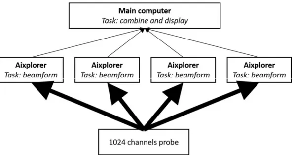
2.2. Presentation of the 3D ultrafast ultrasound scanners and probes ... 45
2.3. Development of specific tools ... 47
2.3.1. Real-time imaging ... 47
2.3.2. Visualisation tools ... 50
2.4. Conclusion ... 51
2.5. Chapter bibliography ... 53
: 3D Backscatter Tensor Imaging ... 57
3.1. Introduction ... 58
3.1.1. Motivations ... 58
3.1.2. State of the art ... 58
14
3.2. 3D Mapping of cardiac fibres orientation ... 66
3.2.1. Material and methods ... 66
3.2.2. Results ... 69
3.2.3. Discussion ... 72
3.3. Correction of aberrations due to movement ... 72
3.3.1. Material and methods ... 73
3.3.2. Results ... 76
3.3.3. Discussion ... 79
3.4. Conclusion ... 82
3.5. Chapter bibliography ... 83
: 3D passive elastography of the left ventricle ... 89
4.1. Introduction ... 90
4.1.1. Motivations: why myocardial stiffness in interesting ... 90
4.1.2. State of the art: how to measure (myocardial) stiffness ... 90
4.1.3. Objectives: non-invasive passive elastography ... 94
4.2. Material and methods ... 94
4.2.1. Simulation ... 94
4.2.2. Ultrafast Ultrasound Imaging in-vivo ... 95
4.2.3. Post processing computation ... 96
4.3. Results ... 99 4.3.1. Simulations ... 99 4.3.2. In-vivo experiments ... 99 4.4. Discussion ... 101 4.5. Conclusion ... 106 4.6. Chapter Bibliography ... 108
: 3D Ultrafast Imaging of Myocardial Contraction Activation ... 113
5.1. Introduction ... 114
5.2. State of the art, motivation, objectives ... 114
5.2.1. Electrophysiology of the heart and electrocardiogram ... 114
5.2.2. Imaging the cardiac electrophysiology ... 115
5.2.3. Imaging the cardiac contraction ... 116
15
5.3. 3D mapping ... 118
5.3.1. Material and methods ... 118
5.3.2. Results ... 120
5.3.3. Discussion ... 129
5.4. Toward clinical applications ... 129
5.4.1. Material and methods ... 130
5.4.2. Results ... 132
5.4.3. Discussion ... 138
5.5. Conclusion ... 141
5.6. Chapter Bibliography ... 143
17
Table of figures
Figure 1.1 Anatomy of the 4-chamber heart. ... 21
Figure 1.2 Origins of the main ECG segments ... 22
Figure 1.3 Examples of images obtained with cardiac MRI... 22
Figure 1.4 Coronary angiography procedure ... 23
Figure 1.5 CT imaging. ... 23
Figure 1.6 Nuclear cardiac imaging ... 24
Figure 1.7 Transthoracic echocardiography ... 25
Figure 1.8 Conventional echography technique ... 27
Figure 1.9 Illustration of the continuous Doppler principle ... 27
Figure 1.10 Visualisation of Doppler information of the carotid artery ... 29
Figure 1.11 Tissue Doppler imaging of the heart in the apical 4-chamber view... 30
Figure 1.12 Illustration of strain and strain rate imaging of the heart of a healthy volunteer. ... 31
Figure 1.13 Principle of ultrafast ultrasound imaging ... 33
Figure 1.14 Coherent compounding for ultrafast imaging ... 34
Figure 1.15 Conventional versus ultrafast ultrasound Doppler measurements ... 35
Figure 1.16 Ultrafast imaging of the pulse wave in the human abdominal aorta ... 36
Figure 1.17 3D ultrafast Doppler imaging of the carotid bifurcation of a healthy volunteer ... 36
Figure 2.1 Ultrasound scanner and probes used in this PhD. ... 46
Figure 2.2 Definition of planes or diverging waves emitted by the 2D probes ... 46
Figure 2.3 Illustration of the 2D delays law used for real-time imaging. ... 48
Figure 2.4 Real-time imaging: maximum pressure field of the beam transmitted ... 48
Figure 2.5 Comparison of 2D and 3D images quality on a phantom for real-time imaging. ... 49
Figure 2.6 Illustration of the real-time architecture ... 50
Figure 2.7 Rendering of the visualization tool developed for fibres orientation imaging ... 52
Figure 2.8. Illustrations of the results obtained with the tool developed to visualize the heart walls. ... 52
Figure 3.1 Architecture of the cardiac muscle ... 59
Figure 3.2 Schematic representation of the fibers orientation through the left ventricle wall.. ... 59
Figure 3.3 Diffusion Tensor Imaging. ... 60
Figure 3.4 Magnetic Resonance Elastography: application on a breast tumour. ... 61
Figure 3.5 Optical imaging techniques ... 62
Figure 3.6 Elastic Tensor Imaging ... 63
Figure 3.7 Derode and Fink study on fibrous composite materials ... 64
Figure 3.8 Validation of 3D-BTI against histology.. ... 65
Figure 3.9 3D-BTI: 3D representation of fibers orientation in the left ventricle of a sheep... 65
Figure 3.10 Principle of 3D-BTI: spatial coherence estimation on a 2D matrix array probe ... 67
Figure 3.11 3D-BTI associated with coherent compounding ... 68
Figure 3.12 Illustration of the analysis of the 2D coherence function using the Radon transform ... 69
Figure 3.13 Region imaged for 3D BTI ... 70
Figure 3.14: 2D coherence function of the voxel located 25mm underneath the middle of the probe ... 70
Figure 3.15 Transthoracic imaging of myocardial fibre orientation in the human heart ... 71
Figure 3.16 3D-BTI: Variations of angle across the cardiac wall thickness, in systole and diastole. ... 71
Figure 3.17 Effect of motion on coherent compounding. ... 73
18
Figure 3.19 Motion correction for 3D-BTI: workflow ... 75
Figure 3.20 Experimental setup to study the effect of motion on 3D-BTI ... 75
Figure 3.21 Schematic representation of the in-vivo acquisition to study the effect of motion on BTI ... 76
Figure 3.22 Motion estimation: evolution of estimated speed in function of ΔPW ... 78
Figure 3.23 Motion effect and correction on 2D coherence functions ... 80
Figure 3.24 Motion correction on BTI of the septum wall of a healthy volunteer at end systole.. ... 81
Figure 4.1 Schematic representation of the calculation of time-of-fight of the shear wave ... 97
Figure 4.2 Schematic representation of the calculation of distances travelled by a shear wave ... 98
Figure 4.3 Speed maps obtained from simulations ... 100
Figure 4.4 In-vivo results: propagation of natural waves during diastole and systole ... 102
Figure 4.5 In-vivo results of atrial kick on a healthy volunteer. ... 103
Figure 4.6 In-vivo results: speed maps for both volunteers for atrial kick and systole ... 104
Figure 5.1 Activation sequence of the myocardium and contribution to ECG ... 115
Figure 5.2 Sketch of Langendorff setup ... 119
Figure 5.3 Snapshots every 7ms of the velocities of the myocardium in the case of sinus rhythm. ... 122
Figure 5.4 Analysis of M-Modes of velocities and strains in a selected region of interest ... 123
Figure 5.5 Enlargement of M-Modes of velocities and strains around activation time ... 124
Figure 5.6 Activation time map of the mechanical propagation depicted figure 5.3 ... 125
Figure 5.7 Activation time maps during sinus rhythm of 3 different acquisitions of the same heart. .... 125
Figure 5.8 Snapshots every 5ms of the velocity of the myocardium 19ms after pacing time t0. ... 126
Figure 5.9 Activation map obtained when pacing ... 127
Figure 5.10 Activation maps of the same heart under the same pacing condition ... 128
Figure 5.11 Median of activation times of the myocardium, plotted against temperature ... 128
Figure 5.12 Comparison of electrical activation times measured by physiological electrodes ... 128
Figure 5.13 B-Mode of the 4-chamber view of an ultrafast ultrasound acquisition of a adult heart ... 132
Figure 5.15 ECG and M-Modes of velocities during one ultrafast ultrasound acquisition ... 134
Figure 5.16 M-Modes of velocities and accelerations during the activation of the heart ... 135
Figure 5.17 Activation times obtained on a healthy adult heart overlaid onto the B-Mode image ... 136
Figure 5.18 B-Mode image extracted from ultrafast ultrasound acquisition of a foetus ... 137
Figure 5.19 M-Modes of velocities of a foetus heart ... 139
Figure 5.20 Enlargement of M-Modes velocities around the activation time ... 140
19
:
Introduction Chapter
1. : Introduction Chapter ... 19
1.1. Introduction ... 20
1.2. Anatomy of the human heart ... 20
1.3. Clinical tools for cardiologists ... 21
1.3.1. Electrocardiogram ... 21
1.3.2. Magnetic Resonance Imaging ... 21
1.3.3. X-rays... 23
1.3.4. Nuclear medicine ... 24
1.3.5. Ultrasounds ... 24
1.3.5.1. The different cardiac views ... 25
1.3.5.2. Brightness-Mode ... 26
1.3.5.3. Continuous Wave and Pulsed Wave Doppler ... 26
1.3.5.4. Visualisation of Doppler Modes ... 28
1.3.5.5. Strain imaging ... 30
1.3.5.6. 3D imaging ... 31
1.3.6. Current limits of clinical tools ... 32
1.4. Ultrafast ultrasound imaging ... 32
1.4.1. Plane waves, diverging waves and coherent compounding ... 32
1.4.2. Elastography ... 34
1.4.3. Ultrafast Doppler ... 34
1.4.4. Imaging the propagation of natural waves ... 35
1.4.5. 3D ultrafast ultrasound imaging ... 35
1.5. Thesis objectives ... 37
20
Introduction Chapter
1.1. Introduction
Dear reader, there is about one chance over three that you will die of a cardiovascular disease. Such are the current statistics of the World Health Organisation: cardiovascular diseases (CVD) are the main cause of mortality, responsible for about one third of deaths worldwide and without surprise, early detection is key to improving their outcomes (Mendis et al., 2011). In this context, an extensive amount of researches is made to enhance the cardiac imaging techniques, and this PhD hopes to do its little bit.
In this introduction chapter, a brief description of the heart anatomy and the current imaging tools used in the clinics will be given, with a particular highlight on echocardiography and its newest developments. Among them, ultrafast ultrasound scanners and their particular applications will be introduced, as they are the foundations of this PhD thesis. The second chapter will present the 3D ultrafast ultrasound imaging material used during this PhD, and the tools developed to perform real time imaging and to visualize 3D images. The third chapter of this manuscript will present a methodology to image the cardiac muscle fibres orientation within the heart wall non-invasively. Then, the fourth chapter will be dedicated to the passive measurement of the cardiac rigidity using natural elastic waves generated during the cardiac cycle. Finally, in the fifth chapter, 3D imaging of the cardiac contraction will be performed at several thousands of frames per second for the quantification of myocardial activation delays.
1.2. Anatomy of the human heart
Through this PhD, we will often refer to the anatomy of the heart. Thus, this paragraph will give a quick introduction on cardiac structures (Figure 1.1). Mammalians heart is composed of 4 cavities (4-chamber heart) to insure blood circulation in the body. Let’s set the entry point of the heart in the right atrium (RA), in which deoxygenated blood coming from the organism is entering continuously. The blood passes into the right ventricle (RV) through the tricuspid valve. When the heart is contracting, the right ventricle ejects blood through the pulmonary valve toward the lungs. Re-oxygenated blood comes back and fill the left atrium (LA). When the atrium is contracting, the blood passes through the mitral valve and fills the left ventricle (LV). The contraction of the left ventricle ejects oxygenated blood into the organism through the aortic valve. The blood circulates within the organism before returning to the right atrium to complete the loop. For further referencing, note that the most inferior portion of the heart (i.e. the tip) is referred as the apex, and the superior part of the ventricles is referred as the basal part.
Moreover, the “right heart” (i.e. right atrium and ventricle) pushes blood to the lungs whereas the “left heart” pushes the blood to the rest of the body: the left side has a more important contraction to provide and is thus more developed that the right side. As constrains of pressure and contractility are higher, the left ventricle is the most subject to disabilities. In consequence, most of studies in the literature focus on it.
21
Figure 1.1 Anatomy of the 4-chamber heart. Image credit: Wapcaplet [CC BY-SA 3.0]
1.3. Clinical tools for cardiologists
1.3.1. Electrocardiogram
The heartbeat is triggered by an electrical pulse propagating in the heart, which path and timing are essential to the effectiveness of the heart function. The electrocardiogram (ECG) is a technique measuring the electrical activity related to the heart on the patient’s skin. In general, 3 electrodes are placed on the torso and record the well-known ECG shape (3-lead ECG). Although it may seem simple, the ECG provides many information on the heart conduction and rhythm (Figure 1.2), for a negligible cost and ease of use. Therefore, 3-lead ECG is systematically used by cardiologist as a basis for their diagnosis. For more accurate analysis, 10 electrodes may be placed on the torso: the electrical potentials can then be measured from 12 different angles (12-leads ECG), providing more spatial information. Nevertheless, despite its good temporal resolution, the spatial resolution remains limited. Moreover, the interpretation of the ECG is difficult, as pathological hearts may have a normal ECG, and abnormal ECG may be benign. Hence, for a complete diagnosis, complementary tools are used by clinicians.
1.3.2. Magnetic Resonance Imaging
Magnetic Resonance Imaging (MRI) is based on the detection of water molecules within the body. In order to do so, a strong magnetic field is exciting the hydrogen atoms of the water molecules, which in return generate radio-frequency signals. A MRI scanner is composed of a strong magnet (usually made of superconductive materials) for excitation, and coil antennas to receive radio-frequency signals, and allows the imaging of a wide range of organs of the body in 3D with a good spatial resolution.
22
Figure 1.2 Origins of the main ECG segments. The ECG shape is closely related to the path and timing of the electrical pulse activating the heart contraction. Figure from (Malmivuo and Plonsey,
1995)
Moreover, MRI is not limited by bones nor lungs as it is the case for ultrasound, and is not ionizing as PET or CT scans, making it a tool of choice for the analysis of cardiac structure (Figure 1.3) and function. However, the temporal resolution is limited: hence for cardiac applications, MRI sequences are triggered and repeated on several cardiac cycles using ECG, which implies long acquisition times and patient breath-holding. This limits the possibility of MRI scans on children, patients with breathing difficulties, or claustrophobic population. Moreover, imaging non-regular heart beats occurring in arrhythmias is challenging, although cardiac MRI is an extremely active research field and real-time MRI is being developed. Finally, the important cost of an MRI scanner restricts its availability.
Figure 1.3 Examples of images obtained with cardiac MRI. From left to right: 2-chamber long axis view, 4-chamber long axis view, short axis view. Image credits: Doregan, [CC BY-SA 4.0].
Element under copyright, diffusion not authorized Elément sous droit, diffusion non autorisée
23
1.3.3. X-rays
A few X-rays based techniques are also available to image the heart both in 2D and 3D. Angiography is a 2D X-ray technique used to image the coronary circulation (i.e. arteries and veins inside the cardiac muscle). In a nutshell, a contrast agent is injected in the coronary arteries by a catheter and a movie of X-rays images through the patient’s chest is recorded (Figure 1.4).
Figure 1.4 Coronary angiography procedure. Image credits: BruceBlaus, CC BY-SA 4.0
Computed Tomography (CT) scanners use multiple 2D X-rays images performed with different angles around the patient’s head-feet axis to reconstruct the X-ray absorption in each point of the body region scanned (Figure 1.5). Whereas in 2D the resulting image is a projection of the X-Ray absorption through the body, CT scans allow the reconstruction of 3D volumes or virtual 2D slices at desired locations. The image quality is therefore enhanced. However, the temporal resolution is relatively low, which implies the same limitations as MRI (ECG gating, long acquisition times, patient breath-holding, etc.), there is no real-time imaging (yet) and it is ionizing.
Figure 1.5 CT imaging. Scanner principle (left) and typical CT angiography 3D rendering (top right) and 2D rendering (bottom right). Images adapted from (Herman, 2009; Machida et al., 2015)
Element under copyright, diffusion not authorized Elément sous droit, diffusion non autorisée
24
1.3.4. Nuclear medicine
Nuclear medicine is sometimes referred as “radiology done inside out” because it records radiations emitting directly from the body rather than generated externally, such as X-rays. In order to do so, a radioactive tracer is injected in the organism and its radiations are captured by an external detector. Radiotracers are radioactive molecules bounded to carrier molecules, which can be chosen according to the purpose of the scan (tracking glucose, a particular protein, etc.). Thus, it allows the functional imaging of the organs rather than their anatomy: hence, nuclear imaging is often coupled with MRI or CT scans to obtain the anatomy of the organs.
As X-ray based techniques, 2D or 3D scanning are available, with similar pros and cons. Scintigraphy is a 2D method: it is simple and has a relatively low operative cost, but the contrast of the image is limited as the radioactivity signal is integrated through the width of the body. Two 3D methods based on tomographic reconstruction exist: single-photon emission computed tomography (SPECT) or positron emission tomography (PET). In SPECT, radiations are captured by a gamma camera rotating around the patients to acquire multiple 2D images at different angles. Then, a tomographic reconstruction allows for the generation of 3D volumes or virtual 2D slices. The contrast and resolution of SPECT are therefore better than scintigraphy. In PET, the radiotracer used emits positron within the body, which will annihilate with free electrons and emit two gamma photons in opposite directions. The synchronous detection of these gamma rays is performed by cameras placed on a 360°-ring around the patient. PET is known to have a better sensitivity and resolution than SPECT and is therefore considered as a gold standard in nuclear medicine, but the operating cost is more important.
Nuclear imaging techniques are mostly used to assess the perfusion of the cardiac muscle and therefore find its applications on ischemia, coronary artery diseases screening, etc.. The use of nuclear medicine is thought limited in the clinical setting by the radioactive and ionizing exposure, and the high operating cost.
Figure 1.6 Nuclear cardiac imaging. (a) Scintigraphy. (b) SPECT. (c) PET. Taken from (Zaidi, 2005)
1.3.5. Ultrasounds
Echocardiography is routinely used in the diagnosis and follow-up of cardiovascular diseases. It can provide anatomical and functional information of the heart, such as its size, shape, cardiac output, ejection fraction, diastolic function, etc. and thus, can help the detection and evaluation of cardiomyopathies. Moreover, it is relatively affordable, non-invasive, non-ionizing, and portable. In the remainder of this chapter, the principles of echocardiography and its diverse
Element under copyright, diffusion not authorized Elément sous droit, diffusion non autorisée
25
modalities will be reviewed. Then, an introduction to the cutting-edge ultrasound technologies will be presented.
1.3.5.1.
The different cardiac views
One fundamental aspect of echography is that it does not allow to image the body behind bones nor air: thus to image the heart it is necessary to avoid the ribs and the lungs, which limits the possible angles of views. Two main approaches exists: transthoracic and transesophageal echocardiography (TTE and TEE, respectively). As the names suggest, TTE images the heart through the chest of patients, whereas TEE images from the oesophagus. The main advantage of TEE is that the ultrasound beams are less attenuated and distorted before reaching the heart, hence it gives better images. However, inserting a probe through the oesophagus has important drawbacks: the patient needs to avoid eating/drinking during a few hours before the procedure, the procedure itself is time and personal consuming, and uncomfortable for the patient. For these reasons, TTE is often preferred, and TEE is used only when a better imaging quality is required.
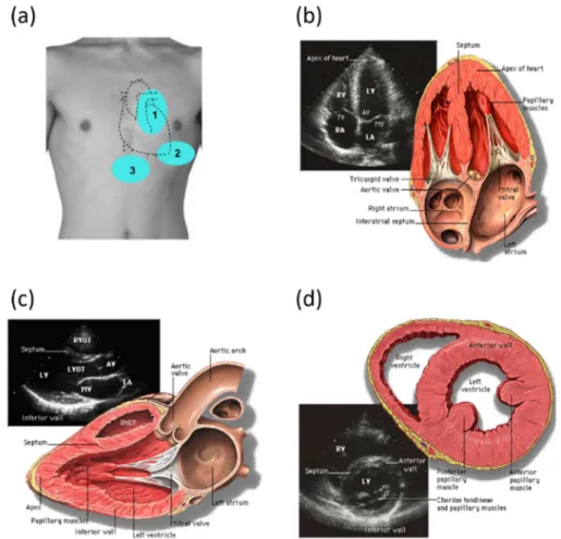
Figure 1.7 Transthoracic echocardiography. (a) Three of the acoustic windows used to image the heart. 1: parasternal, 2: apical, and 3: subcostal. (b) 4-chamber view obtained from the apical window. (c) Long-axis view and (d) short-axis view obtained from the parasternal window. To switch
between (c) and (d), the probe is rotated by 90°. RA: Right Atrium, RV: Right Ventricle, LA: Left Atrium, LV: Left ventricle, TV: tricuspid valve, AV: aortic valve, MV: mitral valve, RVOT: right ventricle outflow track, LVOT: left ventricle outflow track. Images credit: By Patrick J. Lynch and
26
In TTE, once the probe is positioned on an acoustic window (i.e. not behind bones or lungs), different views of the heart may be accessible by tilting, rotating or slightly translating the probe (Figure 1.7). For example, the apical window gives access to four different views: 2-chambers, 3-chambers, 4-chambers (Figure 1.7b) and 5-chambers views, depending on the number of structures visible. In this PhD, only transthoracic echocardiography through the apical and parasternal windows (Figure 1.7c and d) will be performed.
1.3.5.2.
Brightness-Mode
To image the human body using ultrasound, a probe consisting of several channels able to emit and receive in the MHz range is used. To form an image, the tissues are scanned line-by-line by a focused ultrasonic pulse (typically a few periods of the central frequency of the probe). Along the beam, echoes are backscattered by local variations of acoustic impedance, and received by all the elements of the probe. By applying simple delay laws, the echoes are focalized in reception and the echogenicity of the medium along the scanning line can be retrieved. This process is then repeated about a hundred times to scan laterally the medium to obtain a complete image (Figure 1.8). The Brightness-Mode imaging (B-Mode) consists of displaying the intensity of the received echoes from each pixels via a black-to-white scale, the brightest points representing the most echogenic tissues (see examples of Figure 1.7).
A wide variety of probes can be found depending on the clinical applications. In particular, so-called phased-array probes are dedicated to cardiac imaging and are characterized by:
a low central frequency to ensure a good penetration depth (in the range 1-3MHz to reach ~15cm),
small channels width relative to the wavelength of the ultrasonic pulse (typically 𝜆 2) to allow the emission of diverging waves and therefore widen the angle of view of the probe1,
a limited number of channels (e.g. 64) to be able to place the probe in-between ribs.
1.3.5.3.
Continuous Wave and Pulsed Wave Doppler
A number of methods allow for the estimation of movements, which we will briefly review bellow. Continuous wave Doppler (CW)
The first method developed was based on the Doppler effect, the same that distorts the sound of rapidly passing cars in the street. The probe is made of two transducers slightly angulated, one of them emitting continuously a focalized ultrasound wave, whereas the other is recording continuously the echoes.
1 Considering a 1.5MHz probe and a speed of sound in biological tissues of 1540m/s, the typical lateral
27
Figure 1.8 Conventional echography technique. Ultrasound image formation using (a) a linear probe and (b) a cardiac probe. Image taken from (Correia, 2016)
If scatterers are moving axially within the zone covered by the two focalized transducers, the frequency of the ultrasound beam received if shifted by a frequency 𝑓 compared to the emitted frequency 𝑓 . 𝑓 is the Doppler frequency and is given by:
𝑓 =2𝑣 𝑐𝑜𝑠𝜃
𝑐 𝑓 (1)
where 𝑣 is the axial velocity of scatterers, 𝜃/2 the angulation of the transducers compared to the z-axis (see Figure 1.9) and 𝑐 the speed of sound in biological tissues. Fortuitously, the Doppler frequency 𝑓 obtained by measuring blood flow circulation is the audible frequency range (~kHz). Thus, at the beginning of echocardiography, very simple and effective ultrasound scanners could calculate analogously the Doppler frequency and play the resulting signal through speakers. Up-to-date, this typical sound is still used by clinicians (along with other tools, fortunately). CW can measure high blood velocities (up to 1.5m/s) and is therefore still used nowadays to analyse the velocity of blood ejected from the heart through the aorta. In modern systems, CW can be performed on imaging probes by using subapertures: half of the channels of the probe are used as transmitters and the other half as receivers.
Figure 1.9 Illustration of the continuous Doppler principle. The blue zone represents the field of view in which the movement can be estimated. Note that the angle θ has been exaggerated for illustration
purposes. In practice, the recovering ultrasonic beam is narrow and has a large depth.
Element under copyright, diffusion not authorized Elément sous droit, diffusion non autorisée
28 Pulsed wave Doppler
Pulsed Wave Doppler (so-called pulsed Doppler) relies on different physics: as its name suggests, it is based on pulse-echo measurements. Focalized ultrasonic pulses are send to the medium and the echo are correlated to estimate the motion of scatterers along the beam (Baker, 1975). This method can be used with a unique transducer to provide a 1D image of movement along the beam (1D pulsed Doppler), or a linear array and thus a 2D image can be reconstructed in a similar manner as a 2D B-Mode images are made. Fortuitously, the frequency of the oscillations of the beamformed signals is related to the medium’s velocity by the same equation (1), although the mechanisms implied are different. Finally, in pulsed Doppler, a fundamental parameter is the pulse repetition frequency (PRF), as it defines the limit of velocity estimable without aliasing, according to the sampling theory: 𝑃𝑅𝐹 ≥ 2𝑓 . To work around this limitation, pulsed Doppler modes are firing several times the same scan lines of the image before sweeping to the next ones, allowing a high PRF but with a limited number of samples for each scan line. The number of transmits for each scan lines depends on the mode used, whether precise estimation in a small area or qualitative imaging in a larger area is desired. The different modes will be discussed in the following paragraphs.
Moreover, the pulsed Doppler technique described here may be applied to blood flows (Figure 1.10) or tissues motion (Figure 1.11). The latter is notably useful in echocardiography, where the estimation of motion of cardiac wall and mitral valve annulus has been investigated since the development of Doppler techniques (Isaaz et al., 1989).
To summarize, CW has the advantages of being able to measure high velocities but lacks spatial information, whereas pulsed Doppler is limited by the PRF but allows localization in space.
1.3.5.4.
Visualisation of Doppler Modes
Until now, we described how to estimate motion without discussing how to visualise it. Data visualisation is crucial for the effectiveness of a technique, and depends on the information to be extracted from the data, and from the nature of the data itself.
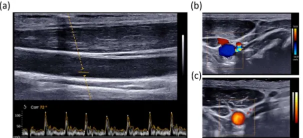
Quantitative analysis: Spectral representation
The first method to visualize motion was used on CW and pulsed Doppler and consisted of displaying a spectrogram of the Doppler signal received (Figure 1.10a). In the case of pulsed Doppler, measurements of motion are made in a few pixels wide region of interest (ROI) manually selected on the B-Mode image by the operator, and the spectrogram is calculated in these pixels. The small size of the ROI allows to repeat a high number of focalized transmissions along its scan line, improving the sampling of the Doppler signal and thus the quality of the spectrogram, but is preventing to form an image of motion. The spectrogram is the method of choice to measure blood flow velocities, as well as cardiac synchronisation (e.g. delay between peak velocities across the different valves). Note that this technique is often referred as “pulsed-Doppler” itself; to avoid this ambiguity, we will refer to it as “spectral” Doppler in this document.
29
Visual analysis: Colour Doppler and Power Doppler
Colour Doppler and Power Doppler aim to image motion in 2D (or 3D). Therefore, pulsed Doppler measurements are repeated along several scan lines which implies a limitation: the bigger the region of interest selected, the less focalised transmission can be repeated for each scan lines, to maintain a sufficient PRF. Hence, the measurements cannot be as precise as in the case of spectral Doppler. Moreover, as the PRF is lower, so is the maximum velocity measurable. Each pixel in the specified region of interest has a specific colour-assigned value overlaid onto B-Mode images depending on Doppler data.
In the case of colour Doppler, the central frequency of the Doppler signal of each pixel is calculated and color-coded on the image. By convention, the colour axis goes from blue to red to represent motion away and toward the probe, respectively (Figure 1.10b). The estimation of velocity and axial direction is of great interest to understand the blood circulation organisation (for example in the brain), the displacement of tissues (free walls of the heart) or turbulences associated to high speed flows (carotid arteries, cardiac valves …).
Power Doppler is another methodology to visualize motion which associates at each pixel the energy of its Doppler signal. By doing so, both directional and quantitative information about flow velocity are lost, however the sensitivity of the resulting image is enhanced. Therefore this mode is appreciated to visualize vessels architecture. Power Doppler is usually encoded in a red to white colour axis (Figure 1.10c).
Thus, depending on the information investigated by the operator, CW and spectral representation, or pulsed Doppler and one of its visualisation method may be used: to measure precisely velocities, CW or pulsed Doppler spectral representation would be preferred, colour Doppler would be chosen to investigate motion directions and flow turbulences, and finally power Doppler to image the architecture of the vessels. The main pros and cons of each modality are summarized-up in Table 1-1.
Figure 1.10 Visualisation of Doppler information of the carotid artery. (a) Spectrogram of the carotid blood flow through a small ROI. (b) Colour Doppler and (c) Power Doppler of the radial view of the
30
Figure 1.11 Tissue Doppler imaging of the heart in the apical 4-chamber view. (a) Colour Coded images of tissue Doppler and visualisation of tissue velocity versus time of selected points of the wall.
(b) Spectral Doppler of one point of the image, near the aortic valve. Image adapted from (from Yu et al., 2007).
Spectral Doppler Colour Doppler Power Doppler
Examines flow at one site Good temporal resolution Allows calculations of velocity
Overall view of flow in a region Poor temporal resolution Approx. velocity information Direction information Turbulent flows
Overall view of flow in a region Poor temporal resolution No quantitative velocity No directional information Sensitive to slow flows Table 1-1 Summary of main proprieties of pulsed Doppler modes.
1.3.5.5.
Strain imaging
Based on the tissue motion estimates, one can calculate its deformation (strain), which is of great interest in the case of the heart, as both important motion and deformation occurs during the cardiac cycle and are fundamental for its function. The underlying principle is fairly simple: the aim is to compare the motion of close points in the tissues: if two points get closer with time, the tissues slims, if they get further, the tissue thickens. Several techniques can be used to estimate strain (or strain rate) using ultrasound. The first one is directly derived from pulsed Doppler as it is based on the analysis of the phase-shift of the received echoes from the regions of interest (Kanai et al., 1997). It has the advantages of being simply implementable and has a great axial sensitivity, but is restrained to axial estimation. The second method is inspired from particle image velocimetry, which was developed in optics: it consists of tracking local scatterers in the beamformed image to compute their movement and thus the local strain (Meunier et al., 1989). As the local aspect and “granularity” of ultrasound images is called speckle, this technique has been named speckle tracking. The advantages of speckle tracking is that it can estimate motion in all dimensions of the image, and so it can compute longitudinal and shear strain. For a 2D image, 4 strain components can be derived, and up to 9 components for 3D volumes, allowing for the complete description of the tissues deformation. Up-to-date, 2D strain has been shown to be a good tool to assess cardiomyopathies (Nesbitt et al., 2009) and is more and more used in the clinics. An illustration of strain imaging of the heart is presented Figure 1.12.
Element under copyright, diffusion not authorized Elément sous droit, diffusion non autorisée
31
Figure 1.12 Illustration of strain and strain rate imaging of the heart of a healthy volunteer. Left: strain rate image overlaid onto B-Mode in the apical 4-chamber view. Time profiles of strain rate
(middle) and strain (right) at 3 different positions along the interventricular septum during a complete cardiac cycle. AVC: aortic valve closure. MVO: Mitral valve Opening. (D’hooge, 2000)
1.3.5.6.
3D imaging
One of the limits of ultrasound imaging compared to its best competitors (MRI, CT, etc.) is that most of the scanners currently in use are limited to 2D imaging. However, 3D imaging is possible and desirable. The major reason for the need of 3D ultrasound is to overcome the limits of viewing in 2D the 3D anatomy. Indeed, with 2D imaging the operator needs to integrate multiple 2D images in his/her mind to reconstruct the 3D anatomy, which is inefficient and may lead to variability and incorrect diagnoses, especially for echocardiography where a limited number of views are available.
The main advantages of 3D include:
Volume rendering and segmentation
Arbitrary 2D slices of the volume may be visualized (not only in the plane defined by the probe, which is the case in 2D). Moreover, 2D slices can be recomputed and visualized a posteriori.
Visualization of complex geometry (e.g. tumours vascularisation)
Precise measurements of metrics (length, radius, volumes, …) with reduced inter-operator dependence
Element under copyright, diffusion not authorized Elément sous droit, diffusion non autorisée
32
Up-to-date, two main techniques exist to perform 3D ultrasound imaging: moving a 2D transducer to obtain multiple 2D images, or using a dedicated 3D matrix probe. The former case can again be divided into subcategories, depending on the way the 2D images through the volume are obtained: one possibility is to scan freely move the probe on the patient’s skin and recombine the images using correlation algorithms (Downey and Fenster, 1995). In this case, some systems may integrate a tracking device to register the movement of the probe (Mercier et al., 2005). The other subcategory consists of building a “virtual” 3D probe consisting of a linear array that can be either translated, rotated or tilted by a motor to scan the volume. Finally, in the second main technique a dedicated 3D probe composed of a 2D matrix of ultrasonic transducers is used, allowing to directly image the volume below the probe. In a similar manner than with phased-array probes, diverging waves can be emitted to extend the field of view to a pyramidal shape. This solution implies a high number of transducers: to be used with standard ultrasound scanners, electronics are integrated within the probe to pre-process the signals and reduced the number of channels to be sampled. Once 3D volumes acquired, the 2D techniques detailed above can be directly applied to obtain volumetric Doppler, strain imaging, etc..
Studies have shown the potential of 3D ultrasound imaging for cardiac applications on foetuses and adults hearts, but it is however still limited by the low framerate (Lang et al., 2012; Yagel et al., 2007).
1.3.6. Current limits of clinical tools
Although the large number of tools available to clinicians to examine the heart, each of them has drawbacks and limitations. An ideal imaging tool would be: cheap, non-ionizing nor invasive, 3D and with a good temporal resolution.
1.4. Ultrafast ultrasound imaging
1.4.1. Plane waves, diverging waves and coherent
compounding
In the following paragraphs, we will present ultrafast ultrasound imaging, to be opposed to conventional ultrasound. In the latter, we saw that an image is formed line by line, so the maximum framerate is limited by the necessary time to form one line (i.e., the depth of the image) multiplied by number of desired lines. Ultrafast imaging relies on the insonification of the whole region to be scanned in one ultrasound transmission. Therefore, the time to form an image is only limited by the time-of-flight necessary for the wave to travel back and forth the depth of the image. If the desired image has N=100 lines, ultrafast imaging allows to multiply the framerate by a factor N=100, allowing to reach up to 10.000 frames/seconds. For linear array probes, a plane wave is transmitted to scan the medium directly below the probe, whereas
33
diverging waves can be sent by phased-array probes to image a wider sector2 (Figure 1.13). To
form the image, the echoes are processed by a conventional delay-and-sum beamformer. The drawback of ultrafast imaging is that as the transmitted beam is not focalized, the contrast and the resolution of the resulting image is lower than what is obtained with conventional ultrasound imaging.
Figure 1.13 Principle of ultrafast ultrasound imaging. The whole medium is insonified by only one ultrasound pulse. The wave sent by the transducer can be plane for linear probes (a) or diverging for
phased-array probes (b). Figure from (Correia, 2016).
To overcome these limits, Montaldo et al., suggested the transmission of multiple tilted plane waves. Their coherent compounding in post-processing is equivalent to synthetic focusing in emission, as illustrated on Figure 1.14 (under the assumption that there is no significant movement in between their transmissions, as we will discussed later in chapter 3). By doing so, both contrast and resolution can be enhanced and compared to conventional ultrasound imaging, while the framerate is still significantly higher (Montaldo et al., 2009). As always, a trade-off has to be made: the higher the number of plane waves used, the better the synthetic focusing and hence the resulting image, but the lower the framerate. Thus, the choice of the number of plane waves is made according to the experimental requirements: typically, about 40 plane waves are sufficient to retrieve a quality equivalent to conventional ultrasound.
That being said, one could legitimately wonder the point of generating real time images at thousands of frames per seconds. Thus in the following paragraphs, we will introduce some applications made possible by ultrafast ultrasound imaging.
2 Note that for the sake of simplicity, we will refer to plane waves to further describe this technology in
this manuscript, but all the developments can be applied on diverging waves too.
Element under copyright, diffusion not authorized Elément sous droit, diffusion non autorisée
34
Figure 1.14 Coherent compounding for ultrafast imaging. (a) A series of plane (or diverging) waves are emitted, and echoes are recorded for each transmission. In post-processing, plane waves can be synthetically focused in any pixel of the image (b), (c), (d). Image from (Montaldo et al., 2009).
1.4.2. Elastography
Elastography is a technique consisting of measuring the stiffness of tissues. One of the primary application of ultrafast ultrasound was the imaging of the propagation of shear waves within the body (Shear Wave Elastography, SWE). Indeed, the shear wave speed is a good way to assess the rigidity of the tissues in which they travel, which is a relevant marker to detect pathologies. In the human body, shear waves travel at speeds in the range 1 to 10m/s: thus they propagate through the field of view of ultrasound within a few milliseconds. Hence, ultrafast framerate (>1000frames/second) are required to correctly image their motion and estimate their speed in a 2D region of interest. The proof of concept of imaging shear waves propagation (Sandrin et al., 1999), local shear modulus calculation (Sandrin et al., 2002), and medical application on breast cancer detection (Bercoff et al., 2003) were developed in our group in parallel to the emergence of 2D ultrafast ultrasound imaging. For a more detailed introduction to elastography, please refer to the chapter 4 of this thesis.
1.4.3. Ultrafast Doppler
A few years after the developments of elastography, ultrafast ultrasound was also applied to Doppler imaging (Bercoff et al., 2011). Indeed, we saw that pulsed Doppler modes were limited by the size of the region of interest in which Doppler measurements are made. Ultrafast imaging allows to overcome this limit as it provides a continuous sampling at a high PRF for each pixel of the image, which makes possible the computing of all Doppler modalities in each point: spectral, colour and power Doppler (Figure 1.15). Therefore, although it may seem surprising at the first time, the high framerate brought by ultrafast ultrasound improves the imaging of slow motions as well. Applied to brain imaging, it led to high sensitivity mapping of cerebral blood volume and functional ultrasound (Macé et al., 2011; Mace et al., 2013; Demené et al., 2014).
Element under copyright, diffusion not authorized Elément sous droit, diffusion non autorisée