Science Arts & Métiers (SAM)
is an open access repository that collects the work of Arts et Métiers Institute of Technology researchers and makes it freely available over the web where possible.
This is an author-deposited version published in: https://sam.ensam.eu Handle ID: .http://hdl.handle.net/10985/11351
To cite this version :
Jean-Philippe PERNOT, Franca GIANNINI, Cédric PETTON - Categorization of CAD models based on thin part identification - In: Tools and Methods for Competitive Engineering, Allemagne, 2012 - Proceeding of TMCE 2012 - 2012
Any correspondence concerning this service should be sent to the repository Administrator : [email protected]
CATEGORIZATION OF CAD MODELS BASED ON THIN PART IDENTIFICATION
Jean-Philippe Pernot1, Franca Giannini2, Cédric Petton1,2
1Arts et Métiers ParisTech
Laboratory LSIS - UMR CNRS 6168 FRANCE
2Istituto di Matematica Applicata e Tecnologie
Informa-tiche, Consiglio Nazionale delle Ricerche ITALY
ABSTRACT
Nowadays, industrial CAD models databases are becoming larger and larger, thus inaugurating new challenges for their management during the product design process. Unfortunately, neither the PDM nor PLM systems are good at indexing and sorting CAD models according to their content, and it is sometime more efficient to redesign a part than to try to find it in a database. Categorizing parts is a first step to solve this problem. This may allow both the re-use of the parts and the retrieval of the methods and pro-cesses adopted on them, thus avoiding wasting time restarting from scratch. In this paper, we focus on the characterization and classification of industrial parts with respect to the meshing issue, and notably the meshing of thin parts difficulty handled automati-cally and which often requires adaptation steps. The concepts of thin object and thin part are introduced together with the mechanisms and criteria used to identify such shape characteristics on CAD models. The final categorization results of a set of tests ex-ploiting a normalized distance distribution associat-ed to specific ratios computassociat-ed from the bounding box surrounding the object to be classified. The proposed approach has been implemented and validated.
KEYWORDS
CAD models categorization, shape characteristics, thin features and objects, distance and shape distribu-tions.
1. INTRODUCTION
Today, the methods and processes used all along the product design process end up with the generation and manipulation of a huge amount of digital data used to simulate the entire product lifecycle. In this framework, the geometric models are the intermedi-ate representations shared by most of the actors. Therefore, large databases of CAD models are be-coming available, thus inaugurating new challenges
for their management. For example, the complete digital mock-up of the airplane Airbus A400M is made up several hundreds of thousands of parts rep-resenting several terabytes of data.
Consequently, there exists an increasing need for indexing and sorting those elements to be able to retrieve them efficiently later on. Unfortunately, nei-ther the actual PDM nor PLM systems are good at indexing and sorting CAD models according to their content, i.e. according to the shape. Indeed, it is not possible to find a part only with the filename, fre-quently unknown, or some annotations, possibly missing or limited for the specific purposes. Thus, the best method to retrieve a part is to exploit the shape characteristics. But, even the shape might be misleading or not enough. Depending on the purpos-es, we might be interested in parts, possibly very different in the overall shape, but similar according to some characteristics or behaviours. It is therefore necessary to provide tools enabling context-based shape categorization. Such a categorization can then provide a good mean for the re-use of past experi-ences and knowledge related to specific products or activities. In this paper, we are considering a catego-rization of the CAD models according to the meshing issue.
Product structural analyses are classically carried out following three steps: the CAD model definition, its meshing and the FE simulation including the bounda-ry conditions specification. Before the meshing, the CAD model may also be idealized and simplified to remove unimportant features, i.e. features that will not affect significantly the simulation results. In this context, having tools to categorize parts according to the required types of adaptation could help the engi-neers in better and faster preparing their models to the meshing step. Actually, when meshing complex parts, two main steps have to be distinguished: ‐ the adaptation step aims at preparing the CAD
models to the meshing and simulation while per-forming dedicated transformations. One example
concerns the de-featuring of the CAD models to reduce the computation time by removing unim-portant features which do not affect significantly the simulation results;
‐ the adjustment/repairing step aims at improv-ing the quality of the produced meshes while re-moving and/or repairing some badly meshed el-ements. This is a time-consuming step often per-formed manually using operations such as re-moval, swap, local refinement and so on.
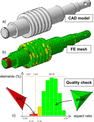
Therefore, having tools to distinguish parts that have to be adapted and/or repaired manually from those that can be meshed automatically would speed up the simulation model preparation steps. Here, the pro-posed categorization method separates thin parts, or parts with thin features, from parts with a rather con-stant and consistent thickness with respect to the parts’ size. This criterion has been defined to antici-pate the problems occurring when creating tetrahe-dral meshes from CAD models with different thick-nesses and particularly when a thin feature is linked to a large volume. Effectively, such configurations can generate a bad quality meshing often responsible for inaccuracies during the simulation. The meshing of the endless screw of figure 1.a illustrates this prob-lem. Indeed, there exist thin parts at the end of the screw thread as well as around the chamfer. Depend-ing on the targeted size of the elements, tetrahedra with a bad aspect ratio [6] may have been generated (fig. 1.c). Since these processes are not fully auto-mated, designers still have to act on many control parameters. For instance, they have to determine the best size of the elements, because the meshing tools often suggest a default size which does not take into account thin features.
However, the work exposed in this paper aims nei-ther at preparing the CAD models nor at repairing the FE meshes. Again, the objective is to categorize CAD models to better anticipate the adaptation and repairing steps. In this way, designers spend more time to treat critical models on which thin parts have been highlighted. Using this approach, they can also look for already applied solutions by retrieving simi-lar parts in huge databases.
This paper is organized as follows. Section 2 intro-duces the proposed categorization approach as well as the state-or-the-art of the existing methods. The considered object categories are presented in section 3 and the shape descriptors used to characterize those objects are detailed in section 4. The way those shape descriptors are combined to define higher-level
ob-ject categories is detailed in section 5. Finally, sec-tion 6 details the achievements and results we obtain using our prototype software.
a) CAD model b) FE mesh aspect ratio Quality check elements (%) bad good c)
Figure 1 Meshing of thin parts (a) producing bad quality
tetrahedral meshes (b, c).
2. RELATED WORKS
The 3D shape retrieval has recently gained big atten-tion due to the fact that large databases of 3D data are becoming available in various fields. Unfortu-nately, current methods for 3D shape retrieval are mostly focusing on the similarity of shapes from the form and structural point of views. Indeed, lots of shape matching methods exist [1-3, 8-9] and can be classified in three main categories: feature-based methods, graph-based methods and geometry-based methods (see figure 2). These methods have been implemented and tested. The results are more or less efficient but only when trying to retrieve a shape similar to the one of the query. Instead, to support a more application-oriented retrieval, we define a method to categorize parts with criteria not based on simple shape similarity but on specific shape distri-bution characteristics impacting on the meshing. Therefore our method can have impact in a concrete application in virtual mechanical engineering.
Figure 2 Taxonomy of shape matching methods [1].
In our approach, two steps can be distinguished. The first step consists in extracting shape distribution characteristics from a set of vertices obtained by discretizing the surfaces of the B-Rep CAD model to be categorized. The second analyses the descriptor values to determine the appropriate category for the considered object. Thus, our approach can be seen as belonging to the global feature distribution category (fig. 2).
Actually, the global feature distribution method con-sists in comparing the distribution of global features instead of the global features directly. Among the existing methods, the one of Osada et al. [4] intro-duces the so-called “D2 Shape Distribution” to repre-sent, in a normalized histogram, the probability of occurrence of Euclidean distances between pairs of points chosen randomly on the skin of the object. This probabilistic approach is easy to implement, the computation speed is fast, and it is invariant to geo-metric transformations. As explained in section 4.1, this descriptor has been adapted to our needs.
However, such a distribution only characterizes the overall shape of the object and not the details. This is why the method is not sufficiently efficient to catego-rize parts with particular features. Therefore, we have been using another descriptor: the Oriented Bounding Box (OBB). The OBB (in opposition to axis-aligned minimum bounding box) is a descriptor introduced by Chang et al. [5] in an article suggesting some methods to compute it, like the most popular class of heuristic methods: the Principal Components Analy-sis (PCA). Because of its easy implementation and its good results for the considered parts, the most basic of the PCA-based methods has been adopted. Indeed,
when computing the bounding box, our aim is to get the volumetric ratio between the model and its mini-mal OBB. This indicates whether the object incorpo-rate empty parts or not. We also use the dimensions of the bounding box to characterize some kind of features, as widely described in the following sec-tions.
Finally, when considering the 3D models processing and retrieval methods [1-3], one can notice that they are working with a wide variety of 3D geometric representations (e.g. points cloud, polygons soup, structured meshes). However, most of the models found on the Internet are polyhedral models defined in a file format supporting the visual appearance. Today, the most common format used for this pur-pose is the Virtual Reality Modeling Language (VRML) format. Since this format has been designed for visualization, it only contains geometric and ap-pearance attributes. In our approach, to be as much as possible independent of the adopted CAD software, we are working on polygons soups exported from in a stereolithography (STL) file format. STL models are not watertight meshes, i.e. they do not enclose a volume. So the algorithm developed is able to com-pute descriptors on a soup of triangles (polygons), thus it can easily deal with most of 3D models avail-able over the web.
3. CONSIDERED OBJECT CATEGORIES
To define which categories of objects have to be considered, the different treatments and possible problems that can occur when meshing a CAD model have been analysed. In particular, three main catego-ries of objects have been identified at first (fig. 3): ‐ the globally thin objects (fig. 3.a);
‐ the objects containing so-called thin parts much thinner than the rest of the object (fig. 3.b); ‐ the normal objects, i.e. those not belonging to
the two above mentioned categories (fig. 3.c). As discussed in the introduction, the first and second categories gather together CAD models that can be subjected to some idealisation processes and whose meshing may require manual adjustment steps. The second category also includes objects deserving par-ticular attention for the choice of the mesh size. To-day, the last category gathers together all the CAD models that do belong neither to the globally nor locally thin objects categories, despite the fact that their meshing can still be problematic. Therefore, in
the future, new categories have to be imagined to further categorize the actual “normal objects”.
a)
Thin objects Objects with thin parts
b) c)
Normal objects
Figure 3 Examples of objects of the identified three
cate-gories: globally thin objects (a), objects with thin parts (b) and normal objects (c).
According to the characterizing features of the above classes, various existing shape descriptors have been analyzed and the most meaningful for their identifi-cation have been considered. They include the vol-ume, the dimensions, and the thicknesses of the parts. The next section introduces the developed descriptors as well as the method used for their computation.
4. ADOPTED SHAPE DESCRIPTORS
4.1. Volume of the model
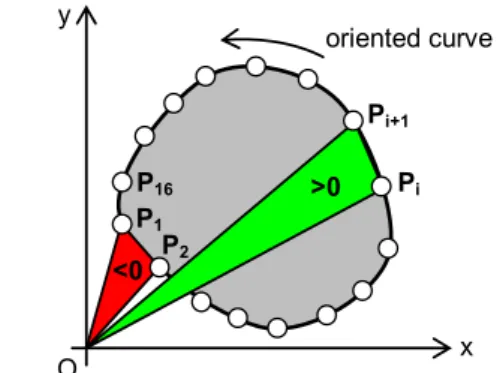
The method used to compute the internal area of a closed planar curve can be extended to compute the volume of a 3D closed B-Rep model. In 2D, the in-ternal area of a closed curve can be computed while dividing the oriented bounding curve in several seg-ments [PiPi+1] (fig. 4). For each oriented segment, an
oriented triangle PiPi+1O is built using the origin O of
the reference frame as third vertex. The signed area of those oriented triangles can be computed using a simple vector product (^) as follows:
(1) The internal area of the curve is then computed by summing up the signed areas:
(2) In 3D, the principle is similar. Instead of computing the area of oriented triangles, we sum up signed vol-umes of oriented tetrahedra. Each tetrahedron has a
base defined with an oriented triangle and the origin of the reference frame as forth vertex.
x y O Pi Pi+1 oriented curve P1 P2 P16 >0 <0
Figure 4 Computation of the area inside a closed curve.
4.2. Bounding Box
The first descriptor chosen from literature is the min-imal oriented bounding box. It consists, given a finite set of N points, in finding the cuboid, i.e. rectangular parallelepiped, of minimal volume enclosing the set of vertices defined on the object surface.
To get this oriented bounding box, we decided to use a famous and basic but nevertheless efficient method which is the Principal Components Analysis (PCA). The PCA is mathematically defined as orthogonal linear transformation that transforms the data to a new coordinate system such that the greatest variance by any projection of the data comes to lie on the first coordinate (called the first principal component), the second greatest variance on the second coordinate, and so on. The principle of the PCA consists in com-puting the covariance matrix of the set of vertices. Then the three axes (vectors) of inertia are obtained by computing the eigenvectors of the covariance matrix. The last element is the center of gravity, whose coordinates (XG, YG, ZG) are the mean of the
coordinates (X, Y, Z) of the set of points.
Given the three axis of inertia and the center of gravi-ty of the model, the three dimensions of the bounding box can be computed. Indeed, the method consists in projecting all the points on the three axes of inertia, and then measuring the longest distance between projected points of the axis. It is done by creating, for each point of the model, a vector from the center of gravity to the point, and then by computing and stor-ing in a list the dot product between these vectors and the three eigenvectors (normed vectors). From this list of oriented distances, the difference between the maximum and the minimum represents one distance of the bounding box. Then, with this information, it is possible to build the bounding box.
This bounding box is used in combination with the part volume as a descriptor giving information on the filling of the model in its bounding box. Also, the proportions among the dimensions of the bounding box reveal if the bounding box of the part is more like a plate (thin) or like a cuboid.
The combination of these descriptors is described in further details in a following section.
4.2.1. Enclosing surface area
The area of the model is used in the distance distribu-tion, and is computed by summing the area of each triangle face of the model.
4.2.2. Distance distribution
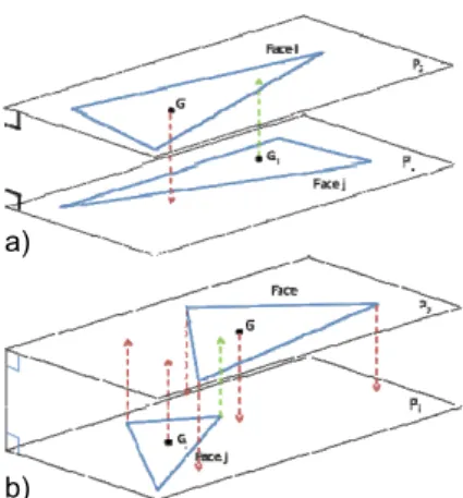
One of the main descriptors used in our work is the distance distribution, inspired from the work of Osa-da et al. [4] on the D2 shape distribution descriptor. With this distribution, it is possible to characterize the overall shape of the object and to retrieve a simi-lar shape. That means that the designer has to create its “categories” of models before being able to rec-ognize a new one. In this work, the aim is to recog-nize features on subparts of the shape or on the entire shape. So, we have adapted the idea of computing distances inside the model, but with some conditions allowing us a characterization of the object features. The aim of this descriptor is to compute the thickness inside the part. The main difference with the D2 shape descriptor is the fact that we compute distance between faces and not vertices and with some addi-tional conditions. For each face of the model, the algorithm checks the parallelism between faces. In-deed, the distance between two faces needs to be defined when the two faces are not parallel. Thus, the developed algorithm acts differently according to the two cases: when faces are almost parallel, or when the angle between the two normals is less than 60°. When faces are almost parallel, we first check if the faces are facing each other, and this to avoid irrele-vant distance computations. We use a method which consists in projecting the three points and the center of gravity of one face into the other one. If the pro-jection of center of gravity of a face lies inside the other face, like in figure 5.a, we consider that the distance computation is useful for the thickness dis-tribution. Moreover, by using the opposite of the normal vector to the face for projecting the center of gravity, the algorithm allows the differentiation be-tween parallel faces enclosing the object material or
the void. Indeed, we do not care of distance between parallel faces not enclosing the object material.
a)
b)
Figure 5 Parallel faces identification with projection of
the gravity center of the triangle (a), and projection of the face vertices (b).
When no gravity center is projected in the other face, the algorithm verifies if at least the projection of one of the three vertices of the face is inside the other face (fig. 5.b). Actually, there is a case which is not taken into account, when the two faces are facing but all the projections (center of gravity and other points) are not lying in the other face. This is not a critical issue because we assume that if a triangle face fi is in
this case with a face fj, fi (or fj ) is almost parallel to a
face adjacent to fj (resp. fi).
So the algorithm reviews each faces, one by one, and carries out the above tests before computing the dis-tance. The distance is then evaluated by computing the dot product of the vector between the two centers of gravity and the outward-oriented normal vector of the tested triangle.
In case of non-parallel faces, i.e. when the angle be-tween the two faces is bebe-tween almost 10° to 60°, the considered distance is the smallest one between the three points of each faces. In this way, it is possible to recognize features as those in figure 3 where the thickness requires a check before meshing, then to categorize these parts and it is the purpose of next section. The values for distinguishing parallel from non-parallel faces have been heuristically chosen to get rid of approximation problems.
With these tests and this function, lots of irrelevant results are avoided. The distance distribution is then made tessellation-invariant by using the surface of the triangle associated to the distance: when the above described conditions are satisfied and a dis-tance can be computed between a face fi and a face fj,
the faces fi and fj. At the end, all the areas associated
to the same distance are summed and normalized by the value of the total object surface area. In this way it is possible to know how much surface (% of the total surface) is linked to the same thickness.
Figure 6 shows two examples of very simple parts with the associated thickness distribution function and the filling of their respective bounding boxes. The first model (fig. 6.a) is a cuboid with a rib, the percentage of the volumetric filling of its bounding box is equal to 0.74. The thickness distribution re-veals only three distances inside the model. The x-axis indicates the value of the thickness divided by the diagonal of the bounding box, while the y-axis represents the area percentage. We decided to use the bounding box diagonal in order to make comparable objects of very different dimensions. The second model shows that also for very curved parts we can get meaningful values (fig. 6.b).
Vmodel Vbb = 0.21 Thickness (%) Vmodel Vbb = 0.74 Thickness (%) Area (%) a) b) Area (%)
Figure 6 Examples of shape distribution functions.
5. PART CATEGORIZATION
In this section we illustrate how the descriptors intro-duced in section 4 have been used to define the membership function to categorize objects according to the classification described in section 3. This
membership function uses some thresholds which have been defined empirically (see section 5.3). Let’s define the different terms used in the following subsections:
‐ VM : the volume of the model;
‐ VBB : the volume of the bounding box;
‐ DBB1,DBB2,DBB3 : the dimensions of the
bound-ing box so that DBB1 ≥ DBB2 ≥ DBB3;
‐ diagBB : the diagonal of the bounding box;
‐ F[x ; y] = z : function of the distribution so that there is z% of the total area of the model associ-ated to distances between x% and y% of the di-agonal of the bounding box. For example, writ-ing “F[0 ; 0.25] = 0.88” means that “88% of the total surface is associated to a thickness between 0 and 25% of the diagonal of the bounding box”.
5.1. Thin parts
The thin part class includes different types of objects, such as those similar to thin plates, or having an arbi-trary shape with almost constant thickness distribu-tion, or presenting a large emptiness of the bounding box (fig. 7). Different criteria are used to distinguish the typology of thin objects, as described in the fol-lowing. Clearly, some thin objects can satisfy more than one criterion simultaneously.
a) b) c)
Figure 7 Examples of thin objects.
The first criterion (crit.1 in table 1) identifies plates, based on the fact that plate-like objects have one of the three dimensions of the bounding box quite small with respect to the two others, with a part filling at least the half of its bounding box. This criterion al-lows the identification of thin parts (fig. 7.a).
The second criterion (crit.2 in table 1) aims at con-sidering thin objects having two of the bounding box dimensions quite similar while the third is rather small and including large part of material inside the part bounding box. Therefore, the conditions to be satisfied are: (VM / VBB < 0.8) & (DBB1/DBB2 < 1.75)
7.a and7.c are also kept by this criterion in the thin part class.
The third criterion (crit.3 in table 1) considers objects having a general overall shape with no predominant dimension of the bounding box and so that VM / VBB
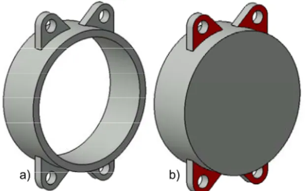
< 0.2. This kind of objects is characterized by the fact that the volume occupied by the part in the enclosing bounding box is just a small part (volumetric differ-ence under 20%). The aim is to catch parts which are really extended in their bounding box, but with no volume, as the parts in figures 6.b, 7.b and 8.a. In-deed, the difference between the object in figure 8.a and the one in figure 8.b is that the first has no par-ticular volume and has a quite constant thickness, while the second has some thin features colored in red. The criteria adopted are able to separate the se-cond part from thin part class, and this is the topic of the next section.
The last criterion (crit.4 in table 1) considers the dis-tribution descriptor and it is meant to identify thin parts whose volume is filling more than 20% of its bounding box volume. Here, the adopted formula is F[0;0.25] > 0.6 which allows us to classify objects like the one depicted in figure 7.c. It identifies a model that has a little filling of its bounding box but more than 60% of the total surface is associated to a thickness under 25% of the diagonal of the bounding box.
The thin parts category is not a class of parts neces-sarily difficult to mesh, but most of the time, a de-signer will have to be careful with these parts.
a) b)
Figure 8 Examples of thin object (a) and an object with
thin features (red surfaces) having a similar overall shape. BB filling BB size rate distribution Distance Crit.1 VM/VBB > 0.5 DBB2/DBB3 > 12
Crit.2 VM/VBB< 0.8 DDBB1/DBB2<1.75 BB2/DBB3 >6
Crit.3 VM/VBB< 0.2
Crit.4 F[0;0.25]>0.6
Table 1 List of the criteria and thresholds adopted for the
thin object classes.
5.2. Parts with thin features
This class includes all parts containing one or more features which may deserve some manual checks before their meshing. Indeed if the automatically proposed meshing size is too large, these features might be erroneously missed, thus giving rise to in-correct simulations.
Parts having thin features are characterized by areas having quite a small thickness with respect to the overall object thickness. Therefore they are recog-nized by mainly considering the distance distribution. Actually, when the part is not entirely thin, the thick-ness distribution detects a local thickthick-ness with re-spect to the rest of the part.
BB filling BB size rate distribution Distance Crit.5 VM/VBB > 0.2 F[0;0.05] > 0
Crit.6 VM/VBB > 0.2 F[0.05;0.29] > 0 F[0.3;0.7] > 0.2
Crit.7
min(di between
non-parallel faces)/diagBB
< 0.05
Table 2 List of the criteria and thresholds adopted for the
objects with thin features.
Table 2 summarizes the defined criteria and thresh-olds used to detect parts with think features. The first criterion and second criteria combine conditions on the volume with conditions on the thickness values. The first condition allows avoiding totally thin parts. The examples of objects classified according to crit.5 and crit.6 of table 2 are respectively given in figures 9.a and 9.b.
a) b)
Figure 9 Examples of objects with thin features. Finally, crit.7 is used to detect objects with thin fea-tures defined by non-parallel faces, as for gear teeth (fig. 2.b). Here, there is just a value of all-or-nothing and no distribution is compared. So, when faces with
an angle between 10 to 55° have a distance between them under 5% of the bounding box diagonal, the part is considered as a part with thin features.
5.3. Adopted thresholds
The thresholds adopted in the proposed criteria have been defined empirically after several trainings on multiple test cases. Actually, once the key parameters of those criteria have been identified, several train-ings have been done and the thresholds returned by the experimented users have been averaged.
6. DEVELOPED PROTOTYPE AND
RE-SULTS
The presented part classification has been imple-mented using Worlfram Mathematica [7] and inte-grated in Catia V5 with a Macro VBA. It has part of a larger project carried on in the LSIS laboratory on part classification in CAD databases. The Macro creates an info file associated to the classified part in which all the values of the various descriptors de-scribed in the previous section are stored. The values are computed using Mathematica. These data are the following:
‐ the ratio VM and VBB;
‐ the dimensions of the bounding box DBB1, DBB2
and DBB3;
‐ F[0; 0.05], F[0; 0.25], F[0.05; 0.29] and F[0.3; 0.7] which are three samples of the distribution function which are used in the further categori-zation;
‐ the indicator of existence of teeth-like thin fea-tures (0 or 1).
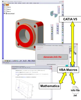
Storing these information allows a fast reclassifica-tion of the parts in case different thresholds are to be considered because more suitable for the types of meshing or simulations to be carried out. Actually, even if the chosen threshold values have been demonstrated to give quite good results on the set of considered parts, it is our believe that these thresh-olds might change according to the type of system used for meshing, therefore some learning techniques would be very useful to adjust the threshold to the specific engineering environment. Figure 10 shows the sequence of communication between Catia V5 and Mathematica.
The provided macro can be activated automatically or on user demand, on either a single model or on a set of models simultaneously. Actually, we foresee the possibility of automatically categorize a part
when it is designed, thus storing the computed info file as an accompanying document of each model, possibly in dedicated directory. The computed cate-gory information can then be used for making the simulation expert immediately aware of potential problems with the part and for supporting him to retrieve similar situations. This last capability can be supported only if all the already designed parts have been already classified, that’s why we also consider the second possibility, i.e. classification of set of parts on user request.
a) b) CATIA V5 VBA Macros Mathematica .txt info file
Figure 10 Sequence of communication between Catia and
Mathematica through VBA Macros.
In order to support designers in using the classifica-tion tool, some graphical forms have been created allowing the user to interact with the system. They give him the possibility to lunch the classification on the part under development or on all the parts in the database and to select the location of the info file generated. The location of the info file can be in an-other computer. Actually, we assume that each de-signer is operating on his/her own computer or has his/her own space on the network. Additionally, we have implemented the function that allows the re-trieval of all the parts belonging to a specific catego-ry.
Since the aim of the macro VBA is to make an auto-mated categorization on a large amount of CAD parts with no action of the designer, we made some exper-imentation to validate the accuracy of the algorithm.
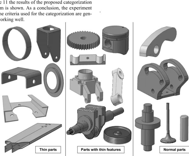
In figure 11 the results of the proposed categorization algorithm is shown. As a conclusion, the experiment is that the criteria used for the categorization are gen-erally working well.
.
Thin parts Parts with thin features Normal parts
Figure 11 Categorization of thin parts, parts with thin features and normal parts
7. CONCLUDING REMARKS AND
FU-TURE WORK
The work presented in this paper is a first step to-wards the definition of a complete toolbox for the classification of parts which are potentially complex to mesh or not. Indeed, the main aim is still how to classify parts depending on their shapes and features. With the macro and the associated algorithm, all needed information is provided to the designer and the work of evaluation of the level of complexity during meshing is done for him/her, thus he/she can focus on other issues.
The prototype has been integrated within Catia, but working directly on the computed .stl file it is made system independent and then can be easily integrated on other commercial CAD systems adopted in com-panies. Additionally the use of the info file storing all the key shape descriptors and thresholds may allow a quick different categorization of the parts according to the user/system needs, being the most time
con-suming activity related to the shape descriptor evalu-ation.
Anyhow, the approach proposed is not exhaustive and additional criteria can be created to refine the categorization.
Current work includes the optimization of the algo-rithm to improve its efficiency and overcome the limits in the classification for the limited number of complex parts which are not well-classified. There will always be parts that the algorithm will not be able to treat, thus one of the possible future extension is the inclusion of some learning capabilities for both identifying the best threshold and descriptor combi-nation.
In the future, we plan to work on returning additional information to the user on the shape elements corre-sponding to the thin areas. This would be used to-gether with the already evaluated data in helping him in suitably modify the part and in selecting the most appropriate mesh size to use.
ACKNOWLEDGMENTS
The work has been partially supported by the VI-SIONAIR project funded by the European Commis-sion under grant agreement 262044.
REFERENCES
[1] Cardone, A., Gupta, S.K. and Karnik, M. (2003) "A survey of shape similarity assessment algorithms for product design and manufacturing applications", Journal of Computing and Information Science in En-gineering, Vol. 3, No. 2, pp.109-118.
[2] Iyer, N., Jayanti, S., Lou, K., Kalyanaraman, Y. and Ramani, K. (2005) "Three-dimensional shape search-ing: state-of-the-art review and future trends", Com-puter Aided Design, Vol. 37, No. 5, pp. 509-530. [3] J.W. H. Tangelder · R. C. Veltkamp, (2008) “A
sur-vey of content based 3D shape retrieval methods”, Multimed. Tools Appl., vol. 39, pp. 441-471.
[4] Osada, R., Funkhouser, T., Chazelle, B., and Dobkin, D. (2002) “Shape distributions”, ACM Transactions on Graphics (TOG), Vol. 21, No. 4.
[5] C.-T. Chang, B. Gorissen and S. Melchior, (2011) “Fast oriented bounding box optimization on the rota-tion group SO(3;R)”, ACM Transacrota-tions on Graphics. [6] M. Bern, P. Plassman (2000), “Mesh generation”,
Handbook of Computational Geometry, Elsevier: Amsterdam, 291–332.
[7] Worlfram research, www.wolfram.com.
[8] K. Zhu, Y. San Wong, H. Tong Loh, W. Feng Lu (2012), “3D CAD model retrieval with perturbed La-placian spectra”, vol. 63, pp. 1-11.
[9] J. Bai, S. Gao, W. Tang, Y. Liu, S. Guo, (2010), “Design reuse oriented partial retrieval of CAD mod-els”, Computer-Aided Design, vol. 42, pp. 1069– 1084.
[10] J-C. Cuillière, V. François, K. Souaissa, A. Benamara, H. BelHadjSalah (2011), “Automatic comparison and remeshing applied to CAD model modification”, Computer-Aided Design, vol. 43, pp. 1545–1560.
![Figure 2 Taxonomy of shape matching methods [1].](https://thumb-eu.123doks.com/thumbv2/123doknet/7334608.211871/4.892.90.431.136.421/figure-taxonomy-shape-matching-methods.webp)