J . Fluid Mech. (1996), vol. 329, pp. 25-64 Copyright 0 1996 Cambridge University Press
25
Benard-Marangoni instability in rigid rectangular
containers
By P. C . D A U B Y A N D G. LEBON
Universitt de Liege, Institut de Physique B5, Sart Tilman, B 4000 Likge 1, Belgium e-mail: [email protected]
(Received 7 September 1994 and in revised form 5 July 1996)
Thermocapillary convection in three-dimensional rectangular finite containers with rigid lateral walls is studied. The upper surface of the fluid layer is assumed to be flat and non-deformable but is submitted to a temperature-dependent surface tension. The realistic ‘no-slip’ condition at the sidewalls makes the method of separation of variables inapplicable for the linear problem. A spectral Tau method is used to determine the critical Marangoni number and the convective pattern at the threshold as functions of the aspect ratios of the container. The influence on the critical parameters of a non-vanishing gravity and a non-zero Biot number at the upper surface is also examined. The nonlinear regime for pure Marangoni convection
(Ra = 0) and for Pr = lo4,
Bi
= 0 is studied by reducing the dynamics of the system to the dynamics of the most unstable modes of convection. Owing to the presence of rigid walls, it is shown that the convective pattern above the threshold may be quite different from that predicted by the linear approach. The theoretical predictions of the present study are in very good agreement with the experiments of Koschmieder & Prahl (1990) and agree also with most of Dijkstra’s (1995a, 3) numerical results. Important differences with the analysis of Rosenblat, Homsy & Davis (19823) on slippery walls containers are emphasized.1. Introduction
When a fluid layer is heated from below, it is well known that convection sets in after a critical temperature difference is reached between the bottom and the top of the layer. In a one-component fluid, the appearance of motion results either from gravity effects (Rayleigh-BCnard problem) or from thermocapillary phenomena (Marangoni con- vection). Since the celebrated papers by BCnard (1900), Rayleigh (1916), Pearson (1958) and Nield (1964), the problem of thermogravitational and thermocapillary instabilities has been of growing interest (see, for instance, Koschmieder 1993 or Platten & Legros 1984). In most works the fluid layer is, however, assumed to be of infinite horizontal extent. This hypothesis allows the separation of variables and the linear stability problem reduces to an eigenvalue problem for a system of ordinary differential equations in the vertical coordinate. This problem has been studied thoroughly for several different boundary conditions for both the velocity and temperature at the top and the bottom of the fluid layer. However, since experiments can only take place in finite containers, the comparison between theoretical and experimental results is not always an easy task as sidewalls play an important role in small boxes.
26 P. C. Dauby and G. Lebon
the ‘envelope formalism’ (see for instance Manneville 1990) and will not be considered here. We focus instead on instabilities in boxes with small aspect ratios. In this case, the spatial horizontal pattern of the convective cells is no longer degenerate as in infinite layers but is determined by the lateral confinement of the sidewalls.
A linear study of pure gravity-driven instability in rectangular containers with rigid horizontal and lateral walls was presented by Davis (1967). He predicted the appearance at threshold of ‘finite rolls (cells with two non-zero velocity components dependent on all three spatial variables) with axes parallel to the shorter side’. These ‘finite rolls’ have been criticized by Davies-Jones (1970) and by Luijkx & Platten (1 98 1) who considered more realistic three-dimensional solutions.
The problem of thermocapillary convection in finite boxes was first considered by Rosenblat, Davis & Homsy (1982a) and Rosenblat, Homsy & Davis (19823). These authors presented a linear and nonlinear study of thermoconvection due to temperature induced surface tension variations in circular and rectangular containers. However, their work is based on the ‘slippery’ lateral walls assumption. This boundary condition for the velocity is not realistic but enables the linear problem to be solved by using the method of separation of variables, at least for adiabatically insulated sidewalls. The nonlinear approach proposed by these authors concerns only roll-patterns but an extension was proposed by Dauby et al. (1993) who examined the possibility of the occurrence of hexagonal convective cells.
More recently Winters & Plesser (1988), van de Vooren & Dijkstra (1989) and Dijkstra (1992) have examined pure Marangoni convection with a ‘no-slip condition’ at the lateral boundaries. The velocity actually vanishes on the lateral walls and the method of separation of variables does not work. Their approaches are based on finite- element or finite-volume methods but are restricted to two-dimensional containers.
Since we submitted the first version of this work, Dijkstra has also considered Marangoni convection in three-dimensional rigid square boxes and he has obtained interesting results by using powerful numerical methods (Dijkstra 1995 a-c). The first paper (1995~) is devoted to a linear study of stability. The second is a study of nonlinear convection in square containers with aspect ratios smaller than 6. In the third work, larger-aspect-ratio containers are investigated and hexagonal convection is shown to be possible in sufficiently large vessels. The results of Dijkstra will be compared with ours and used as validation of our method.
In the present work, we study the problem of thermocapillary convection in the general case of three-dimensional rectangular containers with realistic rigid (no-slip) lateral walls (see also Dauby & Lebon 1994; Dauby, Lebon & Colinet 1996). It is assumed that the upper surface of the layer is flat and non-deformable and that the lateral walls are adiabatically insulated. We consider both linear and nonlinear analyses. The dependence of the linear results on non-zero Rayleigh and Biot numbers is also examined. In the nonlinear study, the Rayleigh and Biot numbers are fixed to 0 and the Prandtl number is equal to lo4, which is a good approximation for the silicone oils used in many experiments.
The structure of the paper is as follows. In the next section, the basic equations are given. The linear analysis of the problem is developed in 93 while the nonlinear approach is treated in 94. Conclusions are drawn in the last section. Some technical points are developed in Appendices A and B.
Bknar&Marangoni instability in rigid rectangular containers 27 2. Basic equations
The system consists of a thin viscous fluid layer filling a rectangular container. The thickness of the layer is equal to d and the length and width of the container are a, d
and a, d, respectively (a, and a, are the aspect ratios). The surface tension at the upper free surface is assumed to be temperature dependent. The fluid is heated from below. It is well known that motion sets in after the vertical temperature gradient has reached a critical value.
In the reference state, the fluid is at rest and heat propagates by conduction only: the corresponding velocity and temperature fields are given by u, = 0, T, = TB - ( A T / d ) z ; u = (u, u, w) is the velocity vector and T the temperature field; subscript r refers to the
reference state, TB is the temperature of the fluid at the bottom of the box and A T is
the temperature drop between the bottom and the top of the layer. The z-axis is vertical and oriented from the bottom to the top of the box.
The velocity perturbations u = (u, u, w) and the temperature perturbation 8 with respect to the conductive solution are governed by the Boussinesq nonlinear equations :
v-u
= 0, (2.1)- dB = w
+
V2B. dtEquations (2.1)-(2.3) are written in dimensionless form with space, time and temperature scaled by d, P l K and AT, respectively; p is the dimensionless pressure and
e, the unit vector along the z-axis. The material time derivative is denoted by dldt = a/at
+
v . V . The Rayleigh number Ra is defined bya g A T b
Ra = >
KV
where 01 is the coefficient of volumetric expansion and g the acceleration due to gravity;
v is the kinematic viscosity of the fluid and K its heat diffusivity. The Prandtl number
Pr is given by
V
Pr = -
K ’
The boundary conditions are the following.
The bottom of the box is rigid and perfectly heat conducting so that
v = B = O at z = O . (2.6) The upper surface of the fluid is assumed free, plane and non-deformable. The surface tension [ is supposed to be a linear function of the temperature:
t ( T ) = f(T,)-y(T-
GI.
(2.7)T, is a reference temperature, say the temperature of the ambient surroundings and
y = -af/aT is a constant which is positive for most fluids.
At the top of the layer, heat is transferred from the liquid to the ambient gas according to Newton’s cooling law
28 P. C. Dauby and G . Lebon
where q is the normal component of the heat flux vector at the surface of the fluid, at temperature T,;
qzt
is the constant temperature of the external medium and h the heat transfer coefficient assumed to be constant. The mathematical expressions for the boundary conditions at the upper surface are (Pearson 1958; Nield 1964; Rosenblat etal. 1982a, b)
w = O at z = 1 , (2.9)
ae
-+BiB=O
aZ
at z = 1, (2.10) (2.11) where V , =(a/ax,
a/ay) is the horizontal gradient and Ma the Marangoni numberdefined by
y A T d
Ma=-. (2.12)
P * K
The symbol Bi = hd/h stands for the non-dimensional heat transfer coefficient (the so-called Biot number), with h the heat conductivity of the fluid. In (2.12), p is the mass density.
The sidewalls are adiabatically insulated and rigid. The corresponding boundary conditions for velocity and temperature are
(2.13)
ae
u = v = w = - = O ax at x=O,a 1’ae
aY
(2.14) u = v = w = - = O at y = O a 3 2’3. Linear stability problem
The linear stability problem consists in determining the critical value of the Marangoni or Rayleigh number above which convection sets in. This is achieved by first linearizing equations (2.1k(2.3). The boundary conditions (2.6), (2.9)-(2.1 I), (2.13) and (2.14), which are linear, keep the same form. Then, an exponential time dependence of the form exp(d) for all the variables is introduced in the equations, which results in an eigenvalue problem for the Marangoni number, the Rayleigh number or the growth rate CT:
v * v = 0, (3.1)
V2v-Vp+RaOe, = Pr-lcrv, (3
4
v2e
+
w = (To. (3.3)Since we are mainly interested in surface-tension driven instability, we will consider in this section that the Rayleigh number is fixed and we will determine the critical Marangoni number characterizing marginal stability. Moreover, the principle of exchange of stability is assumed to hold. It is supposed that the growth rate of the most dangerous mode passes from real negative to real positive values as the control parameter is increased above its critical value. This assumption has been shown to be valid for pure buoyancy instability (Pellew & Southwell 1940) owing to the self- adjointness of the relevant equations. Exchange of stability was also proved numerically
Benard-Marangoni instability in rigid rectangular containers 29 to hold in the case of pure thermocapillary (Vidal & Acrivos 1966) and coupled buoyancy and thennocapillary (Takashima 1970) instabilities in infinite boxes. For finite containers, no demonstration has been proposed up to now. Nevertheless, Rosenblat et al. (1982a, b) have taken this principle for granted in the case of slippery lateral boundaries. Moreover, numerical works by Dijkstra (1992, 19953) show that no Hopf bifurcations occur at threshold in rigid containers. So the assumption of exchange of stability is made here and both the real and imaginary parts of the perturbations growth rate are assumed to vanish at the threshold.
In their papers, Rosenblat et al. use the method of separation of variables to study the linear Marangoni instability in a container with slippery walls. As shown by Pellew & Southwell (1940), this method cannot be applied when the sidewalls are rigid and a numerical resolution of the eigenvalue problem must be considered.
3.1. The numerical method
The numerical method to be used here is the so-called spectral Tau method (Canuto
et al. 1988), which is a refinement of the well-known Galerkin method (Finlayson 1972). Following this approach, the unknown fields are expanded in series of trial functions which form a complete set and satisfy some of the boundary conditions, the so-called ‘essential’ boundary conditions. Truncated series are introduced in the field equations as well as in the ‘natural’ boundary conditions which are not a priori satisfied by the trial functions. Then these equations and natural boundary conditions are projected on the same trial functions, i.e. the equations and natural boundary conditions are multiplied by the trial functions before being integrated over the fluid volume. The purpose of this procedure is to replace the set of differential equations by a set of algebraic equations.
In the present problem, the unknowns v(u, v,
w)
and 0 are written in the formwhere N,, N y and N, are integers; vck = (uCk, 0, wek), vck = (0, v : ~ , wek) and Bijk are trial functions which are specified in Appendix A; Aijk, Bijk and Cijk are unknown
constants. The total number of trial functions or degrees of freedom is thus given by 3 x N, x N y x N,.
The unknown pressure p is not given an explicit decomposition because the pressure gradient disappears in the final equations, thanks to integration by parts and boundary conditions.
The expressions vck = (uck, 0, wek,> and vck = (0, vck, wek,> correspond to the ‘finite
rolls’ solutions of Davis (1967), i.e. to modes of convection for which one of the two horizontal components of the velocity vanishes but whose non-zero components are actually functions of the three spatial coordinates. The upper indices
X
and Y definethe ‘x-rolls ’ and
‘
y-rolls ’ of Davis which are parallel to the y- and x-axes, respectively. Let us mention that these finite rolls have been criticized by different authors (Davies- Jones 1970; Luijkx & Platten 1981; Platten & Legros 1984) who showed that these modes of convection can never be exact solutions of the problem. In the present work, we do not consider separately x-rolls and y-rolls, as done by Davis, but we decompose the solution into a sum of such rolls.The precise form of the trial functions and some further details on how to obtain the algebraic eigenvalue problem are given in Appendix A. Note only that, owing to the symmetry between the ‘length’ and the ‘width’ of the box, the solutions of the eigenvalue problem may be separated into four classes which are characterized by the
30 P. C. Dauby and G . Lebon
parity of the unknown fields with respect to the coordinates x and y . The four classes will be denoted EE, EO, OE and 00. The first and second letter of each of these symbols respectively refers to the parity of the x- and y-dependences of the temperature field. Note also that the normalization condition that has been used in the determination of the algebraic eigenvectors is written as
C
lei1
= 1, (3.5)i
where 0, represents the values of the temperature field at the nine points chosen at mid- depth of the container and with x-coordinates equal to 0, -+a,, -a, and y-coordinates equal to 0, -fa,, - a,. This normalization condition is of importance for the nonlinear analysis developed in 94.
3.2. Results
Before considering three-dimensional containers, we have checked our method by comparing our two-dimensional results with previous approaches based on other techniques.
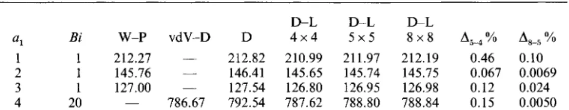
Table 1 gives a comparison with the works of Winters & Plesser (1988), van de Vooren & Dijkstra (1989) and Dijkstra (1992). The convergence of our algorithm is also examined. The agreement between the present work and the previous ones is excellent as soon as N , x N, is equal to 5 x 5. The convergence is also very satisfactory since the difference between the results with N,xN, = 8 x 8 and those with
N, x N, = 5 x 5 is always smaller than 0.10
YO.
The fast convergence with a rather small number of trial functions is one of the principal improvements of the present work for two-dimensional containers with respect to the linear approaches given by Winters & Plesser (1988), van de Vooren & Dijkstra (1989) and Dijkstra (1992). Clearly, the decomposition in terms of Chebyshev polynomials is responsible for this fast convergence.The results corresponding to the more realistic problem of three-dimensional rectangular containers are now analysed. As a preliminary, let us discuss the problem of the convergence of our method. In table 2 are found the numerical results corresponding to different values of the Rayleigh and Biot numbers and different numbers of trial functions. Two couples of aspect ratios are considered, namely
(a,, a,) = (4,2) and (a,, a,) = (6,5). It is observed that the critical parameters evaluated
with N, x N , x N , = 6 x 6 x 6 vary by less than 0.035
YO
with respect to the valuescorresponding to N , x N, x N, = 5 x 5 x 5. Therefore, the next calculations are
performed with N, x N, x N, = 5 x 5 x 5.
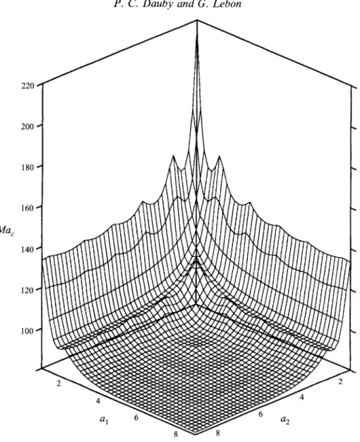
Table 3 presents the values of the critical Marangoni number for some aspect ratios and for zero Rayleigh and Biot numbers. Figure 1 is a three-dimensional picture of Ma, as a function of the aspect ratios a, and a, (Ra =
Bi
= 0). The calculations have beenperformed for aspect ratios varying by discrete steps of 0.2. The critical Marangoni number is seen to be a globally decreasing function of the lateral dimensions of the containers. When both a, and a, become greater and greater, Ma, tends to 79.607, which is the value found for an infinite box. However, if only one of the two aspect ratios becomes infinite, the other one being fixed, then the critical Marangoni number tends to a value which is greater than that for infinite boxes. A similar behaviour was found by Davis (1967) for pure gravity driven convection. It is also interesting to note that the decrease of Ma, consists of portions of concave surfaces. The intersections of these portions describe, in fact, the appearance or disappearance of convective cells, or, more precisely, these intersections correspond to the transitions from one class of parity for the eigenmode (EE, EO, OE, 00) to another.
Benard-Marangoni instability in rigid rectangular containers 31
D-L D-L D-L
a1 Bi W-P vdV-D D 4 x 4 5 x 5 8 x 8 A5-4% As-s 'Yo
1 1 212.27 - 212.82 210.99 211.97 212.19 0.46 0.10
2 1 145.76 - 146.41 145.65 145.74 145.75 0.067 0.0069
3 1 127.00 - 127.54 126.80 126.95 126.98 0.12 0.024
4 20 - 786.67 792.54 787.62 788.80 788.84 0.15 0.0050
TABLE 1. Critical Marangoni number for different aspect ratios a, and Biot numbers Bi; Ra = 0. The results of Winters & Plesser (1988) (W-P), van de Vooren & Dijkstra (1989) (vdV-D) and Dijkstra
(1992) (D) are reported in columns 3-5. The following three columns (D-L) present our results with
the different values of N, x N, indicated in the first cell. The last two columns give the differences in
per cent between columns 5 x 5 and 4 x 4 and columns 8 x 8 and 5 x 5 respectively. Note that the definition of the Marangoni number in van de Vooren & Dijkstra (1989) and Dijkstra (1992) is different from ours but the values given here have been adapted to our definition.
(a,,%) Ra Bi 4 ~ 4 x 4 5 ~ 5 x 5 6 ~ 6 x 6
(4, 2) 0 0 97.171 97.219 97.228 0.0093
(4, 2) 300 0 63.766 63.865 63.871 0.0094
(4, 2) 0 10 479.91 481.16 481.33 0.035
(6, 5 ) 0 0 83.430 83.475 83.477 0.0024
TABLE 2. Convergence of the critical Marangoni number for different values of the Rayleigh and Biot numbers. The numbers N,, N,, N, of trial functions are given in the first cell of each column. The last
column gives the differences in per cent between columns 6 x 6 x 6 and 5 x 5 x 5 .
a,\% 2 3 4 5 6 7 2 111.48 101.18 97.219 95.484 94.622 94.144 3 101.18 91.080 88.770 88.034 88.293 87.092 4 97.219 88.770 85.771 84.551 84.462 83.453 5 95.484 88.034 84.551 83.772 83.475 82.484 6 94.622 88.293 84.462 83.475 83.178 82.184 7 94.144 87.092 83.453 82.484 82.184 81.976
TABLE 3. Values of the critical Marangoni number for different aspect ratios and for Ra = Bi = 0 ( N , x N , x N, = 5 x 5 x 5).
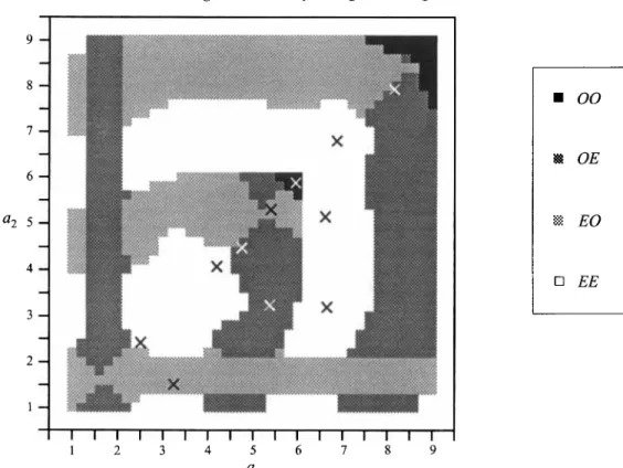
The study of the number and the form of the convection cells is performed by using figure 2. This picture is a map of the modes of convection at threshold: to each pair of aspect ratios (a,,a,) is associated a small square whose relative darkness is determined by the class 00, OE, EO or EE to which the critical solution pertains.
Clearly, the instability is degenerate for boxes whose aspect ratios are located on the intersection of zones of different darkness since, in this case, several distinct convective modes become simultaneously unstable. The linear results for square containers are presented in figure 3. The different portions of the decreasing Ma, function are clearly exhibited as well as the mode switching. Note that not only the smallest eigenvalue Ma, has been plotted, but also some other curves corresponding to the successive eigenvalues.
A precise interpretation of the map of convective patterns at threshold (figure 2) is not completely straightforward and requires the explicit representation of the convective cells for at least some values of the aspect ratios. As an example, let us
32 P. C. Dauby and G. Lebon 220 200 180 160 Mac 140 120 100
FIGURE 1. Critical Marangoni number as a function of the aspect ratios for Ra = Bi = 0.
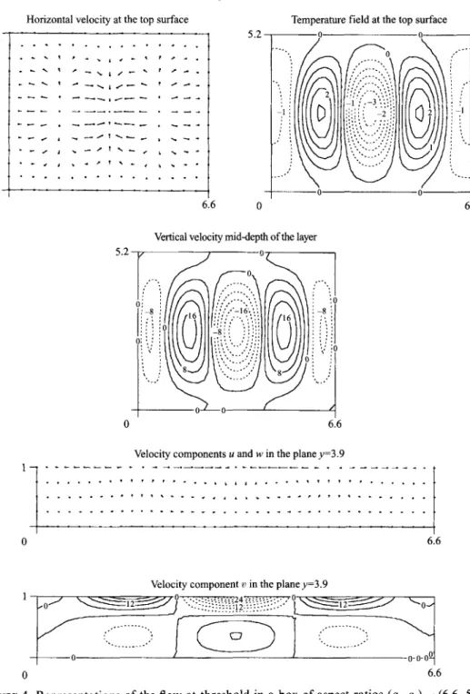
consider a container with (a,,a,) = (6.6, 5.2) in the case of zero Rayleigh and Biot numbers. For this container, the solution belongs to the EE class as shown in figure 2. Various features of the flow in this box at threshold are found in figure 4. We show the horizontal velocity vector and the temperature field at the top surface and also the vertical velocity u’ at mid-depth of the layer. We then show the velocity components u and w in the vertical plane y = 3.9 as well as the velocity component u in this plane. It is clearly seen that convection sets in in the form of four rolls with axes parallel to the shorter sides of the container.
To analyse figure 2, note first that this picture is ‘symmetric’ with respect to the line
a, = a, and only the region with a,
<
a2 will be studied in detail. Furthermore, figure 2 is seen to be made up of different strips with distinct colours. We will now see that each strip corresponds to a flow pattern taking the form of convective rolls which are usually parallel to the shorter sides of the box. For square boxes, rolls parallel to both sides may possibly combine to produce a more symmetric structure.Bknard-Marangoni instability in rigid rectangular containers 33
1 2 3 4 5 6 7 8 9
a1
FIGURE 2. Map of the convective modes at threshold for Ra = Bi = 0. Crosses indicate boxes which are considered in detail in the nonlinear analysis ($4.4).
2 3 4 5 6 I 8 9
a1
FIGURE 3. Critical Marangoni number as a function of the aspect ratio for square boxes
(Ra = Bi = 0). The curves corresponding to several successive eigenvalues are also plotted and the parity of the eigenmodes is indicated.
34 P. C. Dauby and G. Lebon
. . .
. . .
. . .
0 5.2Temperature field at the top surface
5.2-0
I
t
6.6 0
Vertical velocity mid-depth of the layer
0 6.6
6 6
Velocity component w in the plane y=3.9
..:
7 .__. - ..__.
0 ...
I 0- 0- 00
0 6.6
FIGURE 4. Representations of the flow at threshold in a box of aspect ratios (ul, a,) = (6.6, 5.2). The Rayleigh and Biot numbers are zero.
First, we consider boxes for which the aspect ratios are ‘quite’ different; the case of square or quasi-square containers will be studied later on. From figure 4 and from representations of the flow for other boxes with aspect ratios in the same EE zone, it
may be inferred that the white strip in the neighbourhood of a, = 6.2 in figure 2
corresponds to a convective structure in the form of four rolls parallel to the shorter sides of the container. Similarly, the dark grey strip centred on a, = 4.8 and the white
B&nard-Marangoni instability in rigid rectangular containers
(4
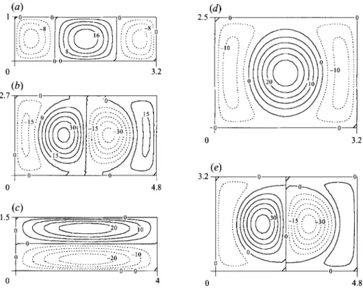
3.2 0 0-4 3.2 35 0 4 0 4.8FIGURE 5. Representation of the flow at threshold for several rectangular containers (Ra = Bi = 0). The iso-values of the vertical velocity w at mid-depth of the fluid layer are represented. The aspect ratios are: (a) (3.2, l), (b) (4.8, 2.7), ( c ) (4.0, lS), (d) (3.2, 2.5), (e) (4.8, 3.2).
strip centred on a, = 3.2 describe, respectively three (figures 5b and 5e) and two (figures 5a and 5 d ) rolls parallel to y. There are also five rolls near a, = 8.2. The horizontal light grey zone with a, = 1.6 corresponds to a unique convective roll parallel
to the x-axis (figure 5c), that is parallel to the larger sides of the box, and in the small light grey area near ( a , , ~ , ) = (5.6, 5.2), convection sets in in the form of three rolls parallel to the larger sides of the container.
In square containers, the convective structures are the following. For very small cavities (a,
<
2.2), a degenerate solution is found in which one roll parallel to yand one roll parallel to
x
become simultaneously unstable at threshold. For a, = 2.5 (EE zone), a unique square cell is observed (figure 6a). For a, = 4.4, there is also a square cell (figure 6b) but the picture is somewhat different from figure 6(a). As a matter of fact, a cell similar to that corresponding to a, = 2.6, but rotated by 45", isseen in the middle of figure 6(b) and the flow in the corners of the box is very weak. In connection with these pictures, it is interesting to wonder how square cells can be built in infinite layers. As recalled by Koschmieder (1993), the
(x,
y)-dependence of the vertical velocity in square cells can be written either as the sum (w = (coskx+
cos ky) W(z)) or as the product ( w = cos 2-1/2kx
cos 2-l" ky W(z)) of the functions ofx
and y which define the vertical velocities corresponding to two sets of perpendicular rolls. Figure 6(a) is made up by the sum of two rolls perpendicular tox
and two rolls perpendicular to y while figure 6(b) represents, rather, the product of such rolls. In both cases, the rolls parallel to both sides combine to give rise to a symmetric structure. For larger boxes (dark and light grey areas near a, = 4.8), the instability is degenerate and either three rolls perpendicular to x or three rolls36 P. C. Dauby and G . Lebon 2.5 0 (a> ... ... ... ... I L 2
(4
I 0 O l 4.1 " " I 4.1 -0 ... -0- ... ... .... ... ... ... 1 ... L L 4.4 0 5.9 4.4 8 - c.- 0 O - 1 ro 9 0 8 FIGURE 6. Representation of the flow at threshold for several square containers (Ra = Bi = 0). The iso-values of the vertical velocity w at mid-depth of the fluid layer are represented. The aspect ratios are: (a) 2.5, (b) 4.4, (c) 4.7, ( d ) 5.9, (e) 6.8,cf>
8.0.Bknard-Marangoni instability in rigid rectangular containers 37
perpendicular to y appear (figure 6c). The pattern for the black 00 zone in the neighbourhood of a, = 5.9 is given in figure 6 ( d ) and presents an 'antisymmetric'
structure, which could be seen as the 'product ' of three rolls parallel to x and three rolls parallel toy. In the white area in the vicinity of a, = 6.2, the convective structure (figure 6 e ) consists of one square cell (similar to figure 6a, with opposite sign) in the middle
of the box but a ring of sinking fluid is also observed along the sidewalls. For still larger values of the aspect ratio (light and dark grey zones near a, = 8), one observes five rolls parallel to any side of the container (figure 6 8 . For quasi-square containers, the convective cells are similar to these which appear in the square cavities but slight deformations are observed.
The degeneracy of the instability in square boxes may be related to the symmetry of the convective patterns. For EE solutions (figures 6a, 6 b and 6e), the convective structure is clearly invariant for a reflection about the medians of the box and also for a rotation of 90" around the centre of the container. Similarly, the 00 solutions (figure
6 d ) have the same symmetry since the linear convective pattern is defined to within a
change of sign. In both cases, the instability is non-degenerate and the critical eigenvalue is simple. On the other hand, when the eigenvector is an element of the EO or OE class, the structure is still invariant for the reflections with respect to the medians but the invariance is lost for a rotation of 90" of the pattern. In fact, for square containers, the EO or OE modes are simultaneously unstable and the EO pattern may be obtained by rotating the OE one by 90", and vice versa. In the light and dark grey zones of figure 2, the instability is degenerate and the eigenvalue has an algebraic multiplicity equal to 2.
A tentative physical interpretation of the geometrical nature of the convective cells at threshold in rectangular containers may be the following. The selection of the convective pattern is based on a balance between two arguments. The first one put forward by Davis (1967) and also taken up by Koschmieder (1993) states that, owing to dissipation at the rigid walls, a structure with rolls parallel to the shorter sides of the container dissipates less kinetic energy than a structure consisting of rolls parallel to the longer sides of the box. For this reason (Chandrasekhar 1961), the pattern with rolls parallel to the shorter sides is more likely to appear in experiments. The second argument which enables us to explain our results is the fact that the system prefers a structure for which the rolls are not compressed too much or dilated but have a dimension more or less equal to the dimension they would have in an infinite layer. For zero Biot and Rayleigh numbers, the critical wavenumber in infinite layers is about 2 and the width of the rolls is more or less equal to 1.6. Consider for instance a box with
(a,,a,) = (5, 3.2). This box may be filled up with three rolls parallel to y or with two
rolls parallel to x. In both cases, the width of the rolls is about the 'optimal' value 1.6. The argument of dissipation along the walls will then impose the structure with three rolls parallel to the shorter sides of the container. In a box with (al, a,) = (5.7,5.2), three
rolls parallel to the larger sides of the container can be observed because the rolls parallel to y would not present an optimal width. All the results represented in figure
2 may be explained by using these two arguments. Of course, for large values of the aspect ratios, the argument about the width of the rolls becomes less relevant since the box can always be filled up with rolls of nearly optimal dimension. For this reason, the areas describing rolls parallel to the longer sides of the containers tend to disappear in large enough vessels. Let us also add that rolls parallel to each side may combine to form square or quasi-square cells in the neighbourhood of the diagonal a, = a,.
At this stage, it is interesting to compare our results with those of Dijkstra (1995a). Although both results are quite similar, our calculations are a bit more precise. For
38 P. C. Dauby and G. Lebon
instance, in a square box with aspect ratio 4, Dijkstra gets the value 86.27 for the critical Marangoni number by using about 5 x 163 z 2 x lo4 degrees of freedom (see Dijkstra’s table 1). With N , = N , = N , = 5 (number of degrees of freedom =
3 x N , x N , x N, = 3 x 53 = 379, we obtain Ma, = 85.771. This value is highly reliable since for (Nz, N u , N,) equal, respectively, to (6, 6, 4), (7, 7, 5), and (8, 8, 6), we found the values 85.718, 85.771 and 85.775. This small lack of precision in Dijkstra’s approach has no influence in small boxes where the successive eigenmodes bifurcate far from each other, but becomes important in larger boxes. For instance, Dijkstra missed the small 00 areas of figure 2 and the pattern presented in his figure 3(g) does not correspond to the first linearly unstable eigenmode; the most unstable mode looks like our figure 6(d).
We would also like to mention that some patterns given by Dijkstra (1995a) are in fact not so different from one another as they may appear at first glance. For instance, his figures 3 (d)-3
(f)
(boxes of aspect ratios 4.5, 5 and 5.5) correspond in our work to degenerate eigenmodes of classes EO and OE and the unique convective structure looks like our figure 6(c) (box of aspect ratio equal to 4.7; three convective rolls parallel to any side of the container). We think that Dijkstra’s pictures look different from one another and also from our figure 6(c) because they are in fact some superposition of the two eigenmodes EO and OE.We now compare our work with the celebrated paper by Rosenblat et al. (19826) who used the simplified boundary condition of slippery lateral walls. First of all, note that, with realistic no-slip lateral walls, the critical Marangoni number is systematically larger than the value 79.607 characterizing the instability in non-bounded domains. In the paper of Rosenblat et al. (1982b), this value 79.607 was found for many finite boxes, which is not physically realistic.
It is also interesting to compare our map of critical modes (figure 2) with the corresponding result of Rosenblat et al. (19826) (see their figure 7). Although the two pictures look quite different, some interesting similarities emerge. Actually, the different strips corresponding to a fixed number of rolls also appear in the picture of Rosenblat et al., although if the borders of their ‘strips’ are more jagged. Indeed, the critical mode in containers with a, z irnn (or a2 z inn) is always the mode (m, 0) (or the mode (0,n)) and this mode consists of m rolls parallel to y (or n rolls parallel to x). However, a difference exists between rigid and slippery walls because the strips corresponding to rolls parallel to the longer sides of the box do not disappear in large slippery boxes. This result is not surprising because, as in rigid boxes, the rolls always try to have an optimal width if the sidewalls are assumed slippery. However, in this case, no energy is dissipated along the walls and the rolls can therefore be found parallel to any border.
Another difference between both kinds of containers is that, in figure 7 of Rosenblat
et al., some intermediate regions exist between the strips corresponding to pure rolls. Moreover, within each particular domain of their figure 7, the convective pattern is always self-similar and the only modification of the pattern within one domain is some dilation or contraction. In our figure 2, the different strips are contiguous and the convective pattern varies continuously within each strip.
The influence of non-zero Rayleigh and Biot numbers has also been considered in our analysis. In particular, the linear approach of the stability problem has been carried out for R a = 300, Bi = 0 and for Ra = 0,
Bi
= 10. As expected, an increase of R acorresponds to a decrease of the critical Marangoni number. Another relevant result is the fact that the map of the modes of convection obtained for a non-zero Rayleigh number is nearly completely similar to that of figure 2. This means that gravity has
Bknard-Marangoni instability in rigid rectangular containers 39 nearly no influence on the selection of the linear convective pattern. In the case of infinite layers, a corresponding result is well known (Nield 1964; Lebon & Perez- Garcia 1980) since the critical wavenumber is nearly independent of the Rayleigh number. One has also observed that by increasing the Biot number, the critical Marangoni number grows. The map describing the convective patterns for Bi = 10 is also very similar to that for Bi = 0 (figure 2) but with the important restriction that the transitions between the different zones occur for smaller values of the aspect ratios : the map for Bi = 10 can be drawn by ‘compressing’ along both axes the map given in
figure 2. This result may be related with the fact that, in infinite layers, the critical wavenumber decreases if Bi is increased (Nield 1964; Lebon & Perez-Garcia 1980). A physical interpretation of this tendency was proposed by Nield (1964): when Bi is not zero, a larger temperature gradient is necessary to cause instability. More energy must be dissipated and smaller cells appear.
4. Nonlinear Marangoni convection
4.1. The method of resolution
To account for the evolution of the convective pattern above threshold, we follow a method first introduced by Eckhaus (1965). The same technique was used by Rosenblat
et al. (1982a, b) in their nonlinear approach to Marangoni convection in slippery boxes and by Parmentier et al. (1996) in the case of horizontally infinite boxes. Some general considerations on this nonlinear approach to convection may be found, for instance, in Manneville (1990). Note also that the adjoint linear eigenvalue problem is required to apply the method. For completeness, this adjoint problem is given in Appendix B. The method consists first in expanding the solution of the nonlinear equations in series of the eigenmodes of the linear problem. The time-dependent coefficients are the so-called ‘amplitudes’ of the different modes of convection. The eigenmodes to be used here are the eigenmodes of set (3.1k(3.3) considered as an eigenvalue problem for the growth rate cr, when the Marangoni number is fixed and equal to Ma,. Clearly the smallest eigenvalue of this problem is zero and corresponds to the marginally stable convective mode. If the eigenmodes are assumed to form a complete set, one may write :
where A,(t) are the amplitudes and (up, 8,) denote the eigenmodes (of any parity EE,
EO, OE or 00) of the linear eigenvalue problem for cr with Ma = Ma,. All the boundary conditions, except the Marangoni conditions at the upper surface, are automatically fulfilled if the unknown fields take the form (4.1). Moreover, the continuity equation (2.1) is also directly satisfied. The Marangoni conditions can, however, be taken into account by slightly modifying expression (4.1): indeed, the continuity equation and all the boundary conditions are satisfied by:
Note that, for the forthcoming developments, it is worth assuming that the eigenmodes are ordered by decreasing growth rate
CT,
: upd
CT* 6 0 if p>
q.Introduce then this development (4.2) in the nonlinear equations (2.2k(2.3) for the velocity and temperature. Multiply (2.2) by u: and (2.3) by (Ma/Ma,)O$, where
40 P. C. Dauby and G. Lebon
(u;, 0;) denotes an eigenmode, with eigenvalue CT,, of the adjoint eigenvalue problem (B 1)-(B 8) considered as an eigenvalue problem for the growth rate when Mu = Ma,.
Add both expressions and integrate over the fluid volume. After performing integrations by parts and using the boundary conditions and the bi-orthogonality relations (B 9), one obtains the following evolution equations for the amplitudes A,(t):
In this expression, e is the relative distance to threshold. It is defined as
Ma - Ma,
e =
Mac
.
The matrices in
(4.3)
are given by(4.3)
(4.4)
The set (4.3) forms an infinite dimensional system of nonlinear ordinary differential equations for the amplitudes of the eigenmodes and is the basis of our nonlinear analysis.
4.2. Reduction of the dynamics in the weakly nonlinear regime
To be tractable, the infinite dimensional set
(4.3)
must be simplified and, in particular, it must be restricted to a finite number of equations. The use of a finite number of equations can be justified by noting that, in the weakly nonlinear regime, only a small number of eigenmodes are linearly unstable while all other modes have negative growth rates. It is convenient to share out the eigenmodes into two sets. The first set contains the ‘unstable’ eigenmodes which bifurcate in the vicinity of the threshold and which are thus actually unstable in the neighbourhood of e = 0. The e-value definingthe bifurcation of the successive eigenmodes is easily obtained from
(4.3).
It is given bywhere ep denotes the value of e at which the eigenmode p bifurcates. The ‘unstable’ eigenmodes are defined by an index running from 1 to some number N , which must be determined.
The second set of eigenmodes is made up by the ‘stable’ eigenmodes whose linear growth rate remains negative in the weakly nonlinear regime. In the weakly nonlinear regime, this growth rate is given by
These stable eigenmodes do not really participate in the dynamics of the system but they cannot be omitted since they represent the nonlinear response of the system to the growth of the unstable modes. These modes are generated by the quadratic interactions of the first unstable modes and their amplitude should be expressed as a quadratic expression in the amplitudes of the unstable modes. To be more explicit, equations (4.3) for the stable modes will be simplified in the following way. First, the term proportional to e in (4.3) may be disregarded with respect to
.-,
A , since e remains small in the weakly nonlinear regime and.-,
is quite negative for a well-dampedBknard-Marangoni instability in rigid rectangular containers 41 eigenmode. Secondly, the time derivative of the amplitude is neglected since the stable modes do not participate in the dynamics of the system. Finally, the quadratic term may be restricted to a quadratic expression containing only the amplitudes of the unstable modes because, in the neighbourhood of threshold, the amplitudes of the unstable modes remain rather small and terms of order higher than 2 in these amplitudes may be neglected. The amplitudes of the stable modes can thus be written as :
In (4.9), and subsequently, indices si denote stable modes while indices ui refer to unstable eigenmodes.
Formula (4.9) shows also that the amplitudes ASi become smaller and smaller as index si increases since the corresponding growth rates become more and more
negative. In particular, eigenmodes with sufficiently negative growth rate may be disregarded since their amplitude becomes negligibly small. In practice, the contributions of the stable modes will only be taken into account for si larger than Nu
but smaller than Nu
+
N,, for some integer N , which must also be evaluated.By introducing (4.9) with N u
<
si 6 N u+
N , in (4.3), we obtain the final equations :+
c
Tl(ui, u j , u k ) A,5 A,k+
c
K(ui?
u j , uk, uL) A ~ j A u k (4' lo)u5. uk(unst) u j , ub, uz(unst)
with ui = 1,
...,
Nu. Note that, in (4.10), we have neglected terms proportional to €Au1 Auj and terms of order higher than 3 in the amplitudes of the unstable modes. The matrixT,
is given by:The above reduction of the dynamics of the system to a finite number of ordinary differential equations for the most unstable modes is the well-known adiabatic elimination of the slaved modes. The procedure has been widely developed in earlier works (see, for instance, Manneville 1990; Haken 1983; Rosenblat et al. 1982a,b; Foias et al. 1988) and will not be discussed further. It will now be applied to the study of Marangoni convection in no-slip rectangular vessels. Note that the values of the (numerous) coefficients T,, and
T,
will not be given explicitly in the paper. However, these numbers could be provided on request to interested parties.4.3. Nonlinear Marangoni convection in rigid containers
The application of the above method of reduction requires first the determination of the numbers N u and N , of the unstable and stable modes.
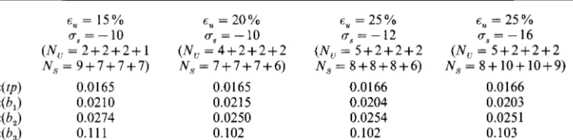
First, let us stress that we have basically in mind the determination of the bifurcation diagrams in the weakly nonlinear regime. Therefore, Nu and N , will be selected in order to provide a good description of the stable (i.e. observable) branches of the bifurcation diagrams in a range of e-values less than about 15 %. For these values of
42 P. C. Dauby and G . Lebon E, = 15% us = - 10 E, as = = 20% - 10 (Nu = 2 + 2 + 2 + 1 N , = 9 + 7 + 7 + 7 ) ( N , N , = = 7 + 7 + 7 + 6 ) 4 + 2 + 2 + 2 4 t P ) 0.0165 0.0165 4 b J 0.0210 0.0215 db,) 0.0274 0.0250 E(b,) 0.111 0.102 E, = 25% ( N , = 5 + 2 + 2 + 2 N , = 8 + 8 + 8 + 6 ) 0.0166 0.0204 0.0254 0.102 a8 = - 12 B, = 25% (Nu = 5 + 2 + 2 + 2 N , = 8+10+10+9) 0.0166 0.0203 0.0251 0.103 = - 16
TABLE 4. Positions of tp, b,, b, and b, in the bifurcation diagram corresponding to (ul, a,) = (4.7,4.6) (see figure 8) as functions of e, and a,; these parameters are defined by the fact that the ‘unstable’ modes bifurcate for B < 6, and that the ‘stable’ modes taken into account have a growth rate CT > us.
The values of N , and N , are written as sums of four numbers which give the numbers of eigenmodes
of parity EE, EO, OE and 00.
the relative distance to threshold and for
Bi
= 0, Pr = lo4, we have checked that the stable branches of the bifurcation diagrams were properly described by choosing the stable and unstable eigenmodes in the following way. First, the unstable modes are these which bifurcate for a-values less than 25YO
(and also those modes whose growth rates are less negative than the growth rates of the modes which bifurcate beforet‘ = 25 YO ; an example of such a mode is the mode for which the velocity vanishes and the temperature is a function of z only: this mode never bifurcates and its growth rate is equal to
-$’
(Parmentier et al. 1996)). Secondly, the stable modes are the modes with index higher than N u and growth rate higher than the value - 12. Of course thevalues of Nu and N , determined using these conditions depend on the aspect ratios of the container. It is also worth stressing that the eigenmodes with growth rates larger than - 12 are correctly approximated by (3.4) for boxes with aspect ratios less than about 7 if the number of trial functions is fixed by (N,,N,,N,) = (7, 7, 5). Note also
that, before considering three-dimensional situations, we have checked the validity of the method by comparing with the results obtained by Dijkstra (1992) for two- dimensional containers: the agreement was found to be very good. For three- dimensional containers, the convergence of the procedure when N , and N , are increased has been checked in the following way. First of all, we have searched for a qualitative convergence of the bifurcation diagram, that is, we have checked that the number and the kind (EE, EO, OE or 00) of the stable branches appearing for e less than about 15 YO were not changed if Nu and/or N , were increased. Secondly, quantitative information about the convergence may also be obtained by computing the positions of some secondary bifurcation points for different values of N u and N,. The results for a box of aspect ratio ( a , , ~ , ) = (4.7, 4.6) are reported in table 4. The positions of the turning point tp and the secondary bifurcation points b,, b, and b, (see
figure 8) are given for different values of N , and N,. The table shows that choosing the unstable and stable modes as explained above gives a good approximation of the bifurcation diagram.
We now examine the results corresponding to a representative sample of boxes with aspect ratios smaller than 8. The selected boxes are indicated with crosses in figure 2. The Biot number is fixed to 0 and the Prandtl number is equal to lo4. In order to avoid the degeneracy of the EO and OE modes in square geometries we study in the first
subsection the case of quasi-square containers. These quasi-square containers are also more realistic from an experimental point of view since a perfectly square geometry can never be achieved in practice.
Bknard-Marangoni instability in rigid rectangular containers 0.3 - . ... ... - ... ..-. .: '.., .._ 0 -0.1 I I I I I I I 43 0.04 - OE __.- 0.02 - . . . - ... 0 (. - ... . . . .... - .._ ... -0.02 - -0.04 I I I I I I I 3 4.3.1, Quasi-square containers
(a) Quasi-square container with aspect ratios (al, a,) = (2.5, 2.4)
The critical Marangoni number for (al, a,) = (2.5,2.4) is given by Ma, = 106.07 and the critical solution belongs to the EE class. In such a box, two modes with parity EE, one EO-mode, one OE-mode and one 00-mode bifurcate before e = 25
YO,
so that Nuis equal to 5. For conciseness and to recall the repartition between the four parity classes, we will write N , = 2 + 1
+
1+
1. With the same notation, one has N , = 2 + 2 + 2 + 2 . The final system describing the weakly nonlinear regime consiststhus in five cubic 0.d.e. for the amplitudes of the five unstable modes. This set of equations will not be written explicitly but we shall determine the corresponding bifurcation diagram. The latter is obtained by using standard continuation techniques as described for instance in Seydel(l988). A complete bifurcation diagram should give the amplitudes of all the unstable modes as functions of the distance to the threshold. However, it is sufficient for our discussion to represent only the amplitude of the most unstable mode of each parity. Moreover, it would not be useful to represent all the unstable branches since they would make the pictures very intricate and also because these branches correspond to solutions which are not experimentally observable. In the graphs, we will use solid curves to represent stable solutions and dashed lines for unstable ones. The diagrams are also extrapolated to values of e a bit larger than 15 YO.
Note, finally, that if some amplitude remains always equal to zero, its representation as a function of e is not given.
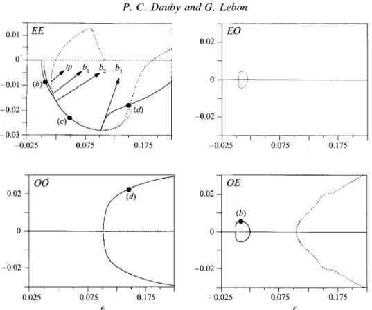
The bifurcation diagram for a box of aspect ratios (a,,a,) = (2.5, 2.4) is given in
figure 7. At the threshold, a transcritical bifurcation towards a solution made up by EE modes only can be observed. The width of the subcritical domain is equal to about 8.3
YO.
At e = 2.7YO,
there is a secondary bifurcation of the OE mode. In a progressive heating experiment, the real finite-amplitude perturbations make the system jump on the stable positive EE branch before reaching the threshold. For this solution, the motion sets in taking the form of a square cell in which the fluid rises at the centre. The convective pattern corresponding to point (a) in the bifurcation diagram is represented in figure 12(a). The structure corresponding to negative values of the EE amplitude and non-zero OE mode is not drawn because, in a progressive heating experiment, only the positive EE branch will be observed and also because the range of e for which these solutions are stable is rather small.In the same EE area of figure 2, we have also considered the box with (al, a,) = (4.2, 4.1). We found a bifurcation diagram quite similar to that given in figure 7. However,
44 P. C. Dauby and G . Lebon -0.025 ' 0.075
1
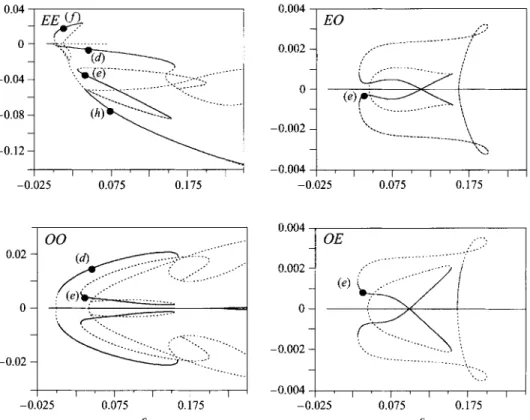
-0.02 I ' I ' I l l ' I r -0.025 0.075 0.175 & EFIGURE 8. Bifurcation diagram for a quasi-square box of aspect ratios (ul, a,) = (4.7, 4.6).
the convective pattern observed in a progressive heating experiment is different since one observes a unique square cell which is rotated by 45
YO
with respect to the cell given in figure 12(a). This kind of convective pattern also appears in the box described hereinafter and a picture of the motion in this box is given in figure 12(c).(b) Quasi-square container with aspect ratios (al, a,) = (4.7, 4.6)
In the present example, the instability is nearly degenerate. The OE mode bifurcates first but the EO solution becomes unstable quite near the threshold. The numbers of unstable and stable modes are Nu = 5+2+2+2 and N , = 8+8+8+6. The
bifurcation diagram is given in figure 8. At the threshold, one has a subcritical bifurcation towards the OE mode but the subcritical domain is very small. The EE modes are non-zero for this solution, since they are generated by the quadratic self- interaction of the OE mode. The pattern corresponding to this branch (point b: E = 1.8
YO)
is represented in figure 12(b). One main cell appears which is not located atthe centre of the container. Two other small areas of weak upflow also appear in the left-hand corners of the box. This picture corresponds to a positive value of the amplitude of the first OE mode. A negative value of the OE-amplitude would produce a pattern which is the reflection of figure 12(b) with respect to x = +a1. It is important to note that this convective structure is quite different from that found from the linear approach (see figure 6c). This is due to the presence of the EE modes which are generated by the nonlinear evolution of the OE mode. The branch corresponding to
this solutions ends up at a secondary bifurcation point on the branch originating from the bifurcation of the EE solution. At this point, the EE solution becomes stable and the observable pattern takes the form of a unique square cell with upflow in the centre.
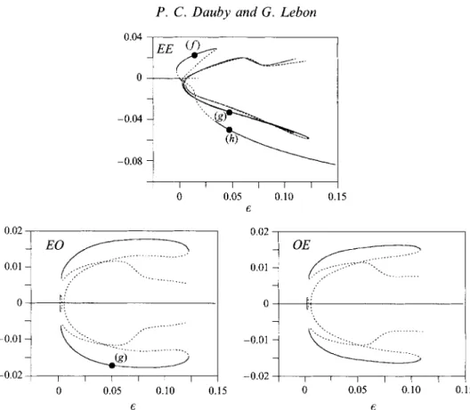
Be'nard-Marangoni instability in rigid rectangular containers 0.04 - - 0 - - -0.04 - - -0.08 - - -0.12 - 45 - -0.004 ...- ...___._ -.-.._.: ,, .... . . . ._ . . .... I ' I ' I ' I ' I I l ' l ' l ' l ' l ~ l ' -0.025 0.075 0.175 I -0.025 0.075 0.175 E -0.004
1
--0.025 0.075 0.175FIGURE 9. Bifurcation diagram for a quasi-square box of aspect ratios (ul, a,) = (5.94, 5.9).
This cell is represented in figure 12(c) for point (c) in the diagram. For larger values of E , one observes another secondary bifurcation towards a solution made up by the superposition of the EE and 00 modes (point (d)). On this branch, the convective
pattern consists of two triangular cells with upflow at the centre of each cell. A picture of the structure is given in figure 12(d). This picture corresponds in fact to a box of aspect ratios (a,,a,) = (5.94, 5.95) in which such triangular cells also appear. In the
bifurcation diagram, we have represented the (unstable) branch which arises at the bifurcation of the EO mode in order to show the quasi-degeneracy of the instability. We have also studied a slightly larger container in the same EO-OE domain. For
(al, a,) = (5.4, 5.3), the bifurcation diagram presents the following general features. At threshold, the EO mode bifurcates subcritically to give a stable structure similar to figure 12(b) but rotated by 90". The OE mode bifurcates also subcritically quite near the threshold and gives rise to a pattern similar to figure 12(b). These EO or OE solutions do, however, not exist for large value of 6. For a distance to the threshold in
the neighbourhood of 10 %, a four-square-cells solution, a two-triangular-cells pattern and a three-convective-cells structure coexist (figures 12d-12f). These three kinds of convective structures are also present in larger boxes and will be discussed in more detail later on.
(c) Quasi-square container with aspect ratios (al, a,) = (5.94, 5.9)
In figure 2, the point (a,,a,) = (5.94, 5.9) is in a black area where the 00 mode becomes first unstable. The bifurcation diagram for this container is given in figure 9
(Nu = 7
+
5+
5+
5 and N , = 12+
1 1+
1 1+
8). The bifurcation at threshold is subcritical with a very narrow domain of (unstable) subcritical convection. The EE46 P. C. Dauby and G. Lebon 0.04 0 -0.04 -0.08 I I I I I I I 0 0.05 0.10 0.15 € 0.02 0.02 0.01 0.01 0 0 -0.01 -0.01 -0.02 -0.02 0 0.05 0.10 0.15 0 0.05 0.10 0.15 € 6
FIGURE 10. Bifurcation diagram for a quasi-square box of aspect ratios (ul, a,) = (6.9, 6.8).
mode bifurcates very near threshold and, actually, the only non-conductive solution at
c = 0 is the EE mode. This branch (point
f)
corresponds to a square cell with upflowat the centre and a narrow band of rising fluid along the sidewalls (see figure 12cf) for a similar convective pattern). The 00 branch originating at the threshold becomes stable for a positive but very small value of e. The convective pattern for point ( d ) on
this branch is given in figure 12(d) and consists of two triangular cells with upflow at the centre of each cell. This structure results from the superposition of the unstable 00 mode and the EE and 00 modes generated in the nonlinear regime. Figure 12(d) corresponds to a positive value of the amplitude of the first 00 mode. A negative value for this amplitude would give a similar structure but rotated by 90". Consider now the 'negative part' of the EE branch. This branch becomes stable for c = 4.2%. The
convective pattern for this stable branch is made up by four square cells similar to the configuration observed in figure 12(a). The pattern for point H is similar to that given
in figure 12(h) which corresponds to a square box of aspect ratio 6.8. Another stable branch is also present in the bifurcation diagram. On this branch, modes of all parities are non-zero and the structure is the superposition of EE, EO, OE and 00 modes. In
figure 12(e) is plotted the convective structure corresponding to point (e) in the bifurcation diagram. Three convective cells are clearly distinguished with one square cell in the lower left-hand corner and two other wedge-shaped cells. Of course, the square cell could also be found in other corners (the 00 amplitude may take both signs and, for each sign, the EO and OE amplitudes may also be positive or negative).
Bknard-Marangoni instability in rigid rectangular containers 47 0.04
j
I._
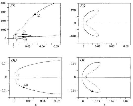
. . . I I I I I I I I I 0 0.03 0.06 0.09 I 0 I I I 0.03 I I I 0.06 I I I 0.09 I I I I I I I I I I I I I 0 0.03 0.06 0.09 6 0 0.03 0.06 0.09 6FIGURE 11. Bifurcation diagram for a quasi-square box of aspect ratios ( a , , ~ , ) = (8.1, 8).
( d ) Quasi-square container with aspect ratios (al, az) = (6.9, 6.8)
The critical eigenmode has parity EE for (a,,a,) = (6.9, 6.8). The numbers of
eigenmodes to take into account are N u = 9 + 8 + 8 + 6 and N , = 13+13+13+13.
The bifurcation diagram is plotted in figure 10. The bifurcation at threshold is transcritical with a 0.29 % width subcritical domain. Near c = 0, the negative part of
the first EE branch is stable but soon becomes unstable owing to the secondary
bifurcations of the EO and OE modes. These stable solutions exist only in very narrow
windows of 6 and could thus not easily be observed. Therefore, the convective structure is not represented. When the fluid layer is progressively heated, the system jumps onto the stable positive EE branch before reaching threshold. On this branch, the convective
pattern for point (,f) takes the form given by figure 1 2 0 : a square cell with upflow at the centre and a narrow band of rising fluid along the sidewalls. This solution becomes unstable for 6 = 3.5%and the system must jump onto another branch. For e > 3.4%, the negative EE branch becomes stable and the convection takes the form
of four square cells (see figure 12(h) for point h). Note also that this branch is the only stable solution for sufficiently large values of e. Other stable solutions are also possible. These take the form of either a superposition of EO and EE modes or a superposition
of OE and EE modes. The pattern corresponding to point (g) in the bifurcation
diagram consists of a three-cell solution as shown in figure 12(g). The three cells are, however, differently arranged to those in figure 12(e). The pattern corresponding to a positive value of the EO mode can be obtained by a reflection of figure 12(g) about
y = fa,. Similarly, the OE-EE solutions are obtained by rotating by 90" in both
48
P.
C. Dauby and G . Lebon2.4
0 (a) € = l o % 2.4
[Approximate pattern for (4.2,4.1)]
... ... 0 : .02. ... ... ...
,?
i’
... ~ . , ... ’.. -0 2. .... ... 0 (c) E =5 Yo 4.7[Approximate pattern for (5.4,5.3)]
5.9
7
...0 (e)e=4% 5.94
4.6 [Approximate pattern for (5.4,5.3)]
0 (b) E = 1.8% 4.7
5.9 [Approximate pattern for (4.7,4.6) (5.4,5.3)]
... /
1
0 6.8 - 0 (d) E =5 % 5.94[Approximate pattern for (5.94,5.9)]
(1
’>
-
/?.
(f)
~ = 1 . 5 % f 96.8
0
'. -. . . .. .'
BLnard-Marangoni instability in rigid rectangular containers
lo'
8 0
0 (i) € = 2 % 8.1
I "
0 (k) e = 2 % 1
[Approximate pattern for (5.4,s .3),(5.94,5.9)1
6.8
0 ( h ) e = 5 % c
0 ( j ) € = 4.5 % 8.1
49
FIGURE 12. Flow patterns in the nonlinear regime for quasi-square containers (Ra = Bi = 0,
Pr = lo4). The iso-values of the vertical velocity w at mid-depth of the fluid layer are represented. The
letter under each picture refers to corresponding points in the bifurcation diagrams. The plots (d), (e), ( f ) and (h) also give approximate representations of the flow for the points labelled (d), (e), ( f ) and (h) in bifurcation diagrams for boxes with different dimensions.