STRUCTURAL COMPOSITE DESIGN: CONCEPTS
AND CONSIDERATIONS
MICHALBRUYNEEL SAMTECH Headquarters,
Analysis and Optimization Groups, Angleur, Belgium CEZARDIACONU
SAMTECH Japan, Nagoya, Aichi, Japan
INTRODUCTION
The structures and materials considered in this article are thin-walled structures made up of plies with contin-uous unidirectional fibers or woven fabrics, embedded in a polymer matrix. Nowadays, such composite materials are used extensively in the primary structures of air-crafts [1] and their design for advanced applications is accomplished using computers and numerical tools. This typically involves two disciplines. The first one, called computer-aided design (CAD), aims to define the overall geometry of the part and the zones of laminates with their stacking sequence. It is linked to computer-aided manu-facturing (CAM), which provides specific capabilities for the manufacturing processes simulation. These tools are used to determine the accurate fiber orientations and the deformation of the plies during draping. The second disci-pline, called computer-aided engineering (CAE), is used to analyze the structural integrity of the composite structure when subjected to the expected loads. Since the mechanical properties of composite structures are highly dependent on the stacking sequence, it is important that the regions of laminates with their detailed stacking sequence should be determined in the analysis phase and further reported by the designer in the CAD model for a draping simu-lation. In most cases, the finite element method (FEM) [2] is used, especially for complex geometries. Composite structures exhibiting nonlinear material behaviors, large displacements, and instabilities under the in-service loads can be analyzed nowadays. One particularity of structural composite components, when compared with metallic com-ponents, is the large number of parameters needed to describe their mechanical properties, for example, the dimension and the location of plies, their thickness, their orientation, and the definition of the stacking sequences. In addition, a very large number of analysis results should be considered, since failure indices are typically computed in each ply. As a consequence, the use of optimization techniques becomes essential in the design and anal-ysis phases, especially if the fiber-reinforced materials are to be tailored to the specific needs and the bene-fit of their anisotropy is to be maximized. This is the price to be paid for the design of competitive composite structures.
This article presents the structural composite design process, including CAD–CAE–CAM capabilities. The
Wiley Encyclopedia of Composites, Second Edition. Edited by Luigi Nicolais and Assunta Borzacchiello. 2012 John Wiley & Sons, Inc. Published 2012 by John Wiley & Sons, Inc.
CAE of composite structures is described, and several ways to parameterize the laminates are explained. These parameterizations form the basis for the introduction of formulations for the structural composite optimal design, which is the main topic addressed here. Since the aero-nautics industry has driven the innovation in structural composite design, most of the concepts described here are based on the developments carried out for large composite aircrafts.
THE STRUCTURAL COMPOSITE DESIGN PROCESS General Layout of Composite Structures
A composite structure is made up of several plies of differ-ent oridiffer-entations and shapes. The plies are stacked together and define zones. In each zone, a laminate with a given stacking sequence (i.e., the order of the plies in the lam-inate) is obtained. An example is given in Fig. 1. In this case, the stiffeners and ribs of the wing naturally define the zones of constant stacking sequence.
The Design Phase: CAD and Link toward CAM
The design process uses these zones as a basis for the pre-liminary design of the composite part. This is a zone-based design, in which the CAD software assigns a given num-ber of laminates simply defined by the total numnum-ber of plies and their orientations (usually conventional angles: 0◦, 45◦, 90◦, and −45◦) in each zone. Typically, these lam-inates are the results of a CAE step. Specific CAD capa-bilities are then used in order to define more accurately a first trial of the stacking sequences (order of the plies), while satisfying specific design rules and ply continuity constraints across the zones. At this stage, it is possible to estimate the deviation of fiber orientations resulting from the draping or the misalignments of fibers. The ply-based design is then generated, with its ply drops (i.e., the grad-ual thickness changes at the boundary of the laminates). A link toward CAM can be provided: in this case, a spe-cific software is used to conduct a simulation of the ply deposition on a virtual machine (Fig. 2).
The Analysis Phase: CAE Tools
The structural analysis of complex composite parts is car-ried out with the finite elements method [2]. Only for simple geometries and approximated boundary conditions are analytical solutions possible. During the CAE phase, the design provided by the designer in the previous step is validated and possibly modified by the analyst. Struc-tural integrity is checked, and design improvements are provided, the ultimate goal being to provide a correct (opti-mal) stacking sequence in each region of the structure. The methods used to estimate the integrity of the com-posite component are described in the section titled ‘‘The Structural Composite Design Process.’’ Different ways to identify the optimal stacking sequences are presented in the section titled ‘‘The Analysis of Composite Structures: CAE.’’
Figure 1. A wing made of composite materials.
A ply in the structure, defined across zones
Another ply, defined across other zones
Figure 2. Illustration of the CAD and CAM capabilities for the design of a fuselage [3,4].
Figure 3. Illustration of the composite design process [3,5]: analysis (CAE) and design (CAD).
Sizing
laminate Zone laminateoptimization Detailedanalysis
Per element properties Region laminate specifications Region laminate specifications Transition specifications Transition specification Updates Designer Analyst Updates Validate true laminate Region-based proprerty assignments
The Complete Structural Composite Design Process: CAD–CAE–CAM Interactions
In practice, CAD and CAE are alternatively used, as illustrated in Fig. 3. The analyst conducts structural anal-yses to check the structural integrity, while the designer translates the modifications into an improved design, and determines the accurate fiber orientations, which are essential for the next CAE step. The final design is trans-ferred to CAM, for the simulation of the manufacturing process and the generation of the numerical command programs needed to produce the part.
THE ANALYSIS OF COMPOSITE STRUCTURES: CAE Introduction
Composite structures are laminated, thin-walled struc-tures. These specific aspects must be considered in the
analysis. Since the structural composites are usually sub-mitted to compression and shear, they must therefore withstand buckling [6]. Moreover, specific failure modes, at the inter- and intralaminar levels, must be included in the design to assess damage tolerance. In most air-craft applications, the structure is usually made of flat or curved stiffened panels, divided into base cells called super-stiffeners, which are composed of a portion of panel and the corresponding stiffener (Fig. 4).
Analytical Solutions
On the basis of the classical lamination and plates theories, it is possible to obtain analytical solutions for composite structures with simple geometries, for static, dynamic, buckling, and failure analyses. Nonlinearities can also be taken into account to some extent. That is, the case for the super-stiffeners in aircraft applications. It is therefore possible to carry out local analyses on such representa-tive isolated single structural elements to obtain results
Figure 4. A stiffened composite panel made of super-stiffeners.
Local buckling mode Global buckling mode
Figure 5. Buckling modes in a stiffened composite structure obtained with FEM.
quickly [7]. While such analyses are useful in the con-ceptual and preliminary design phases, such analytical solutions are, in most cases, approximated solutions with only limited accuracy.
Finite Element Analysis
Linear Analysis. Using the FEM, a linear analysis yields Q1
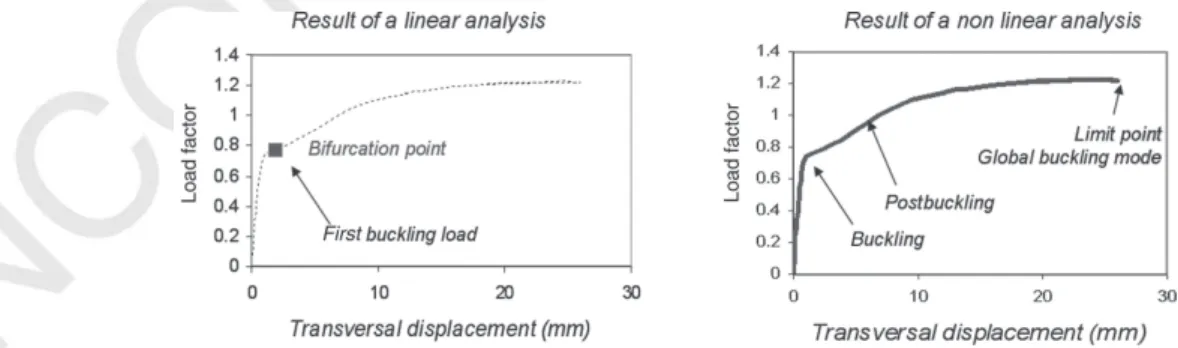
estimates of the stiffness of the structure and the ply resistance, with classical first ply failure criteria such as Tsai–Hill [8]. Buckling can also be studied enabling the bifurcation points, which are the intersections of different (stable or unstable) equilibrium paths [6], to be identified. Figure 5 presents the local and global buckling modes appearing in a curved composite structure made of six super-stiffeners (hat stiffeners) submitted to shear and compression. These structural responses can be computed at the component (local) level (Fig. 4) or at the whole structural level (global level).
Geometric Nonlinearities. The reliability of a linear buckling analysis is questionable for structures capable of withstanding large displacements observed beyond a bifurcation point in the postbuckling range or those assum-ing a limit point in the equilibrium path. To simulate
such behaviors more realistically, a nonlinear analysis is needed to identify the collapse (limit) load of the structure. Figure 6 illustrates the equilibrium path of the composite structure shown in Fig. 5 when it sustains buckling and postbuckling, up to the final collapse. The inclusion of geo-metrical nonlinearities in the analysis enables the design of lighter structures by allowing them to operate in the postbuckling state [9].
Material Nonlinearities and Damage Tolerance. Delami-nation and fiber and matrix breaks are typical composite failure modes, which must be taken into account in the design of structural composites [1,10,11]. In most cases, simplified criteria are applied in the preliminary design phase to obtain a damage tolerant structure. Examples of such criteria can be found in Refs 8 and 12.
For more information on the FEM, and especially the discretized equations of the physical phenomena described above, refer to Ref. 2.
Integrated Analysis of Large Composite Structures
The design of large stiffened composite structures used in aeronautics is carried out by the combination of a global analysis on the whole structural model and local
Figure 7. Global/local analysis of a complex composite structure.
3. Update the global model with new values of the local
parameters
Ny
Px Nx Nxy
computations on the super-stiffeners. The forces acting on each super-stiffener are obtained from the global FEM analysis. They form input for the local analyses, which are conducted as described previously. At this local level, the values of the parameters (e.g., ply thickness, fraction of 90◦ plies) can be modified in order to provide a safe design. Since local modifications alter the global structural Q2
behavior, the global model is updated and a new global analysis is carried out, in order to re-evaluate the local forces modified by the new values of the local parameters (Fig. 7).
THE STRUCTURAL COMPOSITE OPTIMAL DESIGN Introduction
The use of optimization algorithms is essential in order to assign optimal values to the numerous parameters defining the mechanical properties of structures made of fiber-reinforced composite materials. These parameters influencing the composite design, called the design vari-ables, can be the number of plies, their thickness and fiber orientation, the stacking sequence, and the shape and topology of the structure. The structural responses of com-posites, for example, the buckling load, the strain energy density, the ply strains, and failure indices, can typically present highly nonlinear and nonmonotonous behaviors with respect to the design variables. As a result, the opti-mization problem is extremely difficult to solve, since it is not convex and therefore characterized by several local optima and many infeasible solutions. Moreover, when the optimization of the stacking sequence is addressed, the problem is combinatorial and specific solution procedures are required. The optimal design of composite structures has been studied for more than 30 years, and although several interesting solutions have been proposed, a gen-eral solution procedure still has not been obtained. The key point of these optimization procedures relies on how the plies and laminates are parameterized. In this section, after a brief review on how a structural optimization prob-lem is formulated, the main innovative concepts developed over the past years for the structural composite optimal design are described and discussed.
The Mathematical Optimization Problem
The optimization problem is written in Equation (1). It includes one objective function g0(x) to be minimized and
m constraints gj(x). These functions depend on n design variables x = {xi=i = 1, . . . , n}, which are the parameters Q3 whose values are varied to find an optimal solution. At the optimum, each constraint must be lower than or equal to a given value gj. Side constraints are added to the problem, providing lower and upper limits on the design variable values, representing physical or manufacturing restrictions.
min
x g0(x) submitted to gj(x) ≤ gj, j = 1, . . . , m and xi≤xi≤xi, i = 1, . . . n. (1) The functions gjin the problem (1) are generally non-linear. They can be global and impact the whole structure, as is the case for the structural stiffness, the buck-ling loads, or the vibration frequencies. They can also be local, and so defined in each ply, examples of which are the Tsai–Wu and Tsai–Hill criteria. The solution of problem (1) is obtained iteratively. At each iteration, a structural analysis is carried out, the results of which feed the optimizer which provides new values for the design variables. Several optimization methods exist and can be used to solve the problem (1). Gradient-based meth-ods, such as the mathematical programming methods [13] and the sequential convex programming methods [14] use the first-order derivatives of the structural functions. Zero-order methods, such as the genetic algorithms [15] or the surrogate-based optimization methods [16], use only the function values. The latter requires a large number of structural analyses but can be used directly when the gradients are not available.
The Optimal Design of Structural Composites: Aspects and Considerations
The ultimate goal of composite design is to define zones of optimal stacking sequences in the structure (Fig. 1). This is clearly a complicated task, since this is a combinatorial problem including a very large number of parameters and restrictions. In aircraft applications, conventional laminates made of stacking sequences of 0◦, 45◦, 90◦, and −45◦fiber angles have been used. With
Figure 8. Draping of six plies, with continuity con-straints over the regions of different thickness.
Figure 9. Summary of the methods used for the optimal design of structural compos-ites.
the improvement of manufacturing capabilities and especially the developments of advanced fiber and tape placement machines, it is now possible to design struc-tures with curved fibers. Allowing fiber orientations that change continuously over the structure with respect to the local internal forces improves the design, as reported in Ref. 17. For conventional laminates, specific and compli-cated design rules related to mechanical or manufacturing requirements should be taken into account. Some of them impact the ply continuity of the draping, as illustrated in Fig. 8. Others stipulate that, for damage tolerance considerations, no more than four consecutive superposed plies should have the same orientation. Such constraints are clearly difficult to take into account in the formulation of the optimization problem.
Confronted with such difficulties, it is thus under-standable that a global and general solution for the optimal structural composite design is not yet available. An overview of the many approaches studied over the past 30 years is shown in Fig. 9 and reviewed in the following sections.
Parameterizations of Composites in View of Their Optimal Design
Depending on the choice of the design variables in (1), different optimization problems can be addressed. Vari-ous parameterization formulations have been proposed for composite structures, each of them with their own advan-tages and disadvanadvan-tages, as discussed in the following sections. In order to introduce the notations, the constitu-tive relations in a ply with unidirectional fiber orientation and the classical lamination theory are briefly reviewed.
Constitutive Relations for the Orthotropic Ply and the Laminate [8]. The constitutive relations of an orthotropic composite ply in its orthotropic axes are given in (2) for a plane stress state, where Exand Eyare the Young modulus
in the longitudinal and transverse directions, Gxyis the shear modulus, and νxyis the Poisson ratio:
σx σy σxy = mEx mνyxEx 0 mνxyEy mEy 0 0 0 Gxy εx εy γxy = Qxx Qxy 0 Qyx Qyy 0 0 0 Qss εx εy γxy m = 1 1 − νxyνyx . (2) The constitutive relations of an orthotropic composite ply having an orientation θ with respect to the structural (or laminate) axes is given in (3), where the three indices 1, 2, and 6 stand for the global longitudinal direction, the transversal direction, and the shear direction, respectively (Fig. 10). σ1 σ2 σ6 = Q11(θ ) Q12(θ ) Q16(θ ) Q12(θ ) Q22(θ ) Q26(θ ) Q16(θ ) Q26(θ ) Q66(θ ) ε1 ε2 ε6 σ = Q(θ )ε. (3) The stiffness coefficients Qij(θ ) in (3) are related to the orthotropic coefficients Qxx, Qyy, Qxy, and Qssin (2) by trigonometric functions either of the fourth power (e.g., sin4θ , cos4θ , sin2θ cos2θ , sin3θ cos θ , . . .) or depending on multiples of the angle θ (sin 2θ , sin 4θ , cos 2θ , and cos 4θ ). In this case, it can be shown that
Q(θ ) = γ0+ γ1cos 2θ + γ2cos 4θ + γ3sin 2θ + γ4sin 4θ , (4) where the 3 × 3 matrices γ are functions of the orthotropic coefficients Qxx, Qyy, Qxy, and Qss
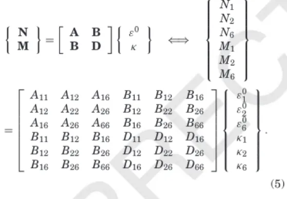
In the classical lamination theory, the constitutive rela-tions of the laminate are expressed in (5), where A, B, and D are the in-plane (membrane), coupling, and bend-ing stiffness matrices, N and M are the local forces and moments by unit length, and ε0 and κ are the in-plane
(laminate) Matrix
Figure 10. Laminate including four plies: structural axes (1,2,3) and material axes (x, y, z).
Figure 11. Definition of the plies location through the laminate’s thickness.
2 1 hk hk–1 h0 h1 h2 n 3 k 1 zk tk h
strain and curvatures, respectively. The stiffness matrices are obtained by considering the superposition of n plies with their own properties given by (3), using the notations of Fig. 11. ½ N M ¾ = · A B B D ¸ ½ ε0 κ ¾ ⇐⇒ N1 N2 N6 M1 M2 M6 = A11 A12 A16 B11 B12 B16 A12 A22 A26 B12 B22 B26 A16 A26 A66 B16 B26 B66 B11 B12 B16 D11 D12 D16 B12 B22 B26 D12 D22 D26 B16 B26 B66 D16 D26 D66 ε10 ε20 ε60 κ1 κ2 κ6 . (5) Direct Parameterization. When the thickness tkand the fiber orientation θk of each ply k are defined to describe the laminate, the coefficients of the stiffness matrices in (5) can be written as follows:
Aij= n X k=1 [Qij(θk)]tk Bij= n X k=1 [Qij(θk)]tkzk Dij= n X k=1 [Qij(θk)] Ã tkz2k+ t3 k 12 ! . (6)
From (6), it is seen that B is equal to zero for sym-metric laminates. In addition, the position of the plies in the stacking sequence has no influence on the mem-brane stiffness coefficients, but this does have a strong influence on the flexural behavior of the laminate. The parameters tk and θk can be the design variables of the
optimization problem (1). For a laminate, 2n design vari-ables are necessary, so in practice, the number of design variables can become very large. Moreover, it can be seen that the optimization problem expressed with such design variables is highly nonlinear and nonmonotonous and not convex. It is therefore difficult to find a solution, and only local optima can be identified. However, such design variables are meaningful for the user and have a direct physical interpretation. Applications using this approach can be found in Refs [18–20]. When discrete design vari-ables are used, for the thickness and orientation, specific optimization algorithms must be used [21].
The Black Metal Concept: Homogenized Laminate. In an homogenized laminate, the coefficients of the A, B, and D matrices are given by
Aij= n X k=1 [Qij(θk)]tk Bij=0 Dij= h2 12Aij, (7) where h is the total thickness of the laminate. The fibers proportions %0◦, %90◦, %45◦, and %−45◦that correspond to the conventional plies at 0◦, 90◦, 45◦, and −45◦are given by the following relations:
%j◦= n X k=1 tk¡θ = j◦¢/h, j = 0, 90, 45, −45 %0◦+%90◦+%45◦+%−45◦=1. (8)
These four proportions and the total thickness h of the laminate can be used to parameterize the composite. They describe the in-plane stiffness A and the flexural behavior D via Equation (7). As carbon fibers are used for advanced aircraft applications, and since the material is homogeneous, like metal, this parameterization is termed black metal [22]. Considering Equation (8) for orthotropic
laminates, three design variables, h, %0◦, and %90◦, are sufficient. The disadvantages of this parameterization are that approximations are made in the evaluation of the D matrix, the notion of stacking sequence is lost, and that the flexural behavior is approximated. An approximated bending stiffness matrix D can lead to inaccuracies in the simulation of buckling, but this approach can be used in a preliminary design phase.
Lamination Parameters. On the basis of relation (4), it is possible to express the laminate stiffness matrices A, B, and D as linear functions of specific parameters, termed the lamination parameters:
A = hγ0+ γ1ξ1A+ γ2ξ2A+ γ3ξ3A+ γ4ξ4A, B = γ1ξ1B+ γ2ξ2B+ γ3ξ3B+ γ4ξ4B, D =h 3 12γ0+ γ1ξ D 1 + γ2ξ2D+ γ3ξ3D+ γ4ξ4D, (9) where γ are material invariants [23] and the lamination parameters are defined as
ξ[1,2,3,4]A,B,D = h/2 Z
−h/2
z0,1,2£cos 2θ(z), cos 4θ(z), sin 2θ(z),
sin 4θ (z)¤ dz, (10)
where θ (z) is the transverse angle distribution and h is the total thickness of the laminate. Note that, each stiffness matrix depends on four lamination parameters, and there are 12 in total irrespective of the number of plies in the laminate. Simplifications are possible, such as when the laminate is symmetric, the four lamination parameters related to the coupling matrix B are equal to zero. Moreover, only two lamination parameters are needed to express the membrane (bending) stiffness A (D) if the laminate is balanced and orthotropic.
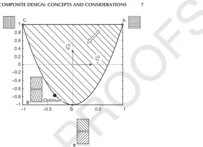
Using lamination parameters for the lay-up optimiza-tion significantly reduce the number of design variables in comparison with using ply orientations and thicknesses. Moreover, the feasible region for optimization in the design space of the lamination parameters is convex, so the opti-mum can be easily obtained with significant computational time savings. Figure 12 shows the region and the optimum solution for a bending problem of orthotropic laminates. Other optimum design solutions are shown in Table 1. However, determining the feasible region is not trivial, and even though the feasible regions were identified for most common applications [24–26], a general solution is still missing. –1 –0.5 0.5 1 –1 –0.8 –0.6 –0.4 –0.2 0 0.2 0.4 0.6 0.8 1 A B C ξD 2 ξD 1 Optimum
Figure 12. Feasible domain of the lamination parameters for the bending of an orthotropic laminate.
The lamination parameters are related to the stiffness (6), which is a global property of the laminate. This means that when lamination parameters are used, the informa-tion at the ply level is lost. Although first ply failure constraints can be defined within the design space of lam-ination parameters [27], once the optimal values of the lamination parameters are obtained, it is necessary to identify the number of plies and the corresponding fiber orientations. This is usually a discrete design problem that can be solved with a meta-heuristic procedure such as genetic algorithms [28] or branch and bound [29].
Ply Selection Based on Topology Optimization. This parameterization is presented for the case in which conventional laminates with plies oriented at 0◦, 45◦, 90◦, and −45◦must be distributed in a composite part divided in zones of constant stacking sequence (Fig. 13). The constitutive matrix Q of each ply is replaced by a linear combination of the constitutive matrix Qi of the four candidate plies (8). At the solution only one wimust have a value equal to one, while the others are equal to zero. The weighting coefficients widepend on design variables. The selection of correct weighting coefficients is the key point of the method and is discussed in Refs 30 and 31. The solution provides the best local orientations, as illustrated in Fig. 13, allowing the resulting pattern to
Table 1. Summary of Some Important Results Obtained with the Lamination Parameters
Structures Configuration Criteria Optimal Sequence
Plate Symmetric and orthotropic Stiffness, vibration, buckling [(±θ)n]S
Symmetric Buckling [θ]S
Membrane Symmetric Stiffness [(α/90 + α)n]S
General Stiffness [θ], [α/90 + α]
Figure 13. Distribution of conventional plies in the structure.
Figure 14. Illustration of a global parameterization of the ply.
be interpreted as a curved fiber distribution. However, the method can provide a design with rapidly varying fiber angles, which is difficult to interpret. Moreover, the optimization problem is not convex and the global optimum may not be obtained.
Q = w1Q(0◦) + w2Q(45◦) + w3Q(90◦) + w4Q(−45◦). (11) Global Parameterization. To avoid the disadvantage of the previous parameterization, the curved fibers can be defined over the whole structure, rather than being deter-mined in small regions, with a mathematical description
including few geometric design variables, as illustrated in Fig. 14. A reference fiber is first generated, which is then translated to represent the whole ply [17,32]. The advantage of this formulation is to decrease the number of design variables and to provide a design better suited to the capabilities of the automated tape and fiber placement machines. However, the optimization problem remains nonconvex [33].
Use of Discrete Optimization Methods. According to its combinatorial nature, the solution of the stacking sequence problem can be addressed with zero-order discrete opti-mization methods also termed meta-heuristic strategies. Various meta-heuristics are available, the most popular being the genetic algorithms [15]. With this approach, a population of candidate solutions is created and parame-terized in terms of chromosome and genes. The algorithm uses the process of natural selection by mimicking the con-cept of survival of the fittest. The population evolves over generations (iterations), and finally, the process identifies the best solution. Such an approach has been used in Refs 34 and 35. The size of the population depends on the number of design variables in the problem, which has a significant effect on the computational time. Other meta-heuristics proposed for laminated composite discrete optimization are branch and bound [29], simulated anneal-ing [36], tabu search [37], and particle swarm optimization Q4 [38]. Note that in order to be computationally effective,
Figure 15. Illustration of the two-step optimal design approaches.
such heuristic methods require implementation of rules of thumb and tuning of various parameters based on the in-depth knowledge of the specific problem at hand. Usu-ally such tuning cannot be generalized if the problem conditions change.
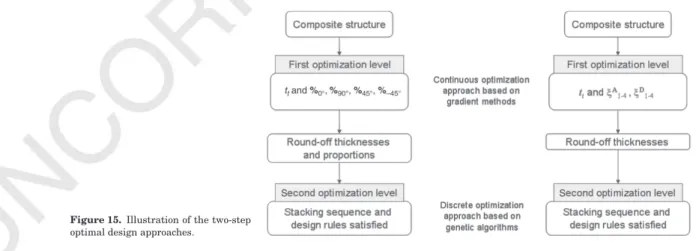
Two-Step Optimization. Confronted with the difficulty Q5
in determining the number of plies, their shape, and the local stacking sequences simultaneously, while satisfying design rules and ply continuity constraints over the zones of complex structures (Figs 1,7, and 8), some researchers have proposed a two-step solution to solve the optimal design problem (Fig. 15). The first step involves determin-ing the optimal thickness and the proportions of conven-tional plies in each zone based on the global/local scheme shown in Fig. 7. This result is obtained using either a black metal parameterization [22] or the lamination parameters. The second step addresses the stacking sequence problem, using a strategy based on genetic algorithms and global sublaminates to identify the plies distribution satisfying the manufacturing design rules [39,40].
CONCLUSIONS
The structural composite design is an extremely com-plicated task conducted nowadays with computers and numerical tools. It involves several disciplines, including CAD, CAE, and CAM, in an iterative process where opti-mization plays a very important role. According to the large number of parameters needed to design a composite structure, optimization methods are essential to identify the optimal stacking sequences, which is the ultimate goal of the design process. Several approaches have been pro-posed over the past years, but a global solution is not yet available. The ultimate solution procedure should address the problem at the CAD–CAE–CAM levels simultane-ously, in order to provide light and safe designs that are ready to be used in manufacture.
REFERENCES
1. Baker A, Dutton S, Kelly D. Composite materials for aircraft structures. AIAA Education Series. Reston; 2004. Q6
2. Zienkiewicz OC. The finite element method. McGraw-Hill; 1977.
3. VISTAGY web information: www.vistagy.com. Q7
4. CGTECH web information: www.cgtech.com.
5. O’Connor J. Software to enable composite and assem-bly development processes for modern airframes. 2nd International Carbon Composites Conference; October 27; Arcachon, France. 2009.
6. Falzon B, Hitchings D. An introduction to modeling buck-ling and collapse. NAFEMS Ltd; 2006.
7. Bisagni C, Vescovini R. J Aircr 2009;46(6):2041–2053. 8. Tsai SW. Strength & life of composites. Stanford
Aero-nautics & AstroAero-nautics - JEC Composites; 2008. 9. Bruyneel M, Colson B, Delsemme JP, et al. Int J Struct Q8
Stab Dy 2010.
10. Bruyneel M, Delsemme JP, Jetteur P, et al. Appl Compos Mater 2009;16:149–162.
11. Krueger R. Appl Mech Rev 2004;57:109–143.
12. Herencia JE, Weaver PM, Friswell MI. AIAA J 2009;45(10):2497–2509.
13. Bonnans JF, Gilbert JC, Lemar´echal C, et al. Numerical optimization: theoretical and practical aspects. Berlin: Springer; 2004.
14. Fleury C. Rozvany GIN editors. Volume I, Sequential con-vex programming for structural optimization problems. Optimization of Large Structural Systems. The Nether-lands: Kluwer Academic Publishers; 1993. pp 531–553. 15. Goldberg D. Genetic algorithms in search, optimization
and machine learning. Addison-Wesley Reading; 1989. 16. Liu B, Haftka RT, Akgun MA. Struct Optimization
2000;20:87–96.
17. Hyer MW, Charette RF. AIAA J 1991;29:1011–1015. 18. Mota Soares CM, Mota Soares CA. Compos Struct
1995;32:69–79.
19. Bruyneel M. Compos Sci Technol 2006;66:1303–1314. 20. Pedersen P. Struct Optimization 1991;3:69–78. 21. Beckers M. A dual method for structural optimization
involving discrete variables. 3rd World Congress of Struc-tural and Multidisciplinary Optimization; 17–21 May; Amherst (NY). Amherst (NY): 1999.
22. Krog L, Bruyneel M, Remouchamps A, et al. COMBOX: a distributed computing process for optimum pre-sizing of composite aircraft box structures. 10th SAMTECH Users Conference; 1314 March; Li`ege, Belgium. Li`ege, Belgium: 2007.
23. Tsai SW, Pagano NJ. Invariant properties of compos-ite materials. Composcompos-ite Materials Workshop. Westport (CT): Technomic Publishing; 1968. pp 233–253. 24. Fukunaga H, Sekine H. AIAA J 1992;30:2791–2793. 25. Diaconu CG, Sekine H. AIAA J 2004;42:2153–2163. 26. Bloomfield MW, Diaconu CG, Weaver PM. Proc Roy Soc
2009;465(2104):1123–1143.
27. IJsselmuiden ST, Abdalla MM, Gurdal Z. Imple-mentation of Strength Based Failure Criteria in the Lamination Parameter Design Space 48th AIAA/ASME/ASCE/AHS/ASC Struct. Struct Dynam, and Mat Conf; 23–26 April 2007; Honolulu, Hawaii. Honolulu, Q9 Hawaii.
28. Herencia JE, Weaver PM, Friswell MI. Local optimi-sation of anisotropic composite panels with T shape stiffeners. In Forty-eighth AIAA/ASME/ASCE/AHS/ASC Struct., Struct Dynam, and Mat Conf; 23–26 April; Hon-olulu, Hawaii. HonHon-olulu, Hawaii: 2007.
29. Matsuzaki R, Todoroki A Compos Struct 2007;4:537–550. 30. Stegmann J, Lund E. Int J Numer Meth Eng
2005;62:2009–2027..
31. Bruyneel M. Struct Multidiscip O. 2010.
32. Tatting BF, Gurdal Z. Automated finite element analy-sis of elastically-tailored plates. NASA/CR-2003-212679, Q10 2003.
33. Dems K, Wisniewski J. Optimal fibers arrangements in composite materials. 8th World Congress on Structural and Multidisciplinary Optimization; 1–5 June; Lisbon, Portugal. Lisbon, Portugal: 2009.
34. Le Riche R, Haftka RT. AIAA J 1993;31(5):951–956. 35. Kin CC, Lee YJ. Compos Struct 2004;63(3):339–345. 36. Erdal O, Sonmez F. Compos Struct 2005;71(1):45–52. 37. Pai N, Kaw A, Weng M. Compos Part B-Eng
materials. Proceedings of the International Symposium on Computational Structural Engineering; 22–24 June; Shangai, China. Shangai, China: 2009.
![Figure 2. Illustration of the CAD and CAM capabilities for the design of a fuselage [3,4].](https://thumb-eu.123doks.com/thumbv2/123doknet/6048415.151751/2.892.153.887.186.818/figure-illustration-cad-cam-capabilities-design-fuselage.webp)