Solvability and numerical simulation of BSDEs related to BSPDEs with applications to utility maximization

(1)

Solvability and numerical simulation of BSDEs related to

BSPDEs with applications to utility maximization

Peter Imkeller

Institut f¨ur Mathematik Humboldt-Universit¨at zu Berlin

Unter den Linden 6 10099 Berlin [email protected]

Anthony R´eveillac

Jianing Zhang

April 6, 2010

Abstract

In this paper we study BSDEs arising from a special class of backward stochastic partial differential equations (BSPDEs) that is intimately related to utility maximization problems with respect to arbitrary utility functions. After providing existence and uniqueness we dis-cuss the numerical realizability. Then we study utility maximization problems on incomplete financial markets whose dynamics are governed by continuous semimartingales. Adapting standard methods that solve the utility maximization problem using BSDEs, we give so-lutions for the portfolio optimization problem which involve the delivery of a liability at maturity. We illustrate our study by numerical simulations for selected examples. As a byproduct we prove existence of a solution to a very particular quadratic growth BSDE with unbounded terminal condition. This complements results on this topic obtained in [6, 7, 8]. 2010 AMS subject classifications: Primary: 60H30, 93E20; Secondary: 60H35, 65C05. JEL subject classifications: Primary: C61; Secondary: C63.

Key words and phrases: BSDE, BSPDE, logarithmic transformation, distortion transforma-tion, quadratic growth, utility optimizatransforma-tion, stochastic optimal control, numerical scheme.

Introduction

Portfolio optimization is a long-standing subject of mathematical finance which is closely related to fundamental issues like the pricing and hedging of contingent claims and to stochastic control theory. In this paper we study an investor whose trading window is given by a finite time interval [0, T ] and who can trade risky assets and one riskless bond. Upon choosing a risk preference, the investor aims at optimizing her expected utility from terminal wealth which is subject to the delivery of a liability. This objective can be formulated as the stochastic control problem

sup

π E[U (x +

Z _T

0

πudSu− F )] (1)

where U : R → R is a deterministic utility function, S a stochastic process modeling asset prices on a financial market and π the strategies that the investor is allowed to follow. In incomplete markets, a deep and powerful approach to solving (1) is provided by duality theory and has been

(2)

studied extensively (see for example [3] for a review; we also refer to [9, 26, 20, 4] for a non exhaustive list of references). This approach translates the absence of completeness onto the set of equivalent martingale measures and derives a dual problem which consists of characterizing an optimal portfolio by an optimal martingale measure and then to re-interpret the solution of the primal problem via convex duality theory. Its strength is that it ensures the existence or/and uniqueness of an optimal strategy π∗ _{for the problem (1) for very general utility functions U .}

However the solution of the dual problem is in general not constructive and finding explicit form solutions for the dual problem is a sophisticated task. Due to this lack of tractable constructive solutions, to the best of our knowledge, no numerical approximations of duality theory solutions are available yet. Another method consists of directly relating the stochastic control problem (1) to a Backward Stochastic Differential Equation (BSDE), which is an equation of the form

Yt= ξ + Z _T t f (s, Ys, Zs)ds − Z _T t ZsdWs. (2)

This approach directly attacks the primal problem and constructively describes the optimal solution in terms of the BSDE (2). In [14], the authors construct in a Brownian setting su-permartingales Rπ _{depending on the investor’s strategy π such that at maturity, R}π

T coincides

with the terminal wealth of the investor. They replace the martingale measure characteriza-tion of incompleteness by an martingale optimality principle, which roughly speaking solves (1) by finding some π∗ _{such that R}π∗

is a martingale which evidently yields the optimal expected utility at time zero. Key to constructing the supermartingales Rπ _{which eventually satisfy the}

martingale optimality principle is implementing the BSDE (2) into the construction. This op-timality paradigm has been extended in the works [24] [22] for general utility functions where the authors characterize the optimal solution of (1) by a nonlinear Backward Stochastic Partial Differential Equation (BSPDE). Yet, existence and uniqueness of such nonlinear BSPDEs are not shown and to the best of our knowledge, no existence (and uniqueness) statements seem to exist. However [22] shows that for classical utility functions (exponential, power and logarith-mic) these nonlinear BSPDEs reduce to an a priori new quadratic growth BSDE (of the form (24)) with a generator exhibiting a fraction that contains a denominator term in Y . This type of quadratic BSDEs is clearly beyond the limits of the usual requirements (e.g [19]) that ensure existence or/and uniqueness. In the recent paper [25] the optimization problem with respect to the power utility function with consumption formulated by a BSDE as in [22] has been solved. In this paper we consider the BSDEs obtained from the BSPDEs in [22] as just described. We propose a two-step reduction algorithm to transform them into coordinates in which ex-istence and uniqueness results are available, and ultimately in which they are accessible for efficient numerical approximation schemes. In a first step, we systematically employ the method of logarithmic change of variables, to establish existence and uniqueness results. This change of variables was previously used in [15] to solve a coupled FBSDE in a very special case. In this way, we are able to reduce these BSDEs by a one-to-one map to standard quadratic BSDEs, for which all tools and results for the classical form of quadratic BSDEs are available. In a second step, within a predictable representation framework, we provide another one-to-one map which relates this new quadratic growth BSDEs to linear ones. This technique has been employed in [29] under the term distortion transformation on the level of PDEs to linearize an HJB equation.

The completion of this two-step algorithm sets the stage for a numerical approach of the BS-DEs from [22], and henceforth also for their corresponding portfolio optimization problems. Quadratic BSDEs are characterized by a driver f (t, y, z) of quadratic growth in z. Existence

(3)

and uniqueness results for these quadratic growth BSDE have been established in [19]. How-ever the numerical treatment of such quadratic BSDEs has only been realized recently in [10], [16]. Another method for numerically solving quadratic BSDEs can be found in [17]. It em-ploys a method which similarly transforms quadratic BSDEs to BSDEs with Lipschitz continuous drivers, and as such amenable to efficient (especially in higher dimensions) Monte-Carlo schemes as investigated in [2], [5], [13]. In our opinion, the features of easy realizability and computa-tional performance of numerical methods for BSDEs provide an attractive complement to the theoretical results obtained in the first part of the paper.

The paper is organized as follows. In Section 1 we introduce the notation and specify the probabilistic setting we are working with. We then present an existence and uniqueness result for the type of quadratic BSDEs involving the denominator with the value process. We further discuss their links to standard linear and quadratic BSDEs, and finish with a discussion about numerical methods. In Section 2 we apply the results to utility maximization problems. In particular, we consider different versions of portfolio optimization problems with respect to the delivery of a liability at maturity. If the liability possesses a representation with respect to the underlying martingale, the optimization problem with the liability is tackled as an optimization problem without liability involving strategies shifted by the representation density. We realize that the BSDE results obtained in the previous section yield an alternative approach to portfolio optimization with respect to the power and the exponential utility. An interesting by-product of our analysis can be found in Section 2.1.2: an existence and uniqueness result for quadratic BSDEs with general unbounded terminal conditions. Though owing to its particular structure, we feel that this result complements the analysis done in [6, 7, 8]. We conclude in Section 3 with the presentation of numerical simulations for selected utility maximization problems.

1 BSPDEs and their reduction to BSDEs

The objective of this Section is to provide an analysis of the special class of BSPDEs derived in [22] and [24]. We will focus on the link to BSDE discussed in [22] which, in the context of utility optimization problems, provides solutions to BSPDE once the utility function exhibits certain features. To this end, we briefly depict the probabilistic setup we will be working with.

1.1 Preliminaries and notations

Let T ∈ R+ = [0, ∞) denote the terminal time. We work on a probability space (Ω, F, P)

endowed with a continuous and complete filtration (Ft)0≤t≤T, which governs an Rd×1-valued

continuous local martingale M = (M1_{, . . . , M}d₎tr_{. By tr we denote the transpose of real valued}

vectors. We call a filtration (Ft) continuous if every R-valued square integrable, (Ft)-adapted

martingale N is continuous and yields the representation Nt= N0+

Z _t

0

Z_strdMs+ Lt, 0 ≤ t ≤ T, (3)

where Z is a predictable process with values in Rd×1 _{and L a real valued square integrable}

martingale strongly orthogonal to M , i.e. hMk_{, Li = 0 for every k ∈ {1, . . . , d}. Given any}

probability measure Q on (Ω, F), we denote by EQ the expectation with respect to Q and omit the superscript if Q is equal to the original measure P. The Kunita-Watanabe inequality (see e.g. Theorem 25 in [27]) implies that each covariation hMk_{, M}l_{i, k, l ∈ {1, . . . , d}, is absolutely}

(4)

continuous with respect to the process C = Pd_k=1hMk_{, M}k_{i. Hence there exists an increasing}

and bounded continuous process K, e.g. given by K = arctan(C), such that the quadratic variation hM, M i satisfies the structural representation

dhM, M i = σσtrdK, (4)

where σ is a predictable process with values in Rd×d_{such that σ}

tσtrt is almost surely invertible for

every t ∈ [0, T ]. We denote the Euclidean norm of vectors x ∈ Rd×1 _{by |x| = (x}tr_x)12. Moreover

for m ∈ N we denote by

• H2_(Rm_{, Q, σ) the space of all predictable processes Z taking values in R}m×1 _{such that}

EQhRT

0 |σsZs|2dKs

i < ∞;

• S∞_(Rm_{) the space of all bounded continuous R}m×1_{-valued processes Y = (Y}

t)0≤t≤T ;

• M2([0, T ], Q) the space of all real valued and square integrable martingales under the measure Q, adapted to (Ft)0≤t≤T, starting in zero.

If there is no ambiguity about m or Q, we omit referencing to Rm_{, Q and σ and simply write}

H2_{, S}∞ _{and M}2_.

1.2 A backward stochastic partial differential equation related to utility max-imization problems

In the realm of utility maximization problems, it is well known that for the standard utility functions of the logarithmic, exponential and power type, linear and quadratic BSDEs provide a unique solution for the optimization problem (1). A prominent approach of deriving from (1) a BSDE of type (2) is assuming certain regularity that permits Itˆo’s formula to be applied and taking advantage of the explicit from of the standard utility functions. For rather general deter-ministic utility functions U : R+ → R (i.e. U is continuously differentiable, strictly increasing

and strictly concave) satisfying the Inada conditions U0(0) = lim x→U 0_{(x) = ∞,} U0(∞) = lim x→∞U 0_{(x) = 0,}

the situation becomes more involved and the classical version of Itô’s formula appears deficient because one cannot take advantage of the specific structure of the standard utility functions anymore. It turns out that the right tool to approach (1) is a version of Itô’s formula that is generally known in the literature under the name Itô-Ventzell’s formula. Making use of this, it has been shown in [22] and [24] that solving the optimization problem (1) with some general utility function U leads to the particular equation

V (t, x) = U (x) −1 2 Z _T t (ϕ_x(s, x) + λ_sV_x(s, x))tr Vxx(s, x) dhM, M i_s(ϕ_x(s, x) + λ_sV_x(s, x)) − Z _T t ϕ(s, x)trdM_s− Z _T t dL(s, x), (5)

where λ is a given Rd×1-dimensional predictable process and L(·, x) is a continuous one-dimensional martingale strongly orthogonal to M for all x. Since this equation is characterized by its termi-nal condition V (T, x) = U (x) and involves the partial derivatives ϕ_x, V_x and V_xx, it is called a

(5)

backward stochastic partial differential equation (BSPDE). If one has a solution (V, ϕ) of (5), one can characterize the optimal trading strategy and the optimal wealth process in terms of the BSPDE (we shall elaborate on this in more details in Section 2). We stress here that existence (and uniqueness) of solutions to equation (5) have neither been shown in [22] nor in [24] for the case of a general utility function U ; as the authors of these two works emphasize, the BSPDE (5) yields a verification tool, but solving it directly remains a challenging task.

We shall get across the message that we here are also not solving the BSPDE (5). We will rather provide a discussion of an ordinary version of (5) which on the one hand does not belong to the standard class of Lipschitz or quadratic growth BSDEs (but rather a mixture of both) and which on the other hand provides an alternative BSDE interpretation of solutions to utility maximization with respect to the power and the exponential function. More precisely, we investigate the BSDE

Vt= ξ + α Z _T t (ϕs+ λsVs)tr Vs dhM, M is(ϕs+ λsVs) − Z _T t ϕtr_sdMs− (LT − Lt), (6)

for which we assume that ξ ∈ L∞_{(R) is an F}

T-measurable random variable that is bounded

away from zero, i.e. there exists a constant c > 0 such that ξ ≥ c > 0 holds P-almost surely. We say that (V, ϕ, L) is a solution of the BSDE (6) if

(V, ϕ, L) ∈ S∞(R) × H2¡Rd×1, P, σ¢× M2([0, T ]) such that Vt> 0 for all t ∈ [0, T ].

The positivity condition on V stems from the fact that V will play the role of the value function. In the following we denote the solution spaces without their dimensions and parameters. In section 4 of [22], particular cases in which this BSDE admits a solution are considered, with methods of proof related to particular choices of ξ and the constant α. Yet we shall provide existence and uniqueness results for (6) using a different method. The key to showing existence and uniqueness of (6) is to find a suitable transformation relating (6) to the quadratic BSDE

Y_t= B + Z _T t f (s, Z_s)dK_s− Z _T t Z_strdM_s− (N_T − N_t) +1 2 Z _T t dhN, N i_s, (7) f (t, z) = ³ α + 1 2 ´ |ztrσt|2+ α ¡ ztrσtσttrλt+ λtrtσtσttrz ¢ + α|σtr_tλt|2, t ∈ [0, T ], z ∈ Rd, (8)

where B is a real valued bounded FT-measurable random variable, α a real number and λ an

Rn_{-valued predictable process. For this purpose we will use a logarithmic coordinate change}

which disentangles the denominator term of the driver of (6) and transforms it into the driver of a quadratic BSDE of the form (7). This type of transformation is employed in [15] in a Brownian setting to prove the existence and uniqueness of a fully coupled FBSDE with a quadratic growth backward equation by solving an equivalent linear FBSDE. We proceed similarly in our setup of a general continuous stochastic basis. Note that existence and uniqueness of the BSDE (7) have been studied in [23] and more recently some representations of the solution have been found in [18]. The next Lemma summarizes the conditions that guarantee existence and uniqueness of (7).

Lemma 1.1. Let B be an FT-measurable random variable which is bounded. Assume that there

exists a constant C > 0 such that we have P-almost surely R₀T |σtr

sλs|2dKs ≤ C. Then there

(6)

Proof. The hypothesis thatR₀T |σtr

sλs|2dKs ≤ C implies that the process |σtrλ| is almost surely

bounded. Hence the driver of equation (7) satisfies almost surely

|f (t, z)| ≤ |α + 1 2| |σ tr tz|2+ 2|α σttrλt| |σttrz| + |α| |σtrtλt|2 ≤ γ¡|α| |σtr_tλt|2+ |σtrtz|2 ¢ , t ∈ [0, T ], z ∈ Rd,

where γ is some non-negative real constant. Then Theorems 2.5 and 2.6 from [23] yield a unique triplet (Y, Z, N ) ∈ S∞_{× H}2_{× M}2_{([0, T ]) which solves BSDE (7).}

The following Lemma shows that depending on the sign of the constant α, the process V either becomes a sub- or a supermartingale. In the case of a supermartingale, V is even bounded away from zero.

Lemma 1.2. Let (V, ϕ, L) ∈ S∞_{× H}2_{× M}2 _{be a solution of}

Vt= ξ + α Z _T t (ϕs+ λsVs)tr Vs dhM, M is(ϕs+ λsVs) − Z _T t ϕtr_sdMs− (LT − Lt), t ∈ [0, T ],

where the terminal condition ξ is a non-negative and bounded FT-measurable random variable

such that there exists a constant c > 0 for which ξ ≥ c holds P-almost surely. Then for α > 0 we have that V is a supermartingale which possesses a lower bound c > 0. For α < 0 we have that V is submartingale.

Proof. Let α > 0. By definition of a solution (V, ϕ, L) of the BSDE, we have that Vt > 0 for

every t ∈ [0, T ] and it follows that for 0 ≤ s ≤ t ≤ T Vs = E h ξ + α Z _T s (ϕu+ λuVu)tr Vu dhM, M iu(ϕu+ λuVu) ¯ ¯Fs i ≥ E h ξ + α Z _T t (ϕu+ λuVu)tr Vu dhM, M iu(ϕu+ λuVu) ¯ ¯Fs i = E h Vt ¯ ¯Fs i .

Hence V is a supermartingale. This implies Vt≥ E h VT ¯ ¯Ft i = E h ξ¯¯Ft i ≥ E h c¯¯Ft i = c > 0

for every t ∈ [0, T ], i.e. V is even bounded away from zero. If α < 0, the same arguments show that V is a submartingale.

Next we prove the existence and uniqueness of solutions to (6). Proposition 1.3. Let ξ ∈ L∞ _{be a positive F}

T-measurable random variable which is bounded

away from zero. Let λ be a predictable process such that almost surely Z _T

0

|σ_strλs|2dKs≤ C

for some real constant C > 0 and let α be a nonzero real constant. Then the BSDE Vt= ξ + α Z _T t (ϕs+ λsVs)tr Vs dhM, M is(ϕs+ λsVs) − Z _T t ϕtr_sdMs− (LT − Lt), t ∈ [0, T ],

(7)

Proof. By the assumptions on the terminal variable ξ, the random variable B := log(ξ) is well-defined and also belongs to L∞_{(R). According to Lemma 1.1, there exists a unique triplet}

(Y, Z, N ) ∈ S∞_{× H}2_{× M}2 _{which satisfies BSDE (7) with the terminal condition B = log(ξ).}

Let us set P_t:= eYt_, ₍₉₎ Q_t:= eYt_Z t= PtZt, (10) R_t:= Z _t 0 eYs_dN s= Z _t 0 P_sdN_s, t ∈ [0, T ], (11) which by the existence of (Y, Z, N ) are well-defined. Note that since Y is bounded, the range of the process P lies in a compact subset of the real line that is bounded away from zero. This implies that Q ∈ H2 and hence R becomes a square-integrable martingale which is, due to the orthogonality of N to M , also orthogonal to M . An application of Itˆo’s formula from t to T in conjunction with (4) and (7) yields

Pt= ξ + α Z _T t µ |σ_strQs|2 Ps + Qtr_sσsσtrsλsPs Ps + PsλtrsσsσtrsQs Ps + |σ tr sλs|2Ps ¶ dKs − Z _T t Qtr_sdMs− (RT − Rt) = ξ + α Z _T t (Q_s+ λ_sP_s)tr Ps dhM, M i_s(Q_s+ λ_sP_s) − Z _T t Qtr_sdM_s− (R_T − R_t).

But this is exactly BSDE (6), hence setting (V, ϕ, L) = (P, Q, R) we have found a solution in S∞_{× H}2_{× M}2_.

In order to prove uniqueness, assume that (V1_{, ϕ}1_{, L}1_{) and (V}2_{, ϕ}2_{, L}2_{) are two solutions of (6).}

We apply the logarithmic change which in a first step amounts to defining a triplet (Yi, Zi, Ni) ∈ S∞_{× H}2_{× M}2 _via Y_ti = log(V_ti), Z_ti = ϕ i t Yi t , N_ti= Z _t 0 1 Vi s dLi_s, t ∈ [0, T ]. Note that by the definition of solutions (Vi_{, ϕ}i_{, L}i_{), i = 1, 2, we have V}i

t > 0 for every t ∈ [0, T ],

hence Yi _{is well defined. In a next step we apply Itˆo’s formula to Y}i _{and get the quadratic}

BSDE Y_ti= B + Z _T t α(Z_si+ λs)trdhM, M is ¡ Z_si+ λs) +1₂ Z _T t |Z_si|2dhM, M is − Z _T t (Z_si)trdM_s− (N_Ti − N_ti) +1 2 ¡ hNi, Nii_T − hNi, Nii_t¢ = B + Z _T t n¡ α + 1 2 ¢ |σ_strZ_si|2+ α¡(Z_si)trσsσtrsλs+ λtrsσsσtrsZsi ¢ + α|σ_strλs|2 o dKs − Z _T t (Z_si)trdMs− (NTi − Nti) + 1 2 ¡ hNi, NiiT − hNi, Niit ¢ , t ∈ [0, T ]. (12) For BSDEs of this type, comparison principles are available, see e.g. Theorem 2.7 in [23]. Taking into consideration that we have Y1

T = YT2= B, it follows by comparison that Yt1 = Yt2 and hence

also V1

(8)

E h Z T 0 ¯ ¯σtr sϕ1s− σtrsϕ2s ¯ ¯2 dKs i = E h Z T 0 |Y_s1|2 ¯¯σtr_sZ_s1− σ_strZ_s2¯¯2dKs i ≤ kY1k2_∞E h Z T 0 ¯ ¯σtr sZs1− σstrZs2 ¯ ¯2_dK s i | {z } =0 = 0,

where the uniqueness of the control process Z of BSDE (12) is used. Due to the uniqueness of N and V , it follows easily that we also have L1_{= L}2_.

Remark 1.4. In order to find solutions to (6), it is imperative to find a good transformation reducing it to some BSDE which we can handle. The core idea of the method of proof of Proposition 1.3 is comprised in the following observation: if we assume that the value process V is continuous, then for the continuity to be preserved by the driver of (6) the process V must stay either in the positive or the negative half of the real line, because otherwise V in the denominator of the driver will spoil continuity. Since we deal with utility values, it is reasonable to assume V to be positive. Then it becomes reasonable to perform the logarithmic change to V , that is, we set Y = log(V ) which is then well-defined. An application of Itˆo’s formula yields

dYt= ϕ tr t VtdMt+ 1 VsdLt− 1 2V2 t dhLit− α(ϕt+ λtVt) tr Vt dhM, M it (ϕt+ λtVt) Vt = ϕtrt Vt dMt+ 1 Vt dLt− 1 2V2 t dhLit− α µ ϕt Vt + λt ¶_tr dhM, M it µ ϕt Vt + λt ¶ , t ∈ [0, T ]. Introducing Zt= ϕt/Vt and dRt= dLt/Vt, the above equation can be written as

dY_t= Z_ttrdM_t+ dR_t−1

2dhRit− α (Zt+ λt)

tr_{dhM, M i}

t(Zt+ λt)

which is a BSDE with a driver of quadratic growth. These BSDE have been thoroughly inves-tigated in [21], [19] and more recently in [28]. The logarithmic transformation thus reduces the BSDE (6) to a BSDE with a quadratic generator which has been intensively studied and can be handled more easily.

1.3 A link to linear BSDEs

In the previous Section, we reduced the - from the perspective of BSDE theory - ”unusual” BSDE (6) to a more tractable quadratic growth BSDE (i.e. (7)) using a logarithmic transformation. We can go one step further in the same direction. If M possesses the martingale representation property, we can apply an exponential transformation to the BSDE (7) which then reduces to a linear BSDE. The latter are known to allow explicit solutions, see e.g. Proposition 2.2 of [12]. The exponential change aforementioned has been originally used in [19] and [23] to transform quadratic BSDEs into BSDEs that can be approximated by BSDEs with Lipschitz continuous drivers. In [17], this exponential coordinate change technique is used in a Brownian motion setting to transform quadratic BSDEs of the type appearing in Remark 1.4 into BSDEs with Lipschitz continuous drivers. In this form they become amenable to numerical approximation. The composition of the two transformations then leads to the power transformation detailed

(9)

below. We first consider martingales M which have the predictable representation property, i.e. every one-dimensional square integrable continuous martingale N yields the representation

N_t= N₀+ Z _t

0

Z_strdM_s, t ∈ [0, T ], (13) where Z is a uniquely determined square integrable predictable process. Then we reflect to the situation of (3) where the predictable representation property does not hold, and give a counterexample showing that in this setup the power transformation does not work in general. As it was pointed out to us, such a change of coordinate was used in [29] under the term distortion power change in the analytical context of PDEs. In [29] the author considers the HJB equations corresponding to an optimization problem, linearizes the dynamics via distortion and finds a (unique) viscosity solution to the HJB equation.

Assume that condition (13) is in force. Then BSDE (6) does not contain orthogonal martingales, i.e. L = 0. Now this BSDE admits a unique solution which is expressed as a solution of a linear BSDE raised to a certain power.

Proposition 1.5. Let ξ ∈ L∞ _{be a positive F}

T-measurable random variable that is bounded

away from zero. Let λ be a predictable process which satisfiesR₀T|σtr

sλs|2dKs≤ C almost surely

for some constant C > 0. Let α > 0. Then the BSDE Vt= ξ + α Z _T t (ϕs+ λsVs)tr Vs dhM, M is(ϕs+ λsVs) − Z _T t ϕtr_sdMs, 0 ≤ t ≤ T, (14)

admits a unique solution (V, ϕ) ∈ S∞_{× H}2 _{which can be written as}

Vt= Y 1 2c t , ϕt= Z_2ctY 1 2c−1 t , where c = α +1

2 and (Y, Z) ∈ S∞× H2 is the unique solution of the linear BSDE

Yt= ξ2c+ 2α Z _T t ¡ c|σ_strλs|2Ys+ Zstrσsσstrλs ¢ dKs− Z _T t Z_strdMs, t ∈ [0, T ]. (15)

Proof. According to Theorem 1.1 and Proposition 2.2 from [12], the linear BSDE (15) admits a unique solution (Y, Z) ∈ S∞_{× H}2 _{which is explicitly given by Y = H}−1_E£_ξ2c_H

T|F·

¤ and Z = H−1_{U + 2αY λ where H is the adjoint process}

The process U is predictable and square integrable as it appears via martingale representation in the formula

E£ξ2cH_T|F_t¤= E[ξ2cH_T] + Z _t

0

(10)

Since E£exp(R₀t|σtr

sλs|2dKs)

¤

≤ eC _{< ∞ for every t ∈ [0, T ], Novikov’s condition is satisfied so}

that E(2αR₀·λtr

sdMs)t is a uniformly integrable martingale giving rise to a probability measure

Q = E(2αR₀·λtr sdMs)T·P. By R_T 0 |σstrλs|2dKs≤ C it follows that e2α RT t |σstrλs|2dKs _{is almost surely}

bounded in t ∈ [0, T ]. Hence there exists a constant L > 0 such that Y_t= H_t−1E£ξ2cH_T|F_t¤= EQ£ξ2ce2αRtT|σstrλs|2dKs_|F

t

¤

≥ L > 0

holds Q-a.s. for every t ∈ [0, T ]. This means that Y is a non-negative process that is bounded away from zero Q-a.s. But since Q ∼ P, we also have that Y is P-a.s. bounded away from zero. Note that the second equality also shows that Y is a bounded process. Therefore the processes V = Y 2c1 and ϕ = Z

2cY

1

2c−1 are well defined and by Itˆo’s formula satisfy the BSDE

Vt= ξ + α Z _T t (ϕs+ λsVs)tr V_s dhM, M is(ϕs+ λsVs) − Z _T t ϕtr_sdMs, t ∈ [0, T ].

This shows the existence of a solution. For proving uniqueness, assume that (V1, ϕ1) and (V2_{, ϕ}2_{) are two solutions of equation (14). According to Lemma 1.2 both value processes are}

bounded away from zero, hence (Yi_{, Z}i_{) = ((V}i₎2c_{, 2c}ϕi

ViYi) for i ∈ {1, 2} are well defined, and

by the same arguments as above, (Yi_{, Z}i_{) satisfy the linear BSDE (15). By uniqueness of the}

solution (Y, Z) of the linear BSDE (15) (see e.g. [11]), Y1 = Y2 follows which in turn implies V1 _{= V}2_{. This gives rise to}

E h Z T 0 |σ_str(ϕ1_s− ϕ2_s)|2dKs ¯ ¯Ft i ≤ 1 4c2 ¡ kY k∞ ¢1 c−2 _E h Z T 0 |σ_str(Z_s1− Z_s2)|2dKs ¯ ¯Ft i = 0, showing that we have ϕ1 _{= ϕ}2 _{in H}2_.

Now let us go back to the setting of (6), i.e. a scenario in which the predictable representation property does not hold. If we try to extend the power transformation to (6) where L 6= 0, a formal application of Itˆo’s formula to Y = V2c _yields

Yt= ξ2c+ 2α Z _T t (cλsYs+ λtrsZs)dhM, M is− Z _T t Z_strdMs− Z _T t 2cYsdLs + Z _T t (c − 2c2)YsdhL, Lis, t ∈ [0, T ]. (16)

This BSDE is driven by a linear generator and solved by the process triple (Y, Z, L). Now this BSDE not only requires the orthogonal martingale to be of the specific form R 2cYsdLs, but

moreover contains a quadratic variation term in the orthogonal martingale which furthermore depends on the solution Y . We will see in the following example that BSDEs of this type do not admit solutions in general.

Example 1.6. Let (Ft) be generated by two independent one-dimensional Brownian motions

W1 _{and W}2_{. Set M = W}1 _{and ξ = W}2

T. Suppose that (Y, Z, L) is a solution of the zero

generator BSDE Y_t= W_T2− Z _T t Z_sdW_s1− Z _T t Y_sdL_s, t ∈ [0, T ].

(11)

Choosing t ∈ [0, T ] and conditioning with respect to Ftin the last line, we get on the one hand

Y_t= W2

t and on the other hand

Yt= Y0+ Z _t 0 ZsdWs1+ Z _t 0 YsdLs.

The covariation of the lefthand side withR₀·Z_sdW1

s is zero, and the covariation of the righthand

side isR₀·Z2

sds, implying that Z = 0 almost surely. Hence,

Yt= Y0+

Z _t

0

YsdLs

= Y0E(L)t,

Since Y0 = W02 = 0, it follows that Yt = 0 which contradicts Yt = Wt2. Hence this BSDE does

not have a solution.

1.4 Numerical tractability

The results of the previous sections essentially say that under certain conditions, the nonstandard BSDE (6) is equivalent to the standard quadratic BSDE (7) or, in a setting where we have the predictable representation property, even to the linear BSDE (15). Now if one works within a Brownian setting, the task of numerically approximating (6) becomes much more convenient because numerical schemes for BSDEs with Lipschitz drivers have been well studied in the literature, see e.g. [5], [13] and [2] for simulation based regression methods. We can use any of those schemes to solve the transformed BSDE (15) which by reverse transformation yields a numerical approximation of (14). One can even go further by approximating the quadratic BSDE (7) in a Brownian setting, since for this type of BSDEs, numerical approximation results are by now also available, see the recent works [16], [17].

In view of solving (possibly high-dimensional) utility maximization problems, BSDE schemes based on Monte-Carlo regression methods certainly are a practicable and computationally ef-ficient approach to numerical solutions. In dealing with multi-dimensional problems they are particularly favorable computationally in comparison with numerical methods for PDEs that solve the corresponding HJB equation. Moreover, computational implementability is the promi-nent difference between the BSDE and the convex duality approaches. Deriving solutions in the latter case that can be implemented or even deriving constructive solutions for the dual problem remain a challenging task in general (see e.g. [20, 4] and references therein). To the best of our knowledge, no numerical approximations relying on duality theory exist up to date. We give numerical examples of utility maximization problems in Section 3.

2 Applications to expected utility maximization problems

In this Section, we consider several utility maximization problems all of which yield a BSDE interpretation in terms of equation (6). The financial market is constituted by d risky assets S = (S1

t, · · · , Std)trt∈[0,T ] and one riskless bond which for the sake of simplicity is assumed to be

of zero interest rate. Let λ = (λ_t)_{t∈[0,T ]} be a predictable Rd×1_{-valued stochastic process which}

we specify at a later point. We exclude arbitrage opportunities within our market setup which corresponds to saying that the set of equivalent martingale measure Q ∼ P is not empty. As before let M be an Rd×1_{-valued continuous local martingale under P that satisfies condition}

(12)

(4). We assume that the market S evolves continuously in time, that is, S is a continuous Rd×1_{-valued stochastic process governed by}

dSt= dMt+ dhM, M itλt, t ∈ [0, T ]. (17)

On this market, private and institutional investors want to measure, control and manage risks as well as to speculate. We focus on an investor who is endowed with some initial capital x > 0. This investor buys and sells risky assets according to investment strategies which are Rd×1

-valued adapted stochastic processes π = (π_t)_{t∈[0,T ]} (πi _{is the share invested in the i-th stock S}i₎

satisfying EhR₀T |πu|2dhM, M iu

i

< ∞. By Xx,π _{we denote the wealth process of the investor}

associated to her initial capital and her chosen strategy (x, π), Xx,π = x +

Z _·

0

π_utrdSu. (18)

We call an investment strategy π admissible if in addition to square integrability, it satisfies X_tx,π ≥ 0 for every t ∈ [0, T ]. Our aim is to study an investor whose terminal wealth is subject to a FT-measurable liability F and who aims at maximizing her expected utility

V (0, x) := sup

π E

£

U¡X_Tx,π, F¢¤. (19) U denotes some utility function modeling the preferences of the investor and which is specified a few lines below. Due to the presence of the liability, the positivity constraint on the wealth, Xx,π ≥ 0, needs to be modified in each of the cases that we consider in the subsequent sections. The optimization problem (19) admits a solution if and only if the supremum in (19) is attained, that is if for every x ∈ R+ there exists an admissible strategy (π∗t(x))0≤t≤T such that

V (0, x) = E h U ³ X_Tx,π∗(x), F ´i .

In the following we consider two different notions of liabilities: additive liabilities that we in-vestigate in Section 2.1 and that correspond to U(x, y) := U (x − y) and multiplicative liabilities that we investigate in Section 2.2 which correspond to U(x, y) = U (xy). In both cases U denotes a deterministic utility function which we specify from case to case. More precisely, we consider utility maximization problems with respect to the power and the exponential utility and give their solutions in terms of BSDEs. We first consider optimizing a portfolio in presence of an additive liability. It turns out that for a special class of liabilities, some BSDE techniques de-veloped for utility maximization without liability (e.g. in [14], [22]) also work in this case. In a second step, we examine a multiplicative liability in the framework of the power utility function and provide BSDE characterizations for the optimal solutions, which have also been considered in [29] and [25].

2.1 Additive liability

Let U : dom(U ) → R be a utility function that is defined on a set dom(U ) ⊂ R and let U(x, y) = U (x − y). Then the optimization problem (19) can be rewritten as

V (0, x) := sup π E · U µ x + Z _T 0 π_utrdS_u− F ¶¸ , (20)

where F is a real valued and FT-measurable random variable that represents a liability the

(13)

relies on methods developed in [14] and [22], and due to this choice, we have to restrict the class of liabilities in the following way: F is a real valued F_T-measurable random variable which satisfies

• E[F2_{] < ∞ and}

• there exist a constant c and an adapted square integrable stochastic process (η_t)_{t∈[0,T ]} in Rd×1 _{such that}

F = c + Z _T

0

η_utrdSu. (21)

If this represents the class of all contingent claims, then condition (21) means that every claim F is replicated by the process η, implying that we are in the setting of a complete market. Since U is a priori defined on dom(U ), we define the set of optimal strategies Πηx by

Πη_x := ½ π : Ω × [0, T ] → Rd: E ·Z _T 0 |π_u|2dhM, M i_u ¸ < ∞, x + Z _t 0 (πu− ηu)trdSu∈ dom(U ) ∀t ∈ [0, T ], a.s. ¾ . Denote for convenience x(F )_{:= x−c and Π}

x := Π0xfor x > 0. Liabilities satisfying (21) allow the

reduction of problem (20) to a portfolio optimization problem which does not involve liabilities. To this end, we consider the dynamical version of (20)

V (t, x) := esssup_π∈Πη x(F ) E · U µ x(F )+ Z _T t (πu− ηu)trdSu ¶ ¯_¯ ¯ ¯Ft ¸ . Then it follows that

V (t, x) = esssup_π∈Πη x(F ) E · U µ x(F )+ Z _T t (π_u− η_u)trdS_u ¶ ¯ ¯ ¯ ¯Ft ¸ (22) = esssup_π∈Π_˜ x(F )E · U µ x(F )+ Z _T t ˜ π_utrdSu ¶ ¯_¯ ¯ ¯Ft ¸ , where the second equality results from the identity

Πη_x(F ) = Π_x(F )+ η = {ρ : Ω × [0, T ] → R, ρ = π + η, π ∈ Π_x(F )} .

Equation (22) exemplifies the reduction of (20) to an easier problem and underlines the im-perative character of condition (21): it allows to merge the liability into the set of admissible strategies by an affine shift. Let us summarize this relationship between optimizing with and without liability in the following Lemma.

Lemma 2.1. Assume that the problem esssup_˜_π∈Π x(F )E · U µ x(F )+ Z _T t ˜ π_utrdSu ¶ ¯_¯ ¯ ¯Ft ¸

admits an optimal strategy ˜π∗ _{∈ Π}

x(F ). Then π∗ := ˜π∗+ η is an optimal strategy for (22).

Though this reduction is straightforward given (21), it nevertheless allows to solve (20) for the power and the logarithmic utility functions. This extends a result from [14]. Now we study the reformulation of the optimization problem (20) for the power and exponential case. We will see that the optimal solutions yield an explicit representation in terms of the BSDE (6).

(14)

2.1.1 Power utility

In this section, we derive the solution of the optimization problem (20) using the power utility function U (x) = xγ _{with γ ∈ (0, 1) in terms of the BSDE (6). Using power utility, equation (20)}

becomes V (0, x) := sup π∈Πηx E "µ x + Z _T 0 π_utrdSu− F ¶γ# , where F satisfies (21) and the set of admissible strategies is given by

Πη_x:= n π : Ω × [0, T ] → Rd: π is (F_t)-adapted, x + Z _t 0 (πu− ηu)trdSs≥ 0 ∀t ∈ [0, T ], a.s. o .

We assume that x and c are such that x(F )_{= x − c ≥ 0. Introducing ˜}_{π := π − η and ˆ}_{π :=} π˜

x, it

is obvious that they are mutually related by

π ∈ Πη_x(F ) ⇔ ˜π := π − η ∈ Πx(F ) ⇔ ˆπ :=

˜ π

x(F ) ∈ Π1.

Hence Lemma 2.1 yields

V (t, x) := esssup_π∈Πη x(F ) E "µ x(F )+ Z _T t (π_u− η_u)trdS_u ¶γ¯_¯ ¯ ¯Ft # = esssup_˜_π∈Π x(F )E "µ x(F )+ Z _T t ˜ π_utrdS_u ¶γ¯_¯ ¯ ¯Ft # = (x(F ))γesssup_π∈Π_ˆ ₁E "µ 1 + Z _T t ˆ πtr_udSu ¶γ¯_¯ ¯ ¯Ft # = (x(F ))γVt, where Vt:= esssupˆπ∈Π1E "µ 1 + Z _T t ˆ π_utrdSu ¶γ¯_¯ ¯ ¯Ft # (23) has the terminal condition V_T = 1, i.e. V is again given by a BSDE. It is now straightforward to see that (Vt)t∈[0,T ] is a supermartingale (see e.g. section 4 of [22]). By the

Galtchouk-Kunita-Watanabe (GKW) decomposition for V , there exists a predictable one-dimensional finite variation process A, an adapted stochastic process ϕ in Rd×1 _{and a one-dimensional square}

integrable martingale L strongly orthogonal to M such that Vt= V0+ At+ Z _t 0 ϕtr_sdMs+ Lt = 1 − Z _T t dAs− Z _T t ϕtr_sdMs− Z _T t dLs, t ∈ [0, T ].

The following result gives an explicit representation of the finite variation process A in the GKW representation. Once this BSDE link is established it is straightforward to give a closed form expression for the optimal strategy in terms of the BSDE. The proof essentially makes use of Lemma 2.1 to transform the optimization problem with liability into one without. The latter can then be treated by Theorems 3.1 and 4.1 from [22].

(15)

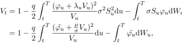
Lemma 2.2. The process V from equation (23) satisfies the BSDE V_t= 1 − q 2 Z _T t (ϕs+ λsVs)tr Vs dhM, M i_s(ϕ_s+ λ_sV_s) − Z _T t ϕtr_sdMs− (LT − Lt), (24)

where q := _γ−1γ . Moreover the optimal strategy is given by π_t∗= −x(F )(q − 1) µ ϕt V_t + λt ¶ E µ −(q − 1) Z _· 0 µ ϕu V_u + λu ¶_tr dSu ¶ t + ηt,

and the associated optimal wealth process Xx(F )_,π∗

by X_tx(F ),π∗ = x(F )E µ −(q − 1) Z _· 0 µ ϕu V_u + λu ¶_tr dSu ¶ t + Z _t 0 η_utrdSu,

where we denote the stochastic exponential by E ³ − (q − 1) Z _· 0 µ ϕu Vu + λu ¶_tr dSu ´ t= exp n − (q − 1) Z _t 0 µ ϕu Vu + λu ¶_tr dSu − (q − 1)2 2 Z _t 0 µ ϕu Vu + λu ¶_tr dhM, M iu µ ϕu Vu + λu ¶ o . Proof. By Lemma 2.1 we have to show that the optimization problem V (t, x) = (x(F )₎γ_V

tadmits

an optimal strategy ˜π∗ _{and that this optimal strategy can be characterized in terms of a BSDE.}

Since the power utility function satisfies the asymptotic elasticity condition, i.e. lim sup

x→∞

xU0_(x)

U (x) < 1,

the existence of an optimal strategy ˜π∗ _{is guaranteed (see e.g. [20]). Thus all the hypotheses}

of [22, Theorem 3.1 (or Theorem 4.1)] are satisfied, thus V is a solution of equation (24). Let Xx(F )_,˜_π∗

be the wealth process associated to the optimal strategy

˜ π_t∗ = argsup_π∈Π_˜ x(F )E "µ x(F )+ Z _T t ˜ πtr_udSu ¶γ¯_¯ ¯ ¯Ft # that is given by X_tx(F ),˜π∗ = x(F )+ Z _t 0 (˜π_u∗)trdS_u, t ∈ [0, T ]. By [22, Theorem 4.1] we have for t ∈ [0, T ]

X_tx(F ),˜π∗ = x(F )E µ −(q − 1) Z _· 0 µ ϕu Vu + λu ¶_tr dSu ¶ t , which implies ˜ π_t∗ = −x(F )(q − 1) µ ϕt V_t + λt ¶ E µ −(q − 1) Z _· 0 µ ϕu V_u + λu ¶_tr dSu ¶ t .

(16)

Then the identity π_t∗ = argsup_π∈Πη x(F ) E "µ x(F )+ Z _T t (πu− ηu)dSu ¶γ¯_¯ ¯ ¯Ft # = ˜π∗_t + ηt, t ∈ [0, T ],

yields the claim.

Obviously equation (24) has a unique solution by Proposition 1.3 because it belongs to the class of BSDEs of type (6).

Remark 2.3 (Mean variance hedging). If we consider higher values for γ, for instance if γ > 1, Lemma 2.2 (applied to −U ) still remains true. Observe that if γ = 2, there is a relationship between the mean variance hedging problem with a constant liability b > 0 and utility maxi-mization with respect to the utility function U (x) = 2bx − x2 _{= b}2_{− (x − b)}2 _{(see also section 4}

in [22]). More precisely, the problem of minimizing the hedging error via essinfπE h (x + Z _T t π_utrdSu− b)2 ¯ ¯Ft i is equivalent to maximizing esssup_πE h U (x + Z _T 0 πtrdS_u)¯¯F_t i = esssup_πE h 2b(x + Z _T 0 πtrdS_u) − (x + Z _T 0 πtrdS_u)2¯¯F_t i = b2− essinfπE h (x + Z _T 0 πtrdSu− b)2 ¯ ¯Ft i = b2− essinf_πE h (x − b)2 ³ 1 + Z _T 0 ¡ π x − b ¢_tr dS_u ´₂_¯ ¯F_ti = b2− (x − b)2Vt, where Vt = essinfπ˜E h³ 1 +R₀Tπ˜tr_dS u ´₂_¯ ¯Ft i = −esssup_˜_πE h − ³ 1 +R₀Tπ˜tr_dS u ´₂_¯ ¯Ft i satisfies the BSDE Vt= 1 − Z _T t (ϕs+ λsVs)tr V_s dhM, M is(ϕs+ λsVs) − Z _T t ϕtr_sdMs− (LT − Lt),

which is identical to equation (24) for q = 2. 2.1.2 Exponential utility

In this section we discuss the case where U (x) = −e−αx_{, x ∈ R, for some α > 0 is the exponential}

utility function. In [14] the optimization problem (20) has already been solved for general bounded liabilities. We extend some results by [14] by providing a solution for liabilities which are not necessarily bounded. Since this section has only a marginal connection to the BSDE (6), our approach is of rather illustrative character which is the reason to make a few simplifications: we assume throughout this section that we have dSt= σtdWt+ btdt where σ is a Rd×d-valued

non-negative adapted process, b is a Rd×1_{-valued adapted process and W denotes a d-dimensional}

Brownian motion. As a consequence, assuming that σσtr _{is invertible, we consider dM}

(17)

and λt:= (σtσtrt)−1btin (17). This dynamics of the price process basically creates the same setup

as in [14]. Note that the results presented here can be easily extended to the general continuous semimartingale setting. We refer to Section 2.2 where the approaches by Hu, Imkeller and M¨uller ([14]) and Morlais ([23] are described in a more general framework. Let us first recall the main result of [14] which considers bounded liabilities.

Bounded liability case: Let the liability F be a bounded F_T-measurable random variable satis-fying (21). Furthermore, assume the investor can only employ strategies π which belong to a closed set ˜C of Rd_{. Constraints on strategies appear often in reality and reflect e.g. regulations}

imposed by central authorities or company internal risk management policies. Note that this setting is a particular case of [14], and we refer the reader to it for considering a stock as a log normal type SDE. For convenience we let pt := πtrtσt (so that the constraint πt ∈ ˜C becomes

pt ∈ Ct with Ct := ˜Cσt). With this notation, we let Xtx,p := x +

R_t

0psdWs+

R_t

0psθsds with

θs:= σtrsλs. The set of admissible strategies for the investor is then given by

Πb := ½ p : Ω × [0, T ] → Rd: p (Ft) − adapted, E ·Z _T 0 |pu|2du ¸ < ∞, pt∈ Ct∀t ∈ [0, T ] ¾ . For this setting it has been shown in [14] that the optimization problem Vb_{(x), x > 0, defined}

by

Vb(x) := − sup

p∈Πb

E£exp¡−α(X_Tx,p− F )¢¤ admits at least one optimal p∗ _{such that every time t, p}∗

t is given as the projection of a process

Z_tb onto the set Ct, i.e. p∗t = proj(Ztb+θαt, Ct) where (Yb, Zb) denotes the unique solution of the

BSDE Y_tb = F − Z _T t (Z_sb)trdWs− Z _T t fb(s, Z_sb)ds, t ∈ [0, T ], (25) with fb_{(s, z) := −}α 2dist2 ¡ z + θs α, Cs ¢ + ztr_θ s+|θs| 2

2α , z ∈ Rd. In addition, the value function is

given by Vb_{(x) = − exp(−α(x − Y}b

0)), x > 0. Before turning to the unbounded case we state

two remarks which will be of importance in the following.

Remark 2.4. The existence and uniqueness of the BSDE (25) is due to the boundedness assumption on F , since the driver fb _{has quadratic growth in the z variable. Indeed a classical}

result from [19, Theorem 2.3] provides existence, while uniqueness has been proved in [14, Proof of Theorem 7].

Remark 2.5. Notably in the works [6] and [8], the boundedness condition on F has been relaxed to some exponential moment conditions which is essential to prove uniqueness of a solution. We refer to reader to [7] where uniqueness is proved for convex drivers (like the one we are considering) and to [1] where a number of counterexamples to uniqueness are constructed in the case f (z) = z2_.

Unbounded liability case: Assume that F is a square-integrable FT-measurable random variable

satisfying (21). Admissible strategies p will be understood as processes taking their values in a closed set Ct (again of the form ˜Cσt) in Rd at each time t. Since the liability is now unbounded

(and a priori can have infinite exponential moments), the investor’s strategies p are constrained to the set C_t+ η for every t. In other words, because of the unboundedness of F , the investor is allowed to escape the formal constraint sets Ct. Yet the escape is subject to an amount

determined by ηt. If the investor is a trader in a company, then one could see our setting

(18)

unbounded liability. Taking these remarks into account, we allow the set of admissible strategies to be given by Π := ½ p : Ω × [0, T ] → Rd: p (Ft) − adapted, E ·Z _T 0 |pu|2du ¸ < ∞, pt∈ Ct+ ηt∀t ∈ [0, T ] ¾ . We also introduce the set of strategies

˜ Π = Π − η := ½ ˜ p : Ω × [0, T ] → Rd: E ·Z _T 0 |˜pu|2du ¸ < ∞, ˜pt∈ Ct∀t ∈ [0, T ] ¾ . In this notation, the investor’s optimization problem is

V (0, x) := sup p∈Π E£− exp(−α(X_Tx,p− F ))¤ (26) = sup p∈Π E · − exp µ −α µ x(F )+ Z _T 0 (pu− ηu)trdSu ¶¶¸ = sup ˜ p∈ ˜Π E · − exp µ −α µ x(F )+ Z _T 0 ˜ ptr_udSu ¶¶¸ . (27)

In other words, one can replace an optimization problem of type (26) that has a liability F and trading restrictions given by Π by an optimization problem of type (27) that has no liability but trading restrictions translated by η, the replication process of F .

Lemma 2.6. Let F be square integrable liability as above. Then an optimal strategy p∗ of (26) is such that p∗

t = proj(ZtF− ηt+θ_αt, Ct) + ηt, t ∈ [0, T ], where (YF, ZF) is the unique solution of

the BSDE Y_tF = F − Z _T t (Z_sF)trdWs− Z _T t fF(s, Z_sF)ds, t ∈ [0, T ], (28) with fF_{(s, z) := −}α 2dist2 ¡ z − ηs+θ_αs, Cs ¢ +|θs|2 2α + (ztr− ηs)θs, s ∈ [0, T ], z ∈ Rd.

Proof. Before entering into the details note that the driver of BSDE (28) is quadratic in z. From the literature we know that existence and uniqueness of solutions for such a BSDE are ensured if the terminal condition F is bounded or has at least finite exponential moments. Here we are able to show existence and uniqueness without this assumption. This is due to the particular form of the driver which in a sense takes into account the terminal condition F . We refer the interested reader to Remark 2.7.

It is shown in [14, Theorem 7] that a solution ˜p∗ of (27) exists and is given as the projection of Z0 _{on the set C, i.e. ˜}_p∗

t := proj(Zt0+θαt, C) where (Y0, Z0) is solution of the BSDE

Y_t0 = 0 − Z _T t (Z_s0)trdWs− Z _T t f0(Z_s0)ds (29) with f0_{(s, z) := −}α 2dist2 ¡ z +θs α, Cs ¢ + ztr_θ s+|θs| 2

2α . From the classical result of [19, Theorem

2.3] the BSDE (29) admits at least a solution, and by the proof of [14, Theorem 7] uniqueness is guaranteed. Since ˜Π = Π − η we get from Theorem 2.1 that p∗ _{:= ˜}_p∗_{+ η = proj(Z}0₊θ

α, C) + η is

an optimal strategy for (27). Existence and uniqueness of the solution of BSDE (29) will imply that a unique solution of (28) exists and is given by YF _{= Y}0₊R·

0ηudWu and ZF = Z0+ η.

Indeed let U := Y0

t +

R_·

0ηudWu and V := Z0+ η. Then equation (29) implies

Ut = F − Z _T t V_strdWs− Z _T t f0(Z_s0)ds = F − Z _T t V_strdWs− Z _T t fF(s, Vs)ds, t ∈ [0, T ],

(19)

where the last equality comes from the fact that fF(s, Vs) = −α₂dist2 µ Z_s0+θs α, Cs ¶ +|θs|2 2α + (Z 0 s)trθs = f0(s, Zs0), ∀s ∈ [0, T ].

This proves that a solution of (28) exists. Its uniqueness is a direct consequence of the previous computation and the uniqueness of the solution of BSDE (29).

Remark 2.7. As a byproduct, we get that the quadratic BSDE (28) admits a unique solution with terminal condition F which is neither assumed to be bounded nor to have finite exponential moments. To our knowledge, this is the first example of such a BSDE. Obviously the quadratic driver fF _{has a special form, since it contains in a sense the terminal condition F via the}

predictable process η. This type of driver escapes and complements the analysis of [6, 8].

2.2 Multiplicative liability for power utility

In this section we derive a BSDE for solving (19) in case U is the power utility function U (x) = xγ_{, x > 0, with γ ∈ (0, 1). Our objective now is to solve the optimization problem}

V (0, x) = sup

π∈ΠxE

£

(X_Tx,π)γFγ¤ (30)

with Xx,π _{given by (18) and F being an F}

T-measurable random variable satisfying 0 < F < 1.

Note that such liabilities assess the wealth of the investor by a random portion at maturity T > 0. One can think of F as some portion of charges or tax rates which are subject to external fluctuations. In order to solve (30), let ¯ρi

tbe the part of the wealth invested in the i-th stock at

time t. We denote ρi_t = ρ¯it Si

t and by ρ we denote the vector in R

d×1 _{with ith component ρ}i _for

i = 1, . . . , d. With this parametrization of the strategies, the wealth process satisfies X_tx,ρ= x + Z _t 0 X_ux,ρρudSu = x exp µZ _t 0 ρtr_udSu−1₂ Z _t 0 ρtr_udhM, M iuρu ¶ , t ∈ [0, T ]. We assume that our investor has to face some trading constraints (coming for example of a general regulations institution) modeled by a closed, not necessarily convex set C in Rd. The set of admissible strategies is then given by the square integrable stochastic processes (ρt)t∈[0,T ]

such that ρt belongs P-almost surely to C for every t. As a consequence, (30) becomes

V (0, x) = sup ρ∈ΠC E · xγexp µ γ Z _t 0 ρtr_udS_u−γ 2 Z _t 0 ρtr_udhM, M i_uρ_u ¶ Fγ ¸ (31) with ΠC := ½ ρ : Ω × [0, T ] → R, Z _T 0 ρtr_udhM, M iuρu< ∞, ρt∈ C, ∀t ∈ [0, T ], P − a.s. ¾ . Our approach to solve (30) is a straightforward modification of the computations from [14, Section 3] (see also [23] for the continuous martingale setting). We nevertheless reproduce their essential elements for the comfort of reading. The key ingredient of martingale optimality comes in the task of finding a family of stochastic processes Rx,ρ _{such that}

1. Rx,ρ_T = U (X_Tx,ρF ), for all ρ in Πx,

(20)

3. Rx,ρ _{is a supermartingale for all ρ in Π}

x and there exists an element ρ∗ in Πx such that

Rx,ρ∗

is a martingale.

The formulation of the problem in (31) suggests that the process R is of the form Rx,ρ_t := xγexp µ γ Z _t 0 ρtr_udS_u−γ 2 Z _t 0 ρtr_udhM, M i_uρ_u ¶ exp(Y_t), where Y solves a BSDE

Y_t= γ log(F ) − Z _T t Z_strdM_s− Z _T t f (s, Z_s)dK_s− Z _T t dL_s+1 2 Z _T t dhL, Li_s, (32) with a driver f to be determined. In this way Rx,ρ _{can be rewritten as}

R_tx,ρ= xγexp(Y0)E µZ _· 0 (γρu+ Zu)trdMu+ Lt ¶ t exp (I_txρ) . Recalling dhM, M it= σtσtrtdKt, we have I_txρ:= Z _t 0 · 1 2|σ tr u (γρu+ Zu) |2− γ₂|σtruρu|2+ γ(ρtruσuσutrλu) + f (u, Zu) ¸ dKu, t ∈ [0, T ].

Now martingale optimality requires to look for drivers f such that for every ρ we have 1

2|σ

tr

u (γρu+ Zu) |2−γ₂|σutrρu|2+ γ(ρtruσuσutrλu) + f (u, Zu) ≤ 0, ∀u ∈ [0, T ], (33)

and such that there exists a ρ∗ for which the inequality above becomes an equality. According to (33) we need f (u, Zu) ≤ γ(1 − γ) 2 ¯ ¯ ¯σ_utrρu− σtr u(Zu+ λu) 1 − γ ¯ ¯ ¯2− γ 2(1 − γ)|(Zu+ λu) tr_σ u|2− 1 2|σ tr uZu|2, which leads to f (u, z) = γ(1 − γ) 2 dist 2³ σutr(z + λu) 1 − γ , ˜Cu ´ − γ 2(1 − γ)|(z + λu) tr_σ u|2−1₂|σtruz|2, (34) where ˜Cu := σtruC, and dist2³ (z + λu) 1 − γ , ˜Cu ´ := min ˜ ρu∈ ˜Cu ¯ ¯ ¯˜ρ_u−σutr(Zu+ λu) 1 − γ ¯ ¯ ¯2, u ∈ [0, T ], z ∈ Rd.

Then the optimal ρ∗ _{is given by ˜}_ρ∗ _{= σ}tr_ρ∗ _{with ˜}_ρ∗ _{an element realizing the distance above.}

More specifically, we have

ρ∗ = (σσtr)−1σtrρ˜∗.

Remark 2.8. Note that if no constraints are imposed on the strategies (i.e. C = Rd_{), then the}

driver of equation (34) becomes f (u, z) = − γ 2(1 − γ)|(z + λu)σu| 2₋1 2|σ tr uz|2, u ∈ [0, T ], z ∈ Rd.

(21)

3 Numerical simulation of utility maximization problems

To illustrate the two step algorithm presented in the preceding sections, we now provide two numerical examples on solving the additive and multiplicative maximization problem with re-spect to the power utility function. As [14] shows, optimization problems with rere-spect to the exponential utility function without constraints lead to linear BSDE right away, and thus offer an immediate access for numerical simulation. We conclude with an example in which we con-strain strategies to integer values. The resulting nonlinear BSDE is numerically tractable. Its simulations are curiously close to the ones for the corresponding unconstrained BSDE.

3.1 Example for the additive power utility case

Recall the additive optimization problem from Section 2.1.1,

V (0, x) = sup π∈Πηx E "µ x + Z _T 0 πtr_udSu− F ¶γ# ,

where x > 0 denotes the initial capital, γ ∈ (0, 1) denotes the risk aversion parameter and the FT-measurable bounded liability F satisfies F = c +

R_T

0 ηudSu for a constant c > 0 and

a predictable process η. We consider a one-dimensional Black-Scholes market composed by a

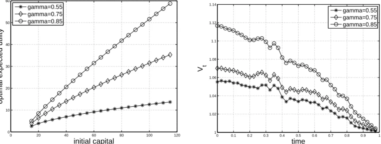
0 20 40 60 80 100 120 0 10 20 30 40 50 60 initial capital

optimal expected utility

gamma=0.55 gamma=0.75 gamma=0.85

(a) Optimal expected utility V (0, x) in dependence of the initial capital x.

0 0.1 0.2 0.3 0.4 0.5 0.6 0.7 0.8 0.9 1 1 1.02 1.04 1.06 1.08 1.1 1.12 1.14 time V t gamma=0.55 gamma=0.75 gamma=0.85

(b) Pathwise supermartingale property of the BSDE value process V .

Figure 1: Optimal expected utility and pathwise supermartingale plot. stock and a zero interest rate bank account. The stock evolves according to

dSt= σStdWt+ µStdt

where µ ∈ R and σ ∈ R+ are the constant drift and volatility coefficients. This choice implies

that dMt= σStdWt and λ_t= µSt σ2_S2 t = µ σ2S −1 t . (35)