Assessment of the impact of the measurement precision of thermal properties of materials on the prediction of their thermal behaviour

(1)

SHERBROOKE

Faculte de genie

Departement de genie mecanique

Assessment of the Impact of the Measurement Precision of Thermal

Properties of Materials on the Prediction of Their Thermal Behaviour

r

(Evaluation de l'impact de la precision de mesure des proprietes thermiques des

materiaux sur la prediction de leur comportement thermique)

Memoire de maitrise

Speciality: Genie Mecanique

Ayesha KHATUN

Jury:

Prof. Martin Desilets, PhD (directeur)

Prof. Gervais Soucy, PhD

Prof. Said Elkoun, PhD

(2)

1+1

Published Heritage Branch Direction du Patrimoine de I'edition 395 Wellington Street Ottawa ON K 1A0N 4 Canada 395, rue Wellington Ottawa ON K1A 0N4 Canada

Your file Votre reference ISBN: 978-0-494-96269-5 Our file Notre reference ISBN: 978-0-494-96269-5

NOTICE:

The author has granted a non

exclusive license allowing Library and Archives Canada to reproduce, publish, archive, preserve, conserve, communicate to the public by

telecomm unication or on the Internet, loan, distrbute and sell theses

worldwide, for commercial or non commercial purposes, in microform, paper, electronic and/or any other formats.

AVIS:

L'auteur a accorde une licence non exclusive permettant a la Bibliotheque et Archives Canada de reproduire, publier, archiver, sauvegarder, conserver, transmettre au public par telecomm unication ou par I'lnternet, preter, distribuer et vendre des theses partout dans le monde, a des fins com merciales ou autres, sur support microforme, papier, electronique et/ou autres formats.

The author retains copyright ownership and moral rights in this thesis. Neither the thesis nor substantial extracts from it may be printed or otherwise reproduced without the author's permission.

L'auteur conserve la propriete du droit d'auteur et des droits moraux qui protege cette these. Ni la these ni des extraits substantiels de celle-ci ne doivent etre imprimes ou autrement

reproduits sans son autorisation.

In compliance with the Canadian Privacy A ct some supporting forms may have been removed from this thesis.

W hile these forms may be included in the document page count, their removal does not represent any loss of content from the thesis.

Conform em ent a la loi canadienne sur la protection de la vie privee, quelques

form ulaires secondaires ont ete enleves de cette these.

Bien que ces form ulaires aient inclus dans la pagination, il n'y aura aucun contenu manquant.

(3)

ABSTRACT

The thermal properties o f the sidewall lining materials are capturing attention since the last two decades. Good prediction o f the dynamic thermal behaviour o f Hall Heroult cells, including precise estimation o f energy losses and location o f the side ledge formed by the solidification of electrolytic bath, is made possible when the sidelining materials are well characterized in function o f temperature. The present work aim at measuring the thermal diffusivity, heat capacity and thermal conductivity o f silicon carbide (SiC), graphitic and graphitized carbon materials and cryolite (NasAlFe) based on transient characterization techniques. The thermal diffusivity and the heat capacity are measured by using state-of-the-art transient laser flash analyzer and differential scanning calorimeter respectively. The thermal conductivity is calculated by assuming a constant density.

The range o f precision error for each thermal property is also calculated for a finite number of data sets. Empirical correlation has been drawn for each o f the properties to describe the relation with temperature in mathematical terms. Thermal characterization o f the latent heat evolved during the melting o f ledge is also carried out. Finally, based on the calculations conducted with a 2-D numerical model, the effect o f the precision errors o f temperature varying thermal properties of the sidewall materials and ledge on the dynamic behaviour o f a laboratory scale phase change reactor is also presented.

The results, so obtained, encourage further studies on the thermal properties o f materials used in the aluminium reduction cell to find out the thermal environment inside the cell, heat loss estimation and effect o f the additives on the location o f ledge.

Key words: Thermal conductivity, thermal diffusivity, heat capacity, temperature varying properties, precision error, phase change profile, latent heat.

(4)

RESUME

Les proprietes thermiques des materiaux utilisees pour la construction des murs lateraux d ’une cuve d ’electrolyse de l ’aluminium captent l ’attention depuis les deux demieres decennies. Une bonne prediction du comportement thermique dynamique des cellules Hall-Heroult, y compris une estimation precise des pertes d'energie et de l'emplacement du gel sur le cote, est rendue possible lorsque les materiaux de cote sont bien caracterises en fonction de la temperature. L'objectif de ce travail consiste a mesurer la diffusivity thermique, la capacite calorifique et la conductivity thermique du carbure de silicium, des materiaux carbones du cote (graphitique et graphitise) et de la cryolite a l’aide de techniques de caracterisation transitoires. La diffusivity thermique et la capacite de calorifique sont mesurees en utilisant respectivement un diffixsivimetre thermique et un calorimetre a balayage differentiel. La conductivity thermique est calculee en supposant une masse volumique constante.

La marge d'erreur sur la precision de chaque propriety thermique a egalement ete calculee pour un nombre fini d'ensembles de donnees. Une conflation empirique a ete elaboree pour chacune des propriytys pour dycrire la relation avec la temperature en termes mathematiques. La caracterisation thermique de la chaleur latente degagee lors de la fonte de la gelee de cote est egalement effectuee. Enfin, sur la base des calculs effectues avec un modele 2-D numerique, l'effet des erreurs de mesure entachant les differentes proprietes thermiques des materiaux du cote sur le comportement dynamique d'un reacteur a changement de phase de type laboratoire est ygalement presente.

Les rysultats obtenus montrent l’interet de nouvelles etudes sur les propriytes thermiques des materiaux utilises dans les cellules d ’electrolyse de l'aluminium pour decouvrir 1’influence de

l'environnement thermique interieur de la cellule, pour estimer les pertes de chaleur et l'effet des additifs sur l’emplacement du front de solidification.

Mots-ciys: Conductivity thermique, diffusivite thermique, capacite calorifique, erreur de mesure, profil de gelee, chaleur latente.

(5)

My mother Shahida Begum, brother Foezur Rahman Chowdhury and my Professor

(6)

ACKNOWLEDGEMENT

I would like to express my deepest sense o f appreciation, gratitude and indebtedness to my honorable supervisor Professor Martin Desilets for giving me the opportunity o f being a part of his research team. My heartiest gratitude and thanks to Prof. Desilets who gave me the chance and honor to be associated with his research, which opens a new window in my career. I greatly appreciated his continuous support, excellent supervision and encouragement throughout the project.

Thanks to Rio Tinto Alcan group for supporting and funding my thesis project. It sure will help me to conduct a bright future career. I would like to express my gratitude to Rio Tinto Alcan for providing their support for my project and introduced me with the new research world of aluminium.

I want to give special thanks to Mr. Serge Gagnon and Mr. Francis Barrette who provided a great support in my experimental work. It is also a pleasure for me to express my sincere appreciation and profound regards to NETZSCH technical staff for providing the guidelines to efficiently conduct and analyzed all the experimental works.

I would like to give thanks to Mr. Marc-Andre Marois and Mr. Clement Bertrand who all time gave me their helping hands to conduct my research work. Thanks to both o f them for their contribution and suggestions to accomplish my research work.

I wish to thank all the staff o f the Mechanical Engineering department for their valuable support. I also would like to acknowledge my colleagues Ms.Carine Havet, Mr. Mohammed Khennich, Mr. James Christopher Reddick and Mr. Jean-Sebastien Savard for their contributions, suggestions and friendship during the courses.

And last but not the least, I profoundly acknowledge gratefulness to my beloved brothers, sisters and sister-in-law who have provided me constant encouragement.

(7)

LIST OF FIGURES

Figure 1.1: A typical Hall-Heroult Cell [Li et al., 2009]... 1 Figure 1.2: Typical heat losses from pot areas as a percentage o f the total pot heat losses [Bruggeman, 1998]... 3 Figure 1.3: Precision error during the measurement o f thermophysical properties o f refractory material...4 Figure 3.1: Layout o f the sidewall region o f an aluminium cell...7 Figure 3.2: Temperature profile through a horizontal section o f the sidewall for one dimensional, steady state heat loss [Bruggeman, 1998]...8

Figure 3.3: Example o f a vertical heat flux profile measured on the sidewall o f a pot [Bruggeman, 1998]... 9 Figure 3.4: Variation o f the ledge thickness associated with alumina feeding for the bath/ledge heat transfer coefficient of 830 W/m2K [Wei et al., 1997]...10 Figure 3.5: Heat loss mechanisms in zone A and B [McFadden, 1998]... 10 Figure 3.6: A schematic o f multilayer cell wall including side ledge [Barantsev et al.,

2000] 12

Figure 3.7: Variation of the ledge thickness for acidic bath after charging 200 kg A1F3

[Barantsev et al., 2000]...12 Figure 3.8: Temperature distribution in the carbon block and the ledge at the bath zone [Yurkov et Mann, 2005]... 13 Figure 3.9: Bath ledge thickness evolution using ANSYS® 2D+ dynamic model 14 Figure 3.10: Computational domain including a part o f the sidewall carbon block and the ledge solidified over it [Boily etal., 2001]... 14 Figure 3.11: Identified interfaces and measured interfaces for a) uniform, b) sloped and c) wedge-shaped sand layer [Boily et al., 2001]... 16 Figure 3.12: Relative variation o f the interface position in function o f the variation o f the thermal conductivity o f sidewall block [Boily et al., 2001]...16 Figure 3.13: Thermal resistance network with two heat flow channels [Kiss et Dassylva, 2008]... 17

(12)

Figure 3.14: Computed ledge profiles corresponding to different heat inputs in term o f the

nominal power [Kiss and Dassylva, 2008]... 18

Figure 3.15: Variation o f the average thickness o f the ledge as function o f the heat input [Kiss et Dassylva, 2008]... 18

Figure 3.16: A schematic o f the thermal reactor [Marois et al., 2009]... 20

Figure 3.17: Thermal conductivity o f different cathode blocks (along grain direction) as a function o f temperature [Dumas et Lacroix, 1994: Lombard et al., 1998]...23

Figure 3.18: Thermal conductivity o f used cathode bottom blocks o f amorphous type as a function o f temperature [Sorlie et al., 1995]...24

Figure 3.19: Thermal conductivity o f different grade o f graphite cathode blocks as a function o f temperature [Allard et al., 2000]... 25

Figure 3.20: Temperature dependence o f the thermal diffusivity o f SiC ceramics [Liu et Lin, 1995]... 26

Figure 3.21: Temperature dependence o f the thermal conductivity o f SiC ceramics [Liu et Lin, 1995]... 27

Figure 3.22: SEM image o f Si3N4-SiC refractory [Pan et al., 2009]... 28

Figure 3.23: Thermal conductivity o f Si3N4-SiC refractory [Pan et al., 2009]... 28

Figure 4.1: Laser flash method, (a) Laser applied at the front side o f the sample, (b) Principle o f the laser flash method [Czichos et al. ,2006]... 30

Figure 4.2: Furnace o f the heat flux differential scanning calorimeter [Czichos et al., 2006]. ... 32

Figure 4.3: Ledge collected from the aluminium cell... 34

Figure 4.4: SiC block collected from the aluminium cell sidewall... 34

Figure 4.5: Graphitized carbon block collected from the aluminium cell... 35

Figure 4.6: Graphitic carbon block collected from the aluminium cell... 35

Figure 4.7: Concrete HS and brick K26 at the bottom (exposed surface) o f the oven 36 Figure 4.8: Kaowool blanket used at the sidewall o f the oven... 37

Figure 4.9: First step o f heat capacity measurement sample preparation (Cylinder preparation)...38

(13)

Figure 4.10: Diamond saw...39

Figure 4.11: First step o f thermal diffusivity measurement sample preparation (cylinder preparation): graphitized carbon cylinders...40

Figure 4.12: Second step o f the thermal diffusivity measurement samples preparation (sample slicing)... 42

Figure 4.13: Sample thickness reduction o f the solid bath... 43

Figure 4.14: Sketch o f the sample coated by two graphite layers... 43

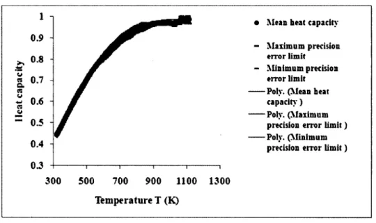
Figure 5.1: Precision error interval for the heat capacity o f graphitic carbon... 48

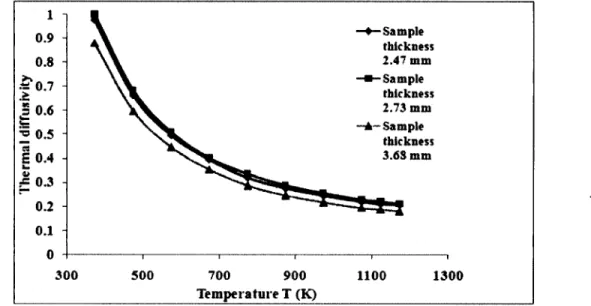
Figure 5.2: Thermal diffusivity o f graphitic carbon for three different sample thicknesses. ... 49

Figure 5.3: Precision error interval for the thermal diffusivity measurement o f graphitic carbon... 50

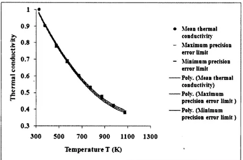
Figure 5.4: Precision error interval for the thermal conductivity of graphitic carbon 52 Figure 5.5: Precision error interval for the heat capacity measurement o f graphitized carbon... 53

Figure 5.6: Thermal diffusivity for three different sample thicknesses o f graphitized carbon. ... 54

Figure 5.7: Precision error for the thermal diffusivity o f graphitized carbon...55

Figure 5.8: Precision error for the thermal conductivity o f graphitized block... 56

Figure 5.9: Precision error interval for the heat capacity o f SiC... 58

Figure 5.10: Thermal diffusivity for three different sample thickness o f SiC...59

Figure 5.11: Precision error for the thermal diffusivity of SiC...59

Figure 5.12: Precision error for the thermal conductivity o f SiC... 61

Figure 5.13: Precision error for the heat capacity o f ledge... 63

Figure 5.14: Ledge samples prepared for the thermal diffusivity measurements... 64

Figure 5.15: Comparison o f the thermal diffusivity o f the ledge according to the sample production methods...65

(14)

Figure 5.16: Comparison o f the thermal conductivity o f the ledge according to the sample production methods...65 Figure 5.17: Thermal diffusivity o f the ledge for three different sample thicknesses 6 6

Figure 5.18: Precision error for the thermal diffusivity for ledge... 67 Figure 5.19: Precision error interval for the thermal conductivity of ledge...6 8

Figure 5.20: Latent heat o f ledge... 71 Figure 6.1: Schematic o f the thermal reactor represented by the mathematical model developed... 73 Figure 6.2: Schematic o f the thermal reactor for modified mathematical model...74 Figure 6.3: Treatment o f the irregular geometry (a) Real domain (irregular shape) (b) Nominal domain (regular shape)...77 Figure 6.4: Discretized control volumes in axis-symmetric coordinate over the whole calculation domain o f the experimental bench...77 Figure 6.5: Internal control volume for two-dimensional axis-symmetric coordinate 79 Figure 6.6: Structure o f the computer program of described numerical model...83

Figure 6.7: Flow diagram o f the computer program...84 Figure 6.8: Prediction o f solidification front o f teflon at steady state conditions for different

meshes at time step 1 0 s...8 6

Figure 6.9: Prediction of the solidification front o f teflon at steady state conditions at different time steps for spatial mesh 0.005 m in both r and y axis...8 6

Figure 6.10: Evaluation o f the energy imbalance at different time steps for spatial mesh 0.005 m in both r and y axis during teflon solidification process...87 Figure 6.11: Effect o f the time steps on the average progression o f the solidification front 6

h after starting the solidification process o f teflon for spatial mesh 0.005 m in both r and y axis...87 Figure 6.12: Crucible filled with liquid teflon before starting the solidification process [Coulombe, 2009]... 89 Figure 6.13: Measured T/Cl and T/C2 before starting the solidification process o f teflon. 90

(15)

Figure 6.14: Calculated T/Cl and T/C2 before starting the solidification process o f teflon. ... 91 Figure 6.15: Measured temperature T/Cl during the whole solidification process o f teflon. ... 91 Figure 6.16: Calculated temperature T/Cl during the solidification process o f teflon 92 Figure 6.17: Measured temperature T/C2 4 h after starting the solidification process o f teflon... 92 Figure 6.18: Calculated temperature T/C2 4 h after starting the solidification process o f teflon... 93 Figure 6.19: Solidification front thickness as a function o f time at the inner bottom centre o f the crucible... 93 Figure 7.1: Initial temperature profile o f the whole experimental bench before starting the solidification process... 95 Figure 7.2: Prediction o f the solidification front o f teflon at steady state conditions 97 Figure 7.3: Temperature profile o f the whole oven for teflon solidification process at steady state conditions... 97 Figure 7.4: Power losses through the oven during the solidification process o f teflon 98 Figure 7.5: Effect of the heat input on the prediction o f the solidification front profile of teflon at steady state conditions... 99 Figure 7.6: Effect o f the heat input on the prediction o f the transitory behaviour o f the average solidification front o f teflon in the crucible...1 0 0

Figure 7.7: Effect o f the forced convection heat transfer coefficient on the prediction o f solidification front profile o f teflon at steady state conditions...1 0 0

Figure 7.8: Effect o f the forced convection heat transfer coefficient on the transitory behaviour of the average solidification front o f teflon in the crucible...1 0 1

Figure 7.9: Effect o f the temperature difference between softening point and liquefaction temperatures on the prediction o f the solidification front o f teflon at steady state conditions.

:

101

Figure 7.10: Effect o f the temperature difference between softening point and melting temperatures on the prediction o f the transitory behaviour o f solid front o f teflon 1 0 2

(16)

Figure 7.11: Effect o f the precision error o f the thermal conductivity o f brick K26 on the prediction o f the solidification front o f Teflon at steady state conditions...102 Figure 7.12: Effect o f the precision error o f the thermal conductivity o f concrete HS on the prediction o f the solidification front o f teflon at steady state conditions... 103 Figure 7.13: Effect o f the thermal conductivity of solid teflon on the prediction o f the solidification front at steady state conditions... 104 Figure 7.14: Effect o f the thermal conductivity of solid teflon on the prediction o f the transitory behaviour o f the solidification front o f teflon... 104 Figure 7.15: Effect of the thermal conductivity o f liquid teflon on the prediction o f the solidification front o f teflon at steady state conditions...105 Figure 7.16: Effect o f the thermal conductivity o f liquid teflon on the transitory behaviour o f the average solidification front in the crucible... 105 Figure 7.17: Temperature profile o f the whole experimental bench before starting the solidification process o f liquid electrolytic bath... 107 Figure 7.18: Progression o f the solidification front with time at the centre o f the crucible during the solidification process o f liquid electrolytic bath... 107 Figure 7.19: Temperature profile o f the whole experimental bench at steady state conditions for the solidification process o f liquid electrolytic bath...108 Figure 7.20: Power losses through the oven during the solidification process o f liquid electrolytic bath... 1 1 0

Figure 7.21: Effect o f the input heat flux on the prediction o f the solidification front o f ledge at the steady state conditions...1 1 1

Figure 7.22: Effect o f the input heat flux on the prediction on the transitory behaviour o f the average solidification front o f ledge... :...1 1 1

Figure 7.23: Thermal resistances on the constant heat flow path from oven to ambient region...1 1 2

Figure 7.24: Effect o f the forced convection heat transfer coefficient on the prediction of the solidification front o f ledge at steady state conditions... 113 Figure 7.25: Effect o f the forced convection heat transfer coefficient on the prediction o f the transitory behaviour o f ledge...113

(17)

Figure 7.26: Effect o f the temperature difference between solidus and liquidus temperature o f bath on the prediction o f the ledge at steady state conditions... 114 Figure 7.27: Effect o f the difference between solidus and liquidus temperature o f bath on the prediction o f the transitory behaviour o f the average thickness o f ledge...114 Figure 7.28: Effect o f the sidewall lining materials on the prediction o f thickness o f ledge at steady state conditions... 116 Figure 7.29: Effect o f the sidewall materials on the transitory behaviour of the average thickness o f ledge... 117 Figure 7.30: Effect o f the precision error of the thermal conductivity o f graphitic carbon on the prediction o f the solidification front o f ledge at steady state conditions...117 Figure 7.31: Effect o f the precision error o f the thermal conductivity o f graphitic carbon on the transitory behaviour o f ledge...118 Figure 7.32: Effect o f the precision error o f the thermal conductivity o f graphitized carbon on the prediction of the solidification front o f ledge at steady state conditions... 118 Figure 7.33: Effect o f the precision error o f the thermal conductivity o f graphitized carbon on the transitory behaviour o f ledge...119 Figure 7.34: Effect o f the precision error o f the thermal conductivity o f SiC on the prediction o f ledge thickness at steady state conditions... 119 Figure 7.35: Effect of the precision error o f the thermal conductivity o f SiC on the transitory behaviour o f average thickness o f ledge...1 2 0

Figure 7.36: Effect o f the measurement precision of ledge thermal conductivity on the prediction o f solidification front o f ledge at steady state conditions...1 2 2

Figure 7.37: Effect o f the ledge thermal conductivity on the transitory behaviour o f average thickness o f ledge...1 2 2

Figure 7.38: Effect o f the thermal conductivity o f liquid bath on the prediction o f the solidification front o f ledge at steady state conditions... 123 Figure 7.39: Effect o f the thermal conductivity o f liquid bath on the transitory behaviour of the average thickness o f ledge...123 Figure A l: Semi quantitative analysis o f the solid cryolite... 128 Figure B1: Precision error interval for the heat capacity o f brick K 2 6 ... 129

(18)

Figure B2: Precision error interval for the thermal diffusivity o f brick K26...130

Figure B.3: Precision error interval for the thermal conductivity o f brick K 2 6 ... 131

Figure B.4: Precision error interval for the heat capacity o f concrete H S ...132

Figure B.5: Precision error interval for the thermal diffusivity o f concrete H S ... 133

Figure B.6: Precision error interval for the thermal conductivity o f concrete H S, 134 Figure B.7: Precision error interval for the heat capacity o f teflon... 136

Figure B.8: Latent heat evaluation o f teflon... 137

Figure B.9: Precision error interval for the heat capacity measurement o f zinc... 137

Figure B.10: Precision error interval for the thermal diffusivity of zinc... 138

Figure B.l 1: Precision error interval for the thermal conductivity o f zinc...140

Figure B.12: Latent heat evaluation o f zinc... 141

Figure B.13: Three repeated measurements o f the thermal diffusivity o f led g e... 144

Figure B.14: Three repeated measurements o f the thermal conductivity o f ledge 145 Figure C. 1: Treatment o f the boundary control volum e... 143

Figure C.2: Comer control volume...146

Figure C.3: Treatment o f the non-uniform thermal conductivity for 2-D control volume 149 Figure D .l: Energy compensation during the solidification o f the teflo n... 151

Figure D.2: Average progression o f the solidification front o f teflon with tim e... 151

Figure D.3: Variation o f the maximum temperature difference between two meshes with time in the solidification process o f teflon... 152

Figure D.4: Location o f the maximum temperature difference at steady state o f solidification process o f teflon... 152

Figure D.5: Power accumulation of the oven during the solidification process o f liquid electrolytic bath... 153

Figure D.6: Prediction o f the solid front of ledge at steady state conditions...153

(19)

Figure D.8: Variation o f maximum temperature in the oven from one iteration to another

iteration in the solidification process o f liquid bath...154 Figure D.9: Location o f the maximum temperature difference at steady state of solidification process o f liquid bath...155

(20)

LIST OF TABLES

Table 3.1: Bath and cryolite ratio [Grjotheim et Kvande, 1993]...20

Table 3.2: Variation of the ledge thickness according to AI2O3 (wt %) and AIF3 (wt %).21 Table 3.3: Concentration (in volume percent) of SiC polytypes for A-, B-, C-and D- SiC starting materials (Raw) and after hot-pressed sintering (HP) [Liu et Lin, 1995]... 26

Table 4.1: Elemental analysis o f the ledge...34

Table 4.2: Image o f the heat capacity measurement samples...39

Table 4.3: Mass o f the heat capacity measurement samples...39

Table 4.4: Ideal thickness of the thermal diffusivity measurement samples [Netzsch laser flash analyzer instrument manual, 2009]... 41

Table 4.5: Thickness o f the prepared thermal diffusivity measurement samples... 41

Table 5.4: Density o f sintered bonded silicon carbide [NIST, 2010]...51

Table 5.17: Different parameters affecting the thermal diffusivity o f ledge... 64

Table 5.20: Composition o f used ledge [Rio Tinto Alcan]...69

Table 6.1: Comparison of numerical results with experimental results...90

Table 7.1: Physical data used in the numerical calculations o f phase change problem o f teflon... 96

Table 7.2: Power losses estimation o f the whole oven at steady state conditions o f the solidification process o f teflon... 98

Table 7.3: Physical data used in the numerical calculations o f the phase change problem o f liquid electrolytic bath...109

Table 7.4: Power losses distribution in the oven at the steady state conditions of the solidification process of liquid electrolytic bath...1 1 0 Table 7.5: Power losses estimation for three different sidewall lining materials at the steady state conditions for the solidification process o f liquid electrolytic bath 116 Table B. 1: Precision error interval for the heat capacity o f brick K 26... 129

(21)

Table B.3: Precision error interval for the thermal conductivity o f brick.K26...131

Table B.4: Precision error for the heat capacity o f concrete H S ...133

Table B.5: Precision error interval for the thermal diffusivity o f concrete H S ...134

Table B.6: Precision error for the thermal conductivity o f concrete... 135

Table B.7: Precision error for the heat capacity o f T eflon... 136

Table B.8: Precision error for the heat capacity of z in c ... 138

Table B.9: Precision error for the thermal diffusivity of zinc...139

(22)

LIST OF SYMBOLS

Symbols Definition Units

a Thermal resistance at the boundary of

the control volume K/W

A Surface area m2

Cp Heat capacity J/kg/k

dy Discretized mesh distance in y direction m

/ Liquid fraction

h Heat transfer coefficient W/m2/K

lh Latent heat J/kg

L Radius o f the oven m

Lby Thickness o f the brick K26 layer

at the bottom o f the oven m

Lcruy Height o f the crucible m

Lcy Thickness o f the concrete HS

layer at the bottom o f the oven m

Ly Height o f the oven m

mr Molar ratio

M Mass kg

M_r Total number o f meshes in the radial direction o f the oven

(23)

of the sand layers

-qH , q K Heat flow at Ti and / j boundary J

Q Heat flow J

r Radius o f the boundary o f the control

volume m

R Thermal resistance KAV

Rs Deviation o f the fitted data from the

measured data

-t Time s

T Temperature K

TT2>Tr2

Temperature at the T2 and T3 boundary K

X Thickness m G reek letters a Thermal diffusivity m2/s SH Change o f enthalpy J/kg A T Temperature difference K X Thermal conductivity W/m/K P Density kg/m3

0 Temperature o f the annulus K

Subscripts

amb Ambient

(24)

b f Brick inner surfaces (east)

bl Ledge contacting with liquid electrolytic bath bs South side surface o f brick K26

B Liquid electrolytic bath to ambient without ledge

c Crucible

cc Contacting surface between the components o f furnace sidewall

co Crucible outer surface

c f Concrete inner surface (east)

cw Carbon wall

cwl Contact point between carbon sidewall and ledge

e East side

/ Forced convection

f t Ledge

f r Furnace wall components

i Inner

/ Liquid PCM

liq Liquidus

l-b Ledge at the liquid electrolytic bath region

m Molten aluminium

ml Molten aluminium and liquid electrolytic bath

n North side

(25)

0 Outer

ov Oven

p Current mesh

so Solid PCM

s, south South side

sil Steel, insulation and ledge

sh Steel shell

si Solidus

Sai Contact point between ledge and liquid bath

w West side

(26)

LIST OF ACRONYMES

Acronvmes DSC LAPSUS LFA PCM Definition

Differential scanning calorimeter

Laboratoire des Precedes industriels et Simulations numeriques de l ’Universite de Sherbrooke

Laser flash analyzer Phase change material

(27)

CHAPTER 1 INTRODUCTION

Among the various methods of producing aluminium, the only commercial process is the Hall- Heroult electrolysis process (Figure 1.1). In this process, alumina is dissolved in a molten fluoride bath and aluminium is produced by electrolysis process at temperature between 900°C to 1000°C [Yurkov et Mann, 2005]. On average, 13 to 16kWh o f electrical energy is required as an input for the pot (aluminium cell) [Kiss et Raymond, 2008]. Only about half o f this energy is utilized to produce aluminium. The remaining energy is going outside o f the cell as heat losses. Aluminium production can be made much more efficient if the thermal environment inside the cell can be balanced and the heat loss is minimized. The maintenance o f proper thermal equilibrium condition inside the cell is governed by various key factors. These factors include different operational variables, materials used for physical structure o f the cell, bath chemistry, thickness variation o f solid electrolytic bath, heat loss to the outside, current density etc [Kiss et Raymond, 2008].

Figure 1.1: A typical Hall-Heroult Cell [Li et al., 2009].

In an industrial cell o f Hall-Heroult type, a part o f electrolytic bath is gradually solidified on the sidewall o f the cell, called ledge. The characteristics o f the ledge, for example its thickness,

(28)

significantly influence dynamic heat balance o f the cell during various disturbances associated with different operations like alumina feeding, metal tapping, anode effect, anode changing, etc. The main factors that can affect the thickness o f the ledge are the melt temperature (over a limited range) and the sidewall material o f the furnace [Kjelstrup et al., 1998]. If the temperature inside the cell increases, some o f the insulating ledge melts. On the other hand, if the temperature inside the cell decreases more ledge is formed out at the sides [Kjelstrup et al., 1998]. Also a too thin ledge thickness would cause the cell wall to corrode and may ultimately lead to the failure o f the pot. On the other hand, large thickness o f the ledge causes horizontal current flow leading to metal pad disturbance [Boily et a l, 2001]. A certain heat transport through the sides o f the cell is needed to maintain the frozen ledge and keeps the cell wall away from corrosion effect o f the bath [Kjelstrup et al., 1998: Boily et al., 2001 ]. Further, the variation o f the ledge thickness gives rise to changes in the electrolyte composition and bath volume or liquidus temperature. Due to 2 mm growth in side ledge after 10-12 h, sidewall heat flux drop about 4% and the superheat drop about 0.6 °C during the anode setting [McFadden, 1998].

The heat flux flowing towards outside o f the cell also varies due to the variation in the heat input and the temperature o f the liquid bath inside the cell and with the variation o f ledge thickness. Typical heat losses from an aluminium cell as a percentage o f the total cell heat losses has been shown in figure 1.2. Above 30 % o f the total heat losses occurs at the topside o f the cell combining the crust, anode, and deck [Bruggeman, 1998]. The bottom heat losses are about 15% o f the total heat losses. A large amount o f heat is also lost at the sidewalls and the end walls. Those surfaces are responsible for about 35% o f the total heat losses from the pot. The variation in heat fluxes in this region varies from 6 to 20 kW/m2, depending on the vertical position

[Bruggeman, 1998]. The heat goes out from the cell to make a thermal equilibrium condition inside the cell during the variation o f temperature in the liquid electrolytic bath. The properties of sidewall materials and the dimension o f the cell also play an important role [Kjelstrup et al.,

1998]. Ceramic sidewall lining material like silicon carbide (SiC) is. typically used for the construction o f the sidewall o f the aluminium cell. Thus, the thermophysical properties o f such materials have significant effect on the heat losses through the sidewall.

(29)

C r u s t . 10% S i d e w a l l s & E n d w a l l s 3 8 % C o l l e c t o r B a r s X , B o t t o m ▼ r%

Figure l.2: Typical heat losses from pot areas as a percentage o f the total pot heat losses [Bruggeman, 1998].

In this project, the thermophysical properties o f sidewall materials and solid electrolytic bath have been measured as a function o f temperature by using of differential scanning calorimeter (DSC) and a laser flash analyzer (LFA). During the measurement, it’s not possible to get the exact value o f the thermal properties due to some experimental errors. If a number o f repeated measurements are made for the properties, each measured value would be more or less than their average or mean value. This variation is due to some systematic errors, which always cause the measured values to be different from their average value (Figure l . 3). There is a range for these errors and this range is called precision error range. For a number o f repeated measurements, if the mean value o f the properties is x, the value o f the properties in each measurement would be within x±Ax%. The impact o f this precision error o f thermophysical properties at different temperatures on the prediction o f the variation o f ledge thickness and heat loss characteristics o f the sidewall in an industrial aluminium cell has been studied in this project. The impact o f system bias errors, which is more difficult to determine, has not been evaluated.

(30)

True value o f thermophysical

properties Precision error

Measured value of properties range

*

System bias error Average value of

measured thermophysical

properties

Figure 1.3: Precision error during the measurement o f thermophysical properties o f refractory material.

A physical laboratory scale model o f an aluminium cell has been used for evaluating the effect of measurement precision o f thermophysical properties at different temperatures. A 2D transient mathematical model has been used to study the effect o f precision on the formation o f ledge and the heat losses. The phase change phenomena has been characterized by simulating the 2D Stefan phase change problem taking into account the latent heat evolution by using an enthalpic formulation. The sensitivity o f thermophysical properties on the prediction o f ledge profile and thermal balance inside the cell is analyzed based on the results obtained numerically by the mathematical model.

(31)

CHAPTER 2 OBJECTIVES

The main objective o f this project is to measure the thermal properties o f materials used in aluminium cell as a function of temperature. Another objective is to evaluate the impact of the measurement precision o f thermophysical properties on the prediction o f solidification profile o f phase change materials (PCM) and on the energy balance o f the physical laboratory scale model o f industrial aluminium cell.

The objectives are:

(1) Measure the following important thermophysical properties heat capacity, thermal diffusivity and thermal conductivity o f materials by using sophisticated and highly precise measuring instruments like DSC and LFA. The materials are as follows

• Graphitic carbon, • Graphitized carbon, • SiC,

• Ledge.

(2) Figure out the empirical correlation for each thermal property as function o f temperature. (3) Modify an existing mathematical model to analyze the impact o f the precision error o f the measured thermophysical properties on the prediction o f the thickness o f the solid phase o f PCM for the following systems:

• Teflon, • Zinc (pure), • Ledge.

(32)

CHAPTER 3 LITERATURE REVIEW

The Hall-Heroult aluminium electrolysis process is very complex as it involves many different chemical and physical phenomenon which are most o f the time not very well understood and often interacting with each other [Dupuis, 1998]. The literature reviewe is divided into two different sections.

• Mathematical modeling and ledge profile prediction. • Thermophysical properties o f materials.

3.1 Mathematical modeling and ledge profile prediction

In this section the discussion will be on the developed mathematical model and evaluating the changeable behaviour o f ledge. It is not easy to develop a reliable model to simulate the thermal environment inside the cell. Yet over the years, valuable mathematical modeling tools which include one dimensional (ID) steady state model [Haupin,1971: Thonstad, et Rolseth, 1983 Bruggeman, 1998: J Welch, 1998], one dimensional (ID) transient model [Wei, et al.,1997: McFadden, 1998: Barantsev et al., 2000], two dimensional (2D) steady state model [Bruggeman et al., 1990:Boily et al., 2001: Kiss, L.I. et Dassylva-Raymond, 2008], two dimensional (2D) unsteady state model [Liu et al., 2007:Marois et al., 2009], three dimensional (3D) model [Dupuis, 1998: Cross et al., 2000: Dupuis et Haupin, 2003: Dupuis et Bojarevics, 2006: Gustafsson et al., 2007] have been developed by considering different cell operating conditions like anode effect, alumina feeding, cell operating voltage to describe the internal phenomenon o f the Hall-Heroult cell.

Most o f the models represent the operational disturbance during cell service life and their effect on the heat balance inside the cell, bath temperature, ledge profile variation, and physical and chemical phenomenon. There are a fewer number o f models which focused on the effect of sidewall materials on the thermal equilibrium and ledge thickness variation in the Hall-Heroult aluminium electrolysis process. Some works concerning the sidewall design in this process are described below.

(33)

3.1.11-D steady state system

Haupin [1971] estimated the ledge thickness when insulating materials are used as sidewall (Figure 3.1). In order to calculate the thickness o f the ledge, two mathematical models were described for two liquid phases (molten electrolyte and molten aluminium) for calculating the thickness of the ledge. He had found that the average thickness o f the ledge contacting with the bath will be hm /hbath times the average thickness o f the frozen layer contacting the aluminium. The average thickness o f ledge contacting the molten aluminium is

^ ^ m A J

T/ Tamh hbathAbath + hmAm K A

I Rri - T

\ bath • ' /

Where

Similarly, the average thickness o f ledge contacting the bath layer is {KathAth

R = l r r - + I - .

_{*fr Afr} _Acc A A \A thA lh J '^'amb ^ b a t h ^ b a t h Tbath hsAs • ( L 4 * + U ) ^ Ledge-Electrolytic bath (liquid} Outside shell Insulation layer M olten aluminum (3.1) (3.2) (3.3)

Figure 3.1: Layout o f the sidewall region o f an aluminium cell.

The pot heat balance has a great impact on the cell lining life and relining cost. The lining life depends on the proper thickness o f the sidewall ledge, which, in turn, depends on the sidewall heat loss [Bruggeman, 1998]. Bruggeman developed an idea about sidewall heat loss in one zone model. Here one zone means the ledge region. He used a composite sidewall just behind the ledge (Figure 3.2) which was a combination o f wall, cement layer and the shell layer. His work

(34)

has elaborated here for better understanding o f the system. The heat flow from the electrolytic bath to the ambient air through ledge and composite sidewall is:

Q ~ Kath\ath {j^bath ~ ^Uq

) ~

K^sh \h ~ ?amb

)

0

-

4

)

i

Figure 3.2: Temperature profile through a horizontal section of the sidewall for one-dimensional, steady state heat loss [Bruggeman, 1998].

Air pockets at the joint o f the sidewall and the shell are represented by the properties o f the cement. In these pockets, the thermal resistance is large and reduces the ledge thickness in that area. The effect o f air pocket was considered in this work.

The heat source varies along the height o f the sidewall. The local heat flow from the liquid bath to ledge increases if the heat source increases. The work o f Bruggeman [1998] work also showed how the ledge thickness varies due to this heat transfer profile along the height (Figure 3.3).

(35)

0 .0 2j0 *J0 0.0 0 .0 to .0 12.0 1 4 .0 1 4 0 10.0 20.' H o a t F l u x (k W /» rf)

Figure 3.3: Example of a vertical heat flux profile measured on the sidewall o f a pot [Bruggeman, 1998],

3.1.2 1-D unsteady state model

A dynamic thermal model was built on an earlier one dimensional simulation by Wei et al [1997]. In this model, they predicted the behaviour o f the ledge during various operational disturbances such as alumina feeding, anode effect, metal tapping and anode changing. In the model, moving finite difference method is used to simulate the dynamic behaviour o f the ledge. Numerical experiments were carried out under some specified operating conditions to evaluate the process disturbances parameters for maintaining stability o f the ledge. One simulation output o f the ledge dynamics associated with alumina feeding is shown in figure 3.4 to enable better understanding. A total o f 600 minutes dynamic simulation o f the sidewall ledge has been shown. The alumina feeding was done after each 60 min and the bath/ledge heat transfer coefficient considered is 830 W/m K. It can be seen from the figure 3.4 that the ledge thickness is continuously varying with each alumina feeding cycle. If the bath/ledge heat transfer coefficient is higher than 830 W/m2K, it is possible to get less variation of ledge behaviour.

(36)

8

»e thickness at each alumina feeding

200 300 400

TIME (Minute)

500 600

Figure 3.4: Variation o f the ledge thickness associated with alumina feeding for the bath/ledge heat transfer coefficient o f 830 W/m2K [Wei et al., 1997].

In 1998, McFadden [1998] improved the understanding o f the ledge formation by introducing a two-zone model (Figure 3.5). In zone A, the heat loss is occurring from liquid bath to ambient air through ledge and wall and in zone B, the heat loss is occurring from liquid to ambient air through sidewall. In zone B, the ledge layer is not considered. The heat loss in zone A and B were described according to the following equations:

Zm'ABmILks Zeot B Heal Lon

Air Will Ledge / — Air bunt wall /

A

y Ta*

/

_\

Tb| Ta* 7**

(37)

T - T_itq_liq _amb_an \

[

Kjge +Rw + Ri (3.5) ls h e ll- to - a ir j bath am b T h s lt h - Tn (3.6) '‘to ta l- z o n e - B Qlotal ~ Q

+

QbB (3.7)

The variation o f bath superheat (Tbath-Tiiq) and ledge thickness was observed for aluminium cells working with different technologies counting the cells’ operational disturbances. For bath superheat, the variations were observed for short and medium term. The short term variations are for less than 24 hours and the medium term variations are over a two week period. The short term variations in bath super heat were observed during the alumina feeding, metal tapping and anode effect. The medium term variations in bath superheat were observed also for higher operating voltage, drops in metal height and current efficiency.

In 2000, a model o f the aluminium electrolysis process had been developed by Barantsev et al [2000] to describe the dynamic process variables such as bath temperature and chemistry, ACD, frozen cryolite ledge thickness, operating voltage, etc. The governing equation o f the model of dynamic side ledge and unsteady heat transfer through the cell sidewall is

(3.8) Where 0 < x < X , a +Su (t)

(38)

E

cb Q ^b (T b-Ti) Badi

Side ledge melting back contour

Figure 3.6: A schematic o f multilayer cell wall including side ledge [Barantsev et al., 2000].

The cell responses to disturbances o f the process parameters for different bath compositions, alumina feeding strategies were studied. The effect o f aluminium trifluoride (AIF3) on the ledge

thickness variation, superheat, liquid bath temperature and cryolite ratio were also evaluated through this model. After charging a substantial amount (200 kg) o f AIF3 for acidic bath the

ledge thickness reduces to 3 cm within 2.5 h and then increases up to 6 cm after 10 h (Figure

3.7).

I

$

0 5 10

Tm e in hours

Figure 3.7: Variation o f the ledge thickness for acidic bath after charging 200 kg AIF3 [Barantsev

et al., 2 0 0 0].

In 2005, a simple dynamic model o f the aluminium reduction process had been developed by Yurkov et Mann [2005]. The model predicts the changes in bath temperature due to change in amperage and the effect o f this change on ledge profile variation. This model describes the sidewall heat transfer by a system o f ordinary differential equations derived on the basis of principle conservation law. The equations are given for the heat flow from two regions. In one

(39)

region, the ledge is in contact with the bath (Figure 3.8) and in another region; the ledge is in contact with metal layer. The equation for dissipated heat from the ledge to the ambient through the carbon wall is:

Figure 3.8: Temperature distribution in the carbon block and the ledge at the bath zone [Yurkov et Mann, 2005].

Evaluations o f temperature and concentration fields by using finite difference or finite element methods required too much calculation time and provide a conjectural environment in reduction process control system. They developed this model as a challenge to remove these problems in control system. This model provides reduced calculating time for temperatures and concentration fields with sufficient accuracy to be used in control system o f an industrial aluminium cell.

3.1.3 2-D steady state models

In 1999, Dupuis and Lacroix [2003] developed a 2-D finite element based dynamic model by using ANSYS. The authors solved the heat and mass balance equations for the liquid bath zone by taking into account the metal taping and anode changing effect. They predicted the average thickness o f the ledge in the liquid zone after having the cell disturbances during metal taping and anode changing (Figure 3.9).

(3.9)

(40)

A v e r a g e t h i c k n e s s ol l e d g e a d j a c e n t to b a t h ! Time 0.092 0.090 ^ 0 .0 8 8 £ 0 .0 8 6 - % 0 .084 £ 0.082 0.080 ■ 0.078 - 0.076 - 0.074

Average thickness of ledge adjacent to bath / Time

30 Time (min)

Figure 3.9: Bath ledge thickness evolution using ANSYS® 2D+ dynamic model.

For 2D steady state system, the potential o f the thermal detection o f the ledge profile were studied by laboratory experiments and sensitivity analysis [Boily et al., 2001], The ledge profile was detected numerically by using inverse heat conduction problem. In the experimental set up, a sand layer placed on top o f a carbon slab (anthracite carbon block) represented the ledge profile. Three definite shapes o f the sand layer and three different criteria for theses shapes were considered during the experiments. The direct problem was solved for steady state conditions, within the 2-D computational domain made o f two materials: carbon sidewall block and the solidified ledge on it (Figure 3.10).

l k u e M « i o « w v

♦ 1*2 , n

Sand layer » w > w a n

c flfto o n M o d e

Figure 3.10: Computational domain including a part o f the sidewall carbon block and the ledge solidified over it [Boily et al., 2001].

(41)

The governing equation and boundary conditions o f the direct problem are-d T \ d J d T \ n — +— k — = 0 d x ) dz \ d z ) (3.10) 91 r , = o (3.11) <?|r3 = o (3.12) T \ T 2 = 7 T2 (3.13) T | r4 =7T4 (3.14)

The solution o f the direct problem was obtained by fixing the shape o f the sand layer. Then, the shape o f the isothermal surface o f the sand layer was identified through numerical procedure by using inverse method. The authors used Tikhonov’s regularization inverse method. The results o f identification by using inverse method are given in figure 3.11. Due to the variation o f thermal conductivity o f the anthracite, the variation o f the interface between measured and identified sand layer profile is showed in figure 3.12. A variation o f + 20 % o f the conductivity o f the anthracite leads to an error o f about - 17 % while a variation o f - 20 % leads to an error o f + 26

(42)

o . o s 0.00 0.02 X ( m )

b>

0.10 0.1 0.02 0 . 0 0 0 0.020 o .o e & 0.04 0.02 *0.070 -0.000 -0.025 0.000 0.020 0.000 0.070 X fm|

Figure 3.11: Identified interfaces and measured interfaces for a) uniform, b) sloped and c) wedge-shaped sand layer [Boily et al.9 2001].

30

g

i o

-20

% variation of anthracite conductivity

(43)

Kiss and Dassylva [2008] evaluated the variation o f the ledge thickness as function o f basic design and operational parameters o f the cell. They considered the aluminium electrolysis cell as liquid filled volume enclosed by shell. The closed surface o f the shell is divided into two parts: one is covered by the ledge and another is not. The total heat loss from the cell to environment is the sum o f the heat flow through these two surfaces. The combined thermal resistance network for these two zones is given below (Figure 3.13).

Figure 3.13: Thermal resistance network with two heat flow channels [Kiss et Dassylva, 2008].

The formation o f ledge on the sidewall o f the hypothetical reduction cell under the effect of varying heat input is shown below in figure 3.14. At about heat input -9%, the ledge starts to hang on the side o f the anode. When the input power increases about +6%, the ledge touches the

sidewall section into two zones. The further increase o f power propels the remaining ledge into ft* Rki

(^ ^ ^ - A A A r A A A f ^ A A r - s x r (t<l *

^ W W W ---

The total heat loss is: _{p = a + a} (3.15)

The total resistance from bath to ambient air through with and without ledge

region-(3.16) \ 1 (3.17) 1 1 + (3.18) (3.19)

(44)

the upper left part of the sidewall channel. The average ledge thickness along the vertical sidewall is shown in figure 3.15. A linear relation can be observed for ledge thickness for a small range o f heat input. For the 5% heat input variations, the variation o f ledge thickness is perfectly linear. P-14% P-10% - P-8% - -P-6% — Pnominal - • P+5% P+20% P+30% 360 300 2 5 0

-|

200 ► 180 100 \ 80 v 0 100 200 300 400 500

Figure 3.14: Computed ledge profiles corresponding to different heat inputs in term o f the nominal power [Kiss and Dassylva, 2008],

S

al

a>

4 *s 1 H 1 j • i . . . -j . \ I i | I . . . . • t i i

\

i ! s 4 / _/ i !

i

— — ♦ -< •t5 -10 -0 0 S 10 19 20 29 30

Variation of the heat input in terms of the nominal power, %

Figure 3.15: Variation o f the average thickness o f the ledge as function o f the heat input [Kiss et Dassylva, 2008].

(45)

3.1.4 2-D unsteady state model

In 2009, Marois et al [2009] compared two approaches for predicting the formation o f the side ledge in an industrial aluminium electrolysis cell. One approach is considering the latent heat effect through an enthalpic method, the other one is neglecting the transitory effect. In these two approaches, the cell disturbance was talcen into account during the operation o f the cell. A physical model o f the aluminium cell (Figure 3.16) is used to predict the solidification front o f ledge under these two approaches. It was assumed that the sidewalls are perfectly insulated during the solidification o f PCM. The mathematical model for the reactor in adiabatic sidewall condition is: (3.20) / y-LPCM} (3.21) (3.22) J x=LPCMx (3.23) S H = p(C pJ- C p j)T + pL (3.24)

(46)

N j LPCMg -0.16m Q= 1 5 kW /m 2 LPCM ^^m

SolidPCM

r Lc=0.04m C rucible

Airflow

(JpUOW/m2*)

Figure 3.16: A schematic o f the thermal reactor [Marois et al., 2009].

3.2 Thermal properties of materials

3.2.1 Ledge

Ledge is a primary crystallization product formed by cooling the liquid bath containing cryolite (NasAlFe), alumina (AI2O3) with minor amount o f calcium fluoride (CaF2) and aluminium

trifluoride (AIF3) in solid solution [Vladimir et al., 1998]. The mass percentage o f AIF3 is used to

distinguish the chemical composition o f the solid bath and liquid bath. Normally cryolite ratio (molar ratio o f NaF to AIF3) and bath ratio (mass ratio o f NaF to AIF3) are used to express the

mass percentage o f AIF3 in excess in bath (Table 3.1).

Table 3.1: Bath and cryolite ratio [Gijotheim et Kvande, 1993].

Cryolite ratio (CR) Bath ratio (BR) Excess AIF3 (mass %)

3 (max) 1.5 (max) 0 (min)

(47)

In the experimental work conducted in 1997, Solheim et St0en summarized the effect o f the

chemical composition of liquid bath on the ledge thickness, ledge composition and visual appearance o f ledge. The summary o f their results is given in table 3.2.

Table 3.2: Variation o f the ledge thickness according to AI2O3 (wt %) and AIF3 (wt %).

L ed ge L ed g e th ick n ess (m m ) A120 3 (w t

% )

A lF j (w t % ) V isu a l a p p ea ra n ce o f led g e

7.9 5.9 N o crystals, rough/knotted, som ew hat porous

3.5 5 8.8 Lower part, rough knotted

Vladimir et al. [1998] measured the thermal conductivity o f liquid bath with varying compositions in the system NaF-AlF3-CaF2-Al2C>3. They used a steady state method based on

having a stationary temperature gradient across the annulus between two concentric cylinders. They calculated the thermal conductivity by using the following equation:

X = --- —--- In („ \

(3.25) ro

KriS

The concentration dependency o f the thermal conductivity has been accounted by using the following fitted empirical equation

A = A + B ( 0 - 1000) (3.26)

where A = 1 1 3 2.17 0.018[CaF2] 0.0025/nr2[ A I M

mr + 3.4 l-0.02[CaF2] l + O.OO6M/20 3]

( 1 Y

and 5 = 0.0001 + 0.002 1 - — (l + 0.04[CaF2]-0.11[[^/2a ] + 0.04[CoF2][^/20 ,]).

V m r j

Ledge has a very complex physical and chemical thermal nature. The above works focused on the thermo-chemical aspects o f ledge. The present research work focused on the thermal aspect o f ledge. In this work, the thermal behaviour of ledge has been described in terms o f heat capacity, thermal diffusivity and thermal conductivity in function o f temperature.

(48)

3.2.2 Carbon sidewall lining materials

The carbon materials used in cathode are also used for the sidelining o f aluminium pots. The varieties o f materials used are differing in terms o f raw materials, material processing ways, baking operation, heat treatment, impurities etc. These parameters are giving different definitions and different qualities o f carbon materials. The International Committee for Characterization and Terminology o f Carbon gives the following four definitions according to the crystal order [Sorlie et 0ye, 1994].

• Graphite: hexagonally arranged carbon atoms. • Graphitic carbon: allotropic form o f graphite.

• Graphitized carbon: three dimensional crystalline order atoms. • Amorphous carbon: long-range crystalline order atoms.

According to this definition, the well accepted classification o f cathode blocks in the aluminium community is classified as [Homsi et Bickert, 1998]:

• Anthracite and semi-graphitic: The material is made o f anthracite (gas or electrically calcined) with or without additions o f graphite. It is baked at or below 1200°C

• Graphitic: The material is made out o f graphite scraps and baked at or below 1200°C. • Graphitized: Coke is baked at 800°C, having undergone a graphitization process at over

2500°C.

Researchers are working to measure thermal conductivity o f different cathode block materials of aluminium pot since the last two decades. Most o f their works were however intended at the measurement o f the thermal and electrical conductivity. No focus was put on the measurement of heat capacity and thermal diffusivity.

Llavona et al. [1994] described the steady and unsteady state measurement method for measuring thermal conductivity o f conductor and insulating materials, metals, ceramics, powdered and packed solids etc., o f interest in aluminium industry. They have suggested steady

(49)

state, hot strip and laser flash method to measure thermal conductivity o f cathode block materials.

Dumas et Lacroix [1994] developed an apparatus according to the steady state KOLHAUSCH method to measure the thermal conductivity o f carbon materials o f aluminium smelters [Figure 3.17], Their method covered the thermal conductivity range between 1 to 200 W/m/K, well suited for carbon materials ranging from fully anthracite to graphite.

Sorlie et al. [1995] estimated the thermal performance o f carbon cathode materials during the cell operation and cell service life. They measured the thermal conductivity o f different grades o f cathode blocks by using transient hot strip method (Figure 3.18).

n o • ■

• • •

-400 Ml •M

T a m p a r a t v r a (*C )

1

-.A m lhtm m m *

- - • ttr»»MlSn

Figure 3.17: Thermal conductivity o f different cathode blocks (along grain direction) as a function o f temperature [Dumas et Lacroix, 1994: Lombard et al, 1998].

(50)

7.2 y e a rs

^

60 _{4.9 y e a rs}

• o

40 6.9 y e a rs

55 20

JZ As

received

200

400

600 800 1000

Tem perature (°C )

Figure 3.18: Thermal conductivity o f used cathode bottom blocks of amorphous type as a function o f temperature [Sorlie et al., 1995].

Lombard et al. [1998], Homsi and Bickert [1998] have evaluated the performance o f graphitized cathode block. They studied the effect o f potline amperage, cathode voltage drop, cell instability on mechanical wear and service life o f graphitized cathode block. They have concluded that graphitized cathode blocks are more profitable and economical for aluminium production process.

Allard et al. [2000] have measured the thermal conductivity o f different graphite grades used as cathode in aluminium pots by using the same measurement method developed by Dumas and Lacroix [1994]. They were able to reduce the radial heat flux by using a vacuum environment surrounding the sample. They also minimized the heat losses due to the radiation by using radiation shield. But to have almost zero radial heat losses, Dumas and Lacroix used adjustable temperature to keep the ambient temperature around the sample close to sample’s mean temperature.