Economic growth : a chain-reaction between increases in supply and increases in demand ?

Working Paper 12 2010

ECONOMIC GROWTH: A CHAIN-REACTION

BETWEEN INCREASES IN SUPPLY AND INCREASES IN DEMAND?

Alain Villemeur1 Paris Dauphine University

Abstract

For Kaldor (1972), economic growth is the resultant of a chain-reaction between increases in supply and increases in demand. In order to show the interest of this view, I represent this growth process by an entrepreneurial growth model based on the principle of effective demand. The aggregate supply function makes use of Keynes’ and Schumpeter’s complementary views of the entrepreneur’s behavior.

The growth process is a process of continuing disequilibrium, but in the long term steady states can be found. They have unexpected theoretical properties: the output growth rate is a linear function of the employment growth rate and of the investment rate (or the saving rate), while the profit share in the income is exactly 1/3.

The theoretical lessons turn out to be consistent with the numerous stylized facts listed by Kaldor, Barro and Sala-i-Martin as well as with the realities of the American economy from 1960 to 2000. Those results back up the view of the growth process expressed by Kaldor.

JEL classification: O30, O40, O57.

Key words: Keynes, Schumpeter, growth model, endogenous, innovation, distribution, United States

1 _{Université Paris Dauphine, Place du Maréchal de Lattre de Tassigny 75775 Paris Cedex 16, France} villemeur@orange.fr. I would like to thank Mr. Jean-Hervé Lorenzi, Professor of Economics at Paris Dauphine University, for his valuable advice and help in this research.

Introduction

After the publication of General Theory by Keynes, Kaldor carried out a series of works studying the economic growth process (1956, 1961, 1972), more precisely the link between this process and the principle of effective demand, capital accumulation, increasing returns and technical progress. “Given that factor, the process of economic development can be looked upon as the resultant of a continued process of interaction –one could almost say, of a chain-reaction- between demand increases which have been induced by increases in supply, and increases in supply which have been evoked by increases in demand” Kaldor (1972, p. 1246) concluded. That view has never been represented into a growth model and in addition, the principle of effective demand has been neglected in the modellings of economic growth. I represent Kaldor’s view of economic growth with an entrepreneurial growth model based on the principle of effective demand. The aggregate demand function is a classical one, while the aggregate supply function makes use of Keynes’ and Schumpeter’s complementary views of the entrepreneur’s behavior. For Keynes (1936), entrepreneurs make decisions concerning investment and employment according to the effective demand, the marginal efficiency of capital and the marginal propensity to consume. For Schumpeter (1911, 1942), entrepreneurs establish new productive combinations in order to “produce more”, through capacity investments, or to “produce differently”, through process investments.

Obviously, the equilibrium of effective demand is not reached – allowing for exceptions - and for the following period of time entrepreneurs expect a new equilibrium of effective demand. I shall show that, in the long term, growth process allows steady states when entrepreneurs’ anticipations have been fulfilled in reality and when growth is balanced. The theoretical lessons to be drawn are unexpected: the output growth rate is a linear function of the employment growth rate and of the investment rate (or the saving rate), while the profit share in the income is exactly 1/3.

The theoretical lessons turn out to be consistent with the numerous stylized facts listed by Kaldor (1961), Barro and Sala-i-Martin (1995) as well as with the realities of the American economy from 1960 to 2000. Those results back up the view of the growth process expressed by Kaldor.

In the first section, after having stressed Kaldor’s view and the inadequacies of current modellings, I will explain the points of view -complementary in many aspects- of Schumpeter and Keynes on entrepreneurs’ behavior. In the second section, the growth process described by Kaldor will be represented by an entrepreneurial growth model based on the principle of effective demand. In the third section, I will identify the long-term stationary states of the growth process. The major insights will be outlined in the fourth section. In the fifth section the major theoretical insights will be compared with the stylized facts as well as with the realities of the American economy from 1960 to 2000.

1. Kaldor’s view and the Keynesian-Schumpeterian foundations

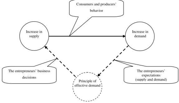
For Kaldor (1972), the growth process as a chain-reaction between increases in supply and increases in demand is understood when the principle of effective demand and increasing returns are taken into account. Of course, those considerations question the concept of “equilibrium economics” and come within the scope of the critiques made by Kaldor against this concept (Setterfield, 1998). I represent this growth process by the figure 1.

1.1. The weakness of current modellings

Kaldor did inspire the new theory of endogenous growth (Romer, 1986; Lucas, 1988; Aghion and Howitt, 1998) with his considerations about increasing returns (Palley, 1996; Hussein and Thirlwall, 2000), following Young (1928). But, in those models, the role of demand as well as the link between the division of labor, the increasing returns, the reduction of costs and the expansion of the markets have been disregarded (Rima, 2004). In fact, those models of the endogenous growth are still based on the neoclassical foundations of the growth theory. However, the research of steady states turns out to be a very good analytic tool (Palley, 1996). One must notice that the theory of endogenous growth, which aims at reconciling increasing returns and equilibrium economics, does not give us a satisfying explanation about the economic growth (Helpman, 2004). The endogenous growth remains “a speculative answer that needs to further investigated” (Acemoglu, 2009, p. 872). The lessons of those models seem to follow their hypotheses (Alcouffe and Kuhn, 2004). Moreover, by focusing on the sector of research and development- that generates innovations- those models rule out the role of entrepreneurs (Ebner, 2000).

The works of the post-Keynesians (like Davidson and Smolensky, 1964; Davidson, 2001, 2002; Arestis, 1996; Pasinetti, 2001, 2005) have shown the interest of the principle of the effective demand and its relevance on the long term. The Keynesian foundations for a new theory of the endogenous growth (Palley, 1996) underline the need to combine the mechanisms of endogenous growth (increasing returns) with the principle of effective demand and capital accumulation. For Palley (p. 114) “the conclusion is that Keynesian growth theory requires both the mechanisms of endogenous growth and that capital accumulation be governed by investment spending (rather than saving).”

At the same time, a lot of works dealt with the possible synthesis between Keynes' view and Schumpeter's (for example, Minsky, 1986; Goodwin, 1991, 1993; Davidson, 2002; Flacher and Villemeur, 2005; Bertocco, 2007). Let's quote Davidson (2002, p. 57), in particular: “If entrepreneurs have any important function in the real world, it is to make crucial decisions. Entrepreneurship, which is but one facet of human creativity, by its very nature, involves crucialities in a nonergodic setting. To restrict entrepreneurship to robot decision making through ergodic calculations in a stochastic world, as Lucas and Sargent2 _{do, ignores the role}

2

Lucas R., Sargent T. [1981], Rational Expectation and Econometric Practices. University of Minnesota Press, Minneapolis. Increase in supply Increase in demand Principle of effective demand The entrepreneurs’ expectations (supply and demand) The entrepreneurs’ business

decisions

Consumers and producers’ behavior

of the Schumpeterian entrepreneur - the creator of technological revolutions that bring about future changes that are often inconceivable even to the innovative entrepreneur.”

In order to show the relevance of Kaldor's conception, we must subscribe to the synthesis of the works inspired by Keynes and Schumpeter. Then, the Keynesian foundations seem to have two inadequacies. One concerns the explanation of the aggregate supply function (Davidson, 2001; Pasinetti, 2001). The other one concerns the way to take into account the innovation process (Bellais, 2004; Pianta and Tancioni, 2008). Those inadequacies lead us to go deeper into Keynes and Schumpeter's views of the role of the entrepreneur, since their originality and their interest seem to have been under estimated.

1.2. The behavior of the entrepreneur: Keynes and Schumpeter’s view

In his General Theory (1936),3 Keynes considers that entrepreneurs take decisions concerning the volume of output and employment according to an expectation4 of demand: the “effective demand”. This effective demand5 is given by the point of the intersection between the aggregate supply function Z =

ϕ

( )

L and the aggregate demand function D= f

( )

L ; at this point (the equilibrium of effective demand), the entrepreneurs’ expectation of profits will be maximized.

The employment determinants are mainly “the propensity to consume” and “the inducement to invest”. This latter is determined by the comparison between the marginal efficiency of capital, in other words the rate of return to capital which measures the expected yield from an investment, and the real interest rate. Thus the entrepreneur will only invest if the marginal efficiency of capital is higher than the real interest rate.

And so for Keynes (1936)6_{, short-term decisions must take account of long-term expectations}

regarding investment. Marginal efficiency of capital is thus a long-term expectation which depends on the state of confidence of the entrepreneurs and cannot be replaced by the current rate of return to capital.

With regard to the search for maximum profit (ex ante) undertaken by the entrepreneur, Keynes stresses the constraint represented by the “amount of employment to offer”.7 Keynes (1936, p. 141) also highlights the risk of long-term competition the entrepreneur takes: “The output from equipment produced to-day will have to compete, in the course of its life, with the output from equipment produced subsequently, perhaps at a lower labor cost, perhaps by an improved technique... Moreover, the entrepreneur's profit (in terms of money) from equipment, old or new, will be reduced, if all output comes to be produced more cheaply.”. The risk is all the greater in that the prospective yield is substantial and will bring other entrepreneurs onto the market.

“Workers will not seek a much greater money-wage when employment improves.” This conclusion by Keynes (1936, p. 253) has been widely confirmed by empirical research. In his investigation of 27 industrial sectors within the American economy between 1923 and 1950,

3

Chapter 5: “Expectation as determining Output and Employment” (p. 46).

4 _{For Keynes (1936, p. 46), the entrepreneur “has no choice but to be guided by these expectations, if he is to}

produce at all by processes which occupy time.”

5 _{“The value of D at the point of the aggregate demand function, where it is intersected by the aggregate supply}

function, will be called the effective demand.” (Keynes, 1936, p. 25).

6 _{“Nevertheless, we must not forget that in the case of durable goods, the producer's short-term expectations are}

based on the current long-term expectations of the investor…Thus the factor of current long-term expectations cannot be even approximately eliminated or replaced by realized results” (p. 51).

7

See for example Keynes (1936, p. 23-24): “The entrepreneur's profit thus defined is, as it should be, the quantity which he endeavors to maximize when he is deciding what amount of employment to offer.”

Salter (1960, 1966) noted the lack of correlation between labor productivity gains8 and employment growth. Other economists have also highlighted this fact in the United States in similar terms: there is no correlation between labor productivity and employment (Hansen and Wright, 1992).

For Schumpeter economic development has the characteristics of a process of evolution whose central figure is the entrepreneur (Nelson and Winter, 1982; Nelson, 2005, 2007; Hanusch and Pyka, 2007). As Nelson and Winter (1982) have emphasized, the process of evolution is one of continuing disequilibrium,9 given the decisions taken by entrepreneurs. This process is led by entrepreneurs who have identified opportunities for creating wealth via implementation of innovations.10

Schumpeter makes the distinction between “to produce more” and “to produce differently”.11 “To produce more” mainly covers additional production of existing products or production of new products; dissemination of product innovations is part of this. “To produce differently” mainly covers the transformation of production process with, for example, lower product costs; dissemination of process innovations is part of this. This distinction between “to produce more” and “to produce differently” is a most fundamental one, for the entrepreneur's decisions must take it into account. According to the types of investment, innovation can contribute either to create employments or to shed some of them (Goodwin, 1991; Lorenzi and Bourles, 1995; Pianta, 2006;12 _{Crespi and Pianta, 2008), which reflects the creative}

destruction at work.

For Schumpeter (1942, p. 97), the entrepreneur's aim is competitiveness, as the competitive goods market obliges producers to opt for the lowest total cost per unit of production: “Everyone agrees that private and socialist managements will introduce improvements if, with the new method of production, the total cost per unit of product is expected to be smaller than the prime cost per unit of product with the method actually in use”. In addition, profit is in essence “the result of carrying out new combinations” (Schumpeter, 1911, p. 136). In other words, the entrepreneur takes the production, investment and employment decisions so as to obtain the lowest total cost per unit of product, while drawing on available innovations; profit maximization becomes a more long-term goal.

And so, while Schumpeter stresses the aim of “short-term” competitiveness, Keynes foregrounds the aim of “long-term” competitiveness. In fact these two different points of view characterize two indissociable aspects of competitiveness.

Thus, Keynes and Schumpeter's views are complementary since they concern both the process of evolution resulting from entrepreneurs who take investment and innovation risks, and the process of entrepreneurs’ decisions about production, investment and employment.

8

The profit share in the income being a constant on the long term, the wage growth rate is equal to the labor productivity growth rate.

9 _{P. 276 :“Although these models have yielded some illuminating insights, they ignore essential aspects of}

Schumpeterian competition - the fact that there are winners and losers and that the process is one of continuing disequilibrium.”

10 _{Let’s quote Nelson (2007, p. 37): “economic growth needs to be understood as a process driven by the}

coevolution of physical and social technologies.”

11 _{Schumpeter, 1926 (second edition), p. 121. It should be remembered that for Schumpeter (1911, p. 65), “To}

produce means to combine materials and forces within own reach...To produce other things, on the same things by a different method, means to combine these materials and forces differently.”

12 _{Pianta (2006) has highlighted the stylized fact that product innovation helps create jobs while process}

innovation destroys them: “The evidence shows that it is essential to discriminate between product innovation (novel or imitation) that has a generally positive employment impact and process innovation (adoption or use of new technologies) usually with negative effects” (p. 590).

2. An entrepreneurial growth model based on the principle of effective

demand

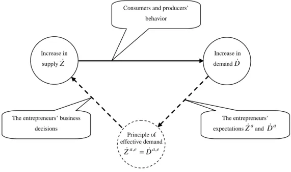
The new entrepreneurial growth model (figure 2) that we are presenting is based on the principle of effective demand for the short term period

[

t,t+dt

]

. The aggregate supply function, represented by Z&a =

ϕ

( )

L&a , is the additional (expected) volume of output resulting from the employment increase L& .a 13 _{The aggregate demand function, represented by}

( )

a a

L f

D& = & , is the additional proceeds which entrepreneurs expect to receive from employment increase L& . Let a D&a,e be the additional effective demand, the additional demand given by the point of intersection (for employment increase L& ) between the aggregate a,e supply function and the aggregate demand function.

Classically, the aggregate demand function that we are looking at is the same kind as Keynes’. However, the aggregate supply function is based on the complementary views of Keynes and Schumpeter. Entrepreneurs aim at creating new productive combinations by taking innovation opportunities. They try to “produce more” or “produce differently”.

Entrepreneurs implement capital and labor factors to meet an anticipated additional demand.14

They expect one part of the net investment15

to be a capacity investment associated with additional supply ( “to produce more”) while the other part is to be a process investment (“to produce differently”) associated with stagnant demand. The first type of investment will be called here “capacity investment”, with capital and labor coming together “to produce more” (with increasing returns). The second type will be called “process investment”, with capital taking the place of labor. While employment creation is associated with capacity investment,

13 _{a indicates the anticipated character of the variable (or ex ante).}

14 _{As Kaldor (1972, p. 1240), we assume that the markets are “instrument for transmitting impulses to economic}

change”.

15 _{The net investment is the (gross) investment minus the replacement investment.}

Increase in supplyZ& Increase in demandD& Principle of effective demand e a e a _D Z& , = & , The entrepreneurs’ expectationsZ&aand D&a The entrepreneurs’ business

decisions

Consumers and producers’ behavior

employment destruction is associated with process investment, thus reflecting the process of creative destruction at work.16

Investment and employment decisions are made according to the marginal efficiency of the capital that entrepreneurs consider for their investment project. Entrepreneurs aim at minimizing the total cost (per unit of additional supply) linked to the capacity investment they plan, taking into account the costs resulting from the workforce and the capacity investment. The minimization of the total cost can only take place under a constraint related to the amount of employment to be created. This constraint reflects the risk of being confronted to new competitors, this risk being all the more important since the marginal efficiency of the capital is substantial.

According to the principle of effective demand, the new equilibrium expected by entrepreneurs is the intersection of the aggregate supply function and the aggregate demand function. Now, I shall determine the aggregate supply function, then the aggregate demand function and the equilibrium of effective demand. At the initial time t , I assume that the supply Z , the demand D , and the production Y are in equilibrium (Z =D=Y).

2.1. The aggregate supply function

Taking into account the relationship between supply and investment, the effect of creative destruction on employment, and the necessary competitiveness of the new productive combinations, the aggregate supply function Z&a is defined.

The supply-investment relationship

Entrepreneurs anticipate an additional supply Z&a which they intend to meet by a net investment Ina, which comprises a capacity investment

(

0≤ ≤1

)

a a n a x I x and a process

investment

(

1−xa

)

I_na; xa is the share of the capacity investment engaged in the total volume of net investment. Entrepreneurs use the technology A characterized by a supply function17 of the type Z& = AK&, A being the marginal rate of productivity of the capital associated with the capacity investment;18 A will henceforth be termed “productivity of the capacity investment”. The productivity of the capacity investment is then assumed to remain constant. The additional supply will be met as follows:19

a n a a I Ax

Z& = with I_na =K&a 0≤xa ≤1 ⇒

Z I Ax Z Z a na a = & (1) a

x will be called anticipated “growth multiplier”, with any increase in x leading to faster a growth in supply.

The creative destruction

Entrepreneurs plan to create jobs according to the additional supply, supply-employment elasticity being variable:

L L e Z Z a ac c a = & eca >1 (2)

16 _{Thus, capital and labor inputs are in part substitutable and in part complementary with increasing returns to}

scale.

17 _{This function is taken, via differentiation in relation to time, from the form (Y=AK) proposed by Harrod}

(1939) and Domar (1947) but also by Nelson and Winter (1982) to represent Schumpeter's analysis.

18 _{In accordance with the Nelson-Phelps (1966) approach, it is acknowledged that human capital is not a}

production factor; thus the variable of the capital K will not include human capital.

where La_c is employment creation associated with capacity investment xaI_na. It is accepted that the jobs created are more productive, given the innovation brought by the investment and the increasing returns; whence an elasticity higher than 1. Thus the employment creation anticipated by the entrepreneur is:20

a n a a c a n a a c a c x I Y L I x Y L e A L = =ε with _a c a c e A = ε 0<εca < A (3)

The coefficient εca, called anticipated “employment creation coefficient”, is obviously variable, given the variable character of elasticity.21 _{In the same way the entrepreneurs plan to}

cut employment according the “supply deficit”A

(

1−xa

)

I_na, elasticity also being assumed as variable. Thus the employment destruction L anticipated by the entrepreneurs is: a_l

a n a a l a l x I Y L L =ε (1− ) ε_la ≥0 (4)

The coefficient ε_la, called anticipated “employment destruction coefficient”, is also variable. I assume now that there is a link between the choices of employment creation and employment destruction, and clarify it via two considerations. When the entrepreneurs choose highly creative combinations of jobs, the combinations chosen for capital-labor substitution destroy fewer jobs; this reflects confidence in additional supply in terms of the firm's products as a whole. Furthermore there are limits to the creation and destruction of employment, these limits depending on the technology used. These choices of productive combinations are reflected in the following relationships:

mx c a l a c ε ε ε + = cmx a c ε ε ≤ < 0 cmx a l ε ε < ≤ 0 εcmx < A (5)

where ε_cmx is the maximum coefficient of employment creation,22 a characteristic of technology A. This latter parameter reflects the organizational limit of the creation or destruction of employment, given the forms of organization set up by the entrepreneurs in the context of the use of technology A. Thus, the anticipated increase in employment is:

(

)

a n mx c a c a mx c a l a c a I Y L x L L L& = − = ε +ε −ε 0<ε_ca ≤ε_cmx ε_cmx < A (6)

The increase in employment depends on the values anticipated for the variables of the volume of net investment, of the growth multiplier and of the employment creation coefficient.

The competitive productive combination

In order to meet an additional anticipated supply a

Z& , in the context of a marginal efficiency of capital e , entrepreneurs can implement various productive combinations involving the _K growth multiplier xa, the employment creation coefficient ε_ca and the volume of investment

a n

I . They will then decide on the combination that fits with the aim of the lowest cost and the aim of expected profit. The appendix 1 shows that the conditions are the following:

20

At the beginning of the short-term period: Z=D=Y.

21 _{Keynes (1936, p. 286) clearly considers demand-employment elasticity as highly variable: “If, for example,}

the increased demand is largely directed towards products which have a high elasticity of employment, the aggregate increase in employment will be greater than if it is largely directed towards products which have a low elasticity of employment.”

cA e xa = K c e_K a c = ₋ 1

ε

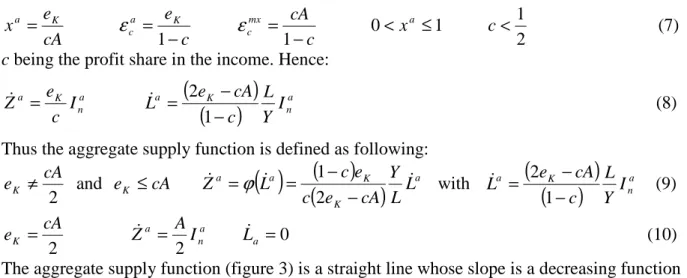
c cA mx c = ₋ 1 ε 0<xa ≤1 2 1 < c (7)

c being the profit share in the income. Hence:

a n K a I c e Z& =

(

)

(

)

na K a I Y L c cA e L − − = 1 2 & ₍₈₎

Thus the aggregate supply function is defined as following: 2 cA eK ≠ and eK ≤cA

( )

( )

(

K

)

a K a a L L Y cA e c e c L

Z& & &

− − = = 2 1

ϕ

with

(

)

(

)

na K a I Y L c cA e L − − = 1 2 & ₍₉₎ 2 cA eK = a n a I A Z 2 = & _{L&a =0 (10)}

The aggregate supply function (figure 3) is a straight line whose slope is a decreasing function of the marginal efficiency of capital.23

2.2. The aggregate demand function

The aggregate demand function is the additional volume that the community (producers and consumers) is expected to spend on consumption and to devote to investment, taking into account the anticipated increase employment. We suppose that the (anticipated) marginal propensity to consume is p_Ca_&. Hence:

a a a C a I Z p

D& = _& & + & 0< p_Ca_& <1 (11) The anticipated additional demand is a function of the anticipated marginal propensity to consume, of the aggregate supply function, and of the anticipated increase of the investment. Hence:

( )

₍

( )

₎

a a K K a C a a I L L Y cA e c e c p L f

D& & _& & + &

− − = = 2 1 (12)

23 _{The marginal efficiency of capital is less than cA (growth multiplier less than 1).} a D&

E

a I& e a Z& , a Z& Z&a a D&

0

a L& e a L& ,

The aggregate demand function (figure 3) is also a straight line that intersects the aggregate supply function. We assume that the relation between net investment and investment is simply: Ina =(1−δ)Iawhere δ is the replacement investment rate, a constant in time. Hence:

( )

₍

(

)

₎

) 1 ( 2 1

δ

− + − − = = a na K K a C a a I L L Y cA e c e c p L f

D& & _& & & (13)

2.3. The equilibrium of effective demand

In a general case, the equilibrium is determined by the intersection of the two functions (figure 3):

(

)

(

)

(

)

na K a C K e a I Y L e c p cA e c L& & & 1 (1 ) 1 2 ,

δ

− − − − = K _na a C a n e a e a I c e p I D Z = − − = = ) 1 )( 1 ( , ,

δ

& & & & (14)

The employment increase depends on the marginal propensity to consume, on the marginal efficiency of capital, and on the net investment increase. Here, we find a result that is consistent with Keynes’ General Theory and we recognize, in the latest equation, the expression of investment multiplier 1/

(

1− p_Ca_&

)

.

Thus, after having defined the marginal efficiency of capital e_K, the marginal propensity to consume p_Ca_& and the volume of investment I , entrepreneurs are able to determine the _na additional effective demand D_&a,e

, the employment increase L_{& , the growth multiplier} a,e a

x and the investment increase I&_na.

a n K e a e a I c e Z D& , = & , =

(

)

( )

na K e a I Y L c cA e L − − = 1 2 , & cA e xa = K na K a C a n I c e p I& =(1− _&)(1−δ) (15) The entrepreneur's choices can be readily interpreted: when he anticipates a rise in marginal efficiency, he reduces the volume of investment, while anticipating a higher growth multiplier (a higher proportion of capacity investment) and greater employment growth so as to keep on coping with the same additional effective demand.

It is important to note here that the growth rates for demand and employment which are anticipated for the short term are linked by a linear relationship independent of the marginal efficiency of capital, in other words, independent of the view entrepreneurs formulate for the long term: Y I A L L c c Z Z D D na e a e a e a 2 2 1 , , , + − = = & & & (16)

3. The stationary states of an economy

The growth process is made of a succession of increases of supply and demand, induced by a succession of equilibriums of the effective demand. I shall show that, in the long term, stationary states do exist and that these are steady states within which growth rates for output and employment are constant over time. To identify stationary states I make the classical assumption that the entrepreneur's anticipations have been fulfilled in reality, that the marginal propensity to consume is a constant over time,24

and that growth is balanced, notably in the sense of the work of Harrod (1939, 1948) and Domar (1947). On the long term, I

suppose that there is no correlation between the labor productivity growth rate and the employment growth rate.

3.1. The determination of stationary states

Anticipations and realities in the long term

The anticipated values of the fundamentals encounter reality: Y

Z D Z

D&a,e = &a,e = & = & = & L&a,e =L& n a

n I

I = xa = x n

a

n I

I& = & p_Ca_& = p_C&

K P q eK & & = = (17)

where P is the profit (equal to cY ) and q is the rate of return to capital.25 In the long term, for an additional output Y& , entrepreneurs decide to invest I_n and to increase employment by

L& and investment by I&n according to the following formulae:

26 n I c q Y& =

(

)

( )

In Y L c cA q L − − = 1 2 & cA q x= n

(

C

)

In c q p I& = 1− _& (1−δ) (18) In addition, the equality between supply and demand (and between the increases) implies the following formulae: C p s i Y E Y I − = = = = 1 p_C Y E Y I & & & & & − = = 1 (19) where i ,s, p are the (gross) investment rate, the (gross) saving rate_C and the average propensity to consume. We assume that the marginal propensity to consume is a constant equal to the mean propensity to consume. Hence:

= = C C p p_& constant ⇒ = = = =i =s = − p_C = Y E Y I Y E Y I 1 & & & & constant (20) Thus, the net investment rate and the net saving rate are constant on the long term.

Balanced growth in the Harrod and Domar sense

We assume that the output growth rate is equal to the capital growth rate (“warranted” growth rate); in other words the mean productivity of the capital is a constant for the long term:

= = ⇔ = ⇔ = K Y y K Y K Y K K Y Y K & & & & constant ⇒ = yKin = Y Y& constant (21) Given the relations (18):

= = = = K n in Axin c q i y Y Y& constant (22)

There are three consequences. The first consequence is the constancy of the growth multiplier: = = A y x K constant (23)

The second consequence is the constancy of the profit share in the income: K cy q= and K Y c Y c q & & & + = ⇒ c=constant (24)

The third consequence is the constancy of the (mean) return on capital z (equal to the rate of return to capital):

25

Here, the profit share in the income is not assumed constant.

= = = = cy q K Y c z _K constant (25)

Thus stationary states are characterized by the following equations: n Axi Y Y& ₌

(

x

)

i_n c cA L L 1 2 1− − = & y_K = Ax z =cAx 1 0<x≤ 2 1 <

c x=constant i_n =s_n =constant c=constant (26) We note that the relationship between output growth rate and employment growth rate is independent of the growth multiplier:

n i A L L c c Y Y 2 2 1 + − = & & (27) 3.2. The independence between wage growth and employment growth

In his General Theory Keynes stresses that wage growth and employment growth are independent of each other. In other words the labor market induces a standard wage increase that is imposed on all firms, whatever the employment growth rate. The wage growth rate must thus be independent of the employment growth rate. But given the invariability of the profit share in the income, the wage growth rate is equal to the rate of growth of labor productivity. Hence: n i A L L c c L L Y Y 2 1 2 1 +     − − = −

= & & &

&

ω

ω

0 1 2 1− _{− =} c c _⇔ 3 1 = c (28)

An immediate, striking consequence lies in the profit share in the income, which is invariably equal to 1/3. As a consequence, in the long term, the entrepreneur must introduce productive combinations27

in which the profit share in the income is equal to 1/3. 3.3. The existence of steady states

Fundamentals Equations

Output growth rate

n Axi K K Y Y = = & & 1 0<x≤ x=constant = = n n s i constant

Employment growth rate A

(

x

)

i_n

L L 2 1 2 − = &

Profit share in income

3 1 = c Capital productivity Ax K Y y_K = = Return on capital z Ax 3 =

A: productivity of the capacity investment x: growth multiplier n

i : net investment rate s_n: net saving rate

Table 1 - Expression of fundamentals in steady states

For the stationary states, the growth rates for output and employment remain constant over time. These stationary states thus have the property of steady states. Table 1 recapitulates the expression of the main fundamentals in steady states: they are expressed simply, according to the productivity of the capacity investment, the net investment rate (or saving rate) and the growth multiplier.

The productivity of the capacity investment and the investment rate are exogenous data. The former reflects the speed of technological progress allowed by the technologies used and the accompanying institutions. Thus it does not reflect the level of technological progress; a technologically backward economy can be characterized by productivity of the capacity investment higher than that of an advanced economy. The investment rate depends on the monetary conditions (not taken into account in the growth model).

4. Major insights

4.1. Significant results in the long term

The first significant result lies in the fundamental output-employment relationship as verified by steady states: n i A L L Y Y 2 + = & & with in =sn =constant (29)

The labor productivity growth rate is simply equal to the half-product of the net investment rate (or net saving rate) and the productivity of the capacity investment.

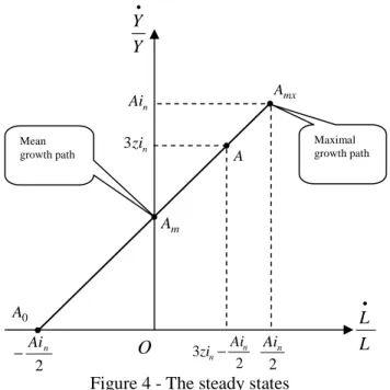
The set of stationary states is represented by A0Amx in Figure 4, the point A being excluded. 0 The slope of this segment is simply equal to the unit. The steady state associated with the return on capital z is the point A .A_mx represents the maximal growth path (for the long term); the output and employment growth rates are thus maximal, all the new productive combinations being engaged in increasing returns. A_m represents the mean growth path, the growth multiplier being equal to 0.5.

As a rule, the larger the share of investment committed to complementarity (production factors), the stronger the growth - and the return on capital. Put otherwise, the more

L L • Y Y •

Figure 4 - The steady states

mx A

O m A

2 n Ai Maximal growth path Mean growth path _A

2 3 n n Ai zi − 2 n Ai − n Ai n zi 3 0 A

entrepreneurs succeed in becoming involved in increasing returns, the higher the growth and the greater the return on capital.

The second significant result is to be found in the distribution of income: 2/3 for labor income, 1/3 for capital income. This means that whatever the technology A, the output growth rate, the employment growth rate, and the investment rate (or saving rate), the profit share in the income is a remarkable constant in the steady states.

The third significant result lies in the quest by entrepreneurs for maximum profit, an incentive for the entrepreneurs to push up the growth multiplier (or the capital productivity) that is to say to further fuel their investments with capacity investments:

      = Axi Y P Max _n 3 1

& with i_n =constant ⇒ x↑ (30)

If this strategy is born out by subsequent events (ex post), the entrepreneur will continue with it. The trajectory of the economy will then be a succession of steady states interrupted by periods of disequilibrium, with growth potential rising as a long-term trend.

4.2. From disequilibrium to steady states

The decisions taken by entrepreneurs instigate an authentic process of economic evolution. By its very nature this process is unstable, as reality continuously resists all prediction. Nonetheless, the process does possess stationary states in the long term when, classically, it is assumed that anticipations coincide with reality and growth is balanced. How then are we to interpret ongoing disequilibrium and the existence of a set of stationary states?

As a rule growth paths appear to be in disequilibrium, for example when competitiveness is not ensured because entrepreneurs have not attained the lowest unit production cost. One reason for these inappropriate choices classically results, as many economists have shown,28 from dependence on the technological trajectory. Taking competition into account, these entrepreneurs are then obliged in the long run to come up with adaptive anticipations: in other words, to adopt more competitive productive combinations or to fail (Nelson, 2005). The return to a competitive situation represented by steady states is thus obligatory for these entrepreneurs; however, in the periods that follow, other entrepreneurs are in danger of being non-competitive.

In continuous disequilibrium, the economic trajectories are thus going to endlessly get nearer to and further away from steady states, i.e. the segmentA₀A_mx. Thus the steady states are seen fairly much as "attractors" (Nelson, 2005; 29 Villemeur, 2008). Considering that the behavior of entrepreneurs, producers, consumers and markets is perfect, the attractor of steady states symbolizes an ideal chain-reaction.

When the net investment rate is constant, the attractor A0Amx has a double function on the long term: to represent the mean trajectory of the economy, and also to attract economic trajectories30 _{(for example annual trajectories). Thus, the means of the fundamentals (output}

28 _{See David (2000) for example.} 29

“In their analysis of certain economic phenomena, for example technological progress, many economists recognize that frequent or continuing shocks, generated internally or externally, may make it hazardous to assume that the system ever will get to an equilibrium; thus the fixed or moving equilibrium in the theory must be understood as an “attractor” rather than a characteristic of where the system is” (p. 66).

30

On the short term, economic growth higher than maximal growth path can be obtained, as can recession; these extreme cases can be interpreted as situations when the capacity utilization ratio is temporarily rising or falling

growth rate and employment growth rate) should belong to the attractor, while the latter should be identical to the linear regression established on the long term.

5. Comparison with empirical reality

5.1. Comparison with stylized facts

Via analysis of the fundamentals of the main economies of the 19th and 20th centuries, Kaldor (1961) has identified six stylized facts31 characterizing long-term economic growth. For Barro and Sala-i-Martin (1995)32 these facts are confirmed by the long-term data relative to today's developed countries:

• Fact 1: per capita output grows over time, and its growth rate does not tend to diminish • Fact 2: physical capital per worker grows over time

• Fact 3: the rate of return to capital is nearly constant33

• Fact 4: the ratio of physical capital to output is nearly constant

• Fact 5: the shares of labor and physical capital in national income are nearly constant • Fact 6: the growth rate of output per worker differs substantially across countries. Other stylized facts have been put forward by Barro and Sala-i-Martin (1995): • Fact 7: a certain stability of investment and saving rates

• Fact 8: a positive correlation between the output growth rate and the investment rate.34

It is easy to verify that the theoretical lessons of the growth model are potentially consistent with the stylized facts listed by Kaldor and Barro and Sala-i-Martin. Stylized fact 6 is compatible with the growth model if we assume that the productivity of the capacity investment and investment (or saving) rates differ from one country to another.

An income distribution of 1/3 for capital and 2/3 for labor has often been put forward, as numerous historical references testify. In Cobb-Douglas's first growth model (1928), the profit share in the income is a constant parameter evaluated at 30%. Worthy of mention is the evaluation for the United States in the years 1909-1949, with an average of 34%35 (Solow, 1957). An average share of 34% is also found for a set of economies around the year 1990 (Gollin, 2002).36

The income split between profit and wage has been well measured since the 1960s in respect of the main developed economies (European Commission, 2002). The largest developed economy -the United States- has always had a profit share37

of 30-33%, very close to the theoretical value of 33%.

while the growth multiplier still lies between 0 and 1. Thus the equivalent growth multiplier would be higher than 1 or negative.

31

Here I follow the presentation and the formulation provided by Barro and Sala-i-Martin (1995, p. 5).

32 _{Only fact n}o _{3 would seem debatable according to Barro and Sala-i-Martin (see below).}

33 _{Barro and Sala-i-Martin formulate this stylized fact as: “The rate of return to capital is approximately}

constant”. This does not appear to be systematically verified if real interest rates are considered as indicators. Like other economists, I have kept the initial Kaldor definition (return on capital).

34 _{Much research supports this point of view, including De Long and Summers (1991), Levine and Renelt}

(1992), Bernanke and Gürkaynak (2002), Acemoglu (2009).

35 _{Annually the share varies between 31% and 40%.} 36

This 34% average concerns a set of 41 countries, the profit share in the income varying from 20% to 35%.

5.2. Comparison with the United States economy (1960-2000)

The chosen period is 1960-2000, for which we possess precise annual data38 on growth of GDP and employment (in hours worked), and on the investment rate. The data used are presented in the appendix 2 (Table 3). We continue to consider the growth model with a profit share of 1/339.

Our knowledge of the average annual growth rates for GDP and employment, and of the investment rate, for the period 1960-2000, enables deduction of average values for the productivity of the investment capacity and growth multiplier (Table 2):

      − = L L Y Y i A n & & 2 Y Y Ai x n & 1 = (31)

United States economy 1960-2000

Fundamentals

Annual growth rate of GDP

Annual growth rate of employment Investment rate (net)

3.41% 1.64% 0.131 Growth model parameters

Productivity of the capacity investment ( A ) Growth multiplier (x)

0.27 0.96

Table 2 - The fundamentals of the United States economy (1960-2000) and the growth model

It turns out that the average fundamentals of the American economy are close to the maximal growth path, characterized by a growth multiplier of almost 1.

According to the theory, the steady states (attractor) must verify the fundamental output-employment relationship: 0177 . 0 + = L L Y Y& & in L L Y Y 135 . 0 + = & & (32) The fundamental output-employment relationship (by linear regression)

I shall verify the existence of such a correlation between, on the one hand, the annual GDP growth rates and on the other the annual employment growth rate (in hours worked) and the net investment rate. The correlation between output and employment is significant,40 as is that between output, employment and net investment:41

0188 . 0 94 . 0 + = L L Y Y& & n i L L Y Y 145 . 0 92 . 0 + = & & (33) (0.10) (0.0025) (0.11) (0.020)

38

The data sources are the World Bank (World Development Indicators-WDI) for the GDP growth rate and the gross investment rate, and the Groningen Growth and Development Centre (Total Economy Database, January 2007, http://www.ggdc.net) for the growth rate of the total number of hours worked. As the data bases do not provide net investment information, it has been presumed that the proportion of replacement investment is the classical 30%.

39 _{The mean profit share in income (1960-2000) is 31.1% (European Commission, 2002).}

40 _{The values in parentheses are the standard errors for the coefficients. The R2 is 0.68. The statistics of Student}

T are respectively 9.00 and 7.48.

41

The correlation appears significant given the standard errors (in parentheses) for the coefficients, and the statistics of Student T, respectively 8.61 and 7.34.

Annual GDP growth rates correlate well with the employment growth rates and with the net investment rate, the employment coefficient remaining very close to 1.42 Examination of the annual performances of the American economy for the period 1960-2000 confirm that employment growth rate and the investment rate correlate closely with GDP growth rate. It appears that relations (32) and (33) are very similar. Figure 5 shows the annual positions on the economic trajectory for the period 1960–2000, together with the fundamental output-employment relationships. These latter were obtained theoretically from average annual values over the period (relation 32), and empirically by linear regression (relation 33).

Figure 5 illustrates the unbalanced character of annual economic growth and the role played by the steady states. The trajectory of the fundamentals curls around steady states which then appear to play the part of an attractor; the long-term average values of the fundamentals are consistent with those of the steady states. This reflects the fact that the instabilities are, in a way, channeled around the long-term relationship characterizing the stationary states of the growth model.

Productivity of the capacity investment and return on capital

From the coefficient relating to long-term investment (1960-2000) the result is a productivity of the capacity investment of 0.29, which tallies with the value of 0.27 obtained from long-term average values (Table 2). Working from these evaluations, the theory enables prediction of a return on capital of 8.7% to 9.3%: x A z 3 = with x=0.963 A=0.27 or 0.29 ⇒ z =8.7% or 9.3% (34)

42 _{Interestingly, Bernanke and Parkinson (1991), in their study of changes in production and employment in ten}

industries for the periods 1924-1939 and 1955-1988, found in the linear regressions an average employment coefficient of 1.07 and 0.96 respectively. In 72% of cases the coefficients for the different sectors fall between 0.8 and 1.3. They are obtained from quarterly observations for each of the ten industries.

Figure 5 - The United States economy (1960-2000) and the steady states

GDP growth rate (in %)

Employment growth rate (in %)

Linear regression Attractor (steady states) -2 -1 1 2 3 4 5 6 7 8 -3 -2 -1 0 1 2 3 4 5

This theoretical prediction appears satisfactory, the return on capital being measured at around 9-10% for this period.43 Thus the theoretical evaluation of return on capital seems consistent with the productivity of the capacity investment measured over the long term.

Conclusion

Kaldor’s view of a chain-reaction and the complementary points of view of Keynes and Schumpeter have been represented by a new entrepreneurial growth model based on the principle of effective demand. It has been shown that, in the long term, this process admits steady states with unexpected properties.

In the steady states, output and employment growth rates verify the following fundamental output-employment relationship: n i A L L Y Y 2 + = & & avec in =sn =constant

in which A is the productivity of the capacity investment, and i the net investment rate (or net n saving rate). It has been demonstrated that the steady states are theoretically characterized by a profit share in the income equal to 1/3. The trajectory of the growth paths curls around the steady states which then appear to play the part of an attractor for the long term.

The theoretical lessons to be drawn from the model prove consistent with the stylized facts provided by Kaldor and Barro and Sala-i-Martin, and with the stylized fact of a constant value - around 1/3 - for the profit share in the income. For the period 1960-2000 the American economy is characterized by a fundamental output-employment relationship that matches the growth model.

Eventually, those results reinforce the view of a growth process modeled as a chain-reaction between increases in supply and increases in demand.

43 _{Several evaluations support this estimate. Romer (1996, p. 93) puts it at 10% as a long-term trend. The OECD}

(1996, p. 184) puts it at 9.1% for the period 1974-1993. And in the course of the 1990s it moved up from 9% to 11% (European Commission, 2002).

REFERENCES

ACEMOGLU D. [2009], Introduction to Modern Economic Growth, Princeton University Press, Princeton and Oxford. AGHION P., HOWITT P. [1998], Endogenous Growth Theory, MIT Press, Cambridge.

ALCOUFFE A., KUHN T. [2004], « Schumpeterian endogenous growth theory and evolutionary economics », Journal of

Evolutionary Economics, 14, p. 223-236.

ARESTIS P. [1996], « Post-Keynesian economics: towards coherence », Cambridge Journal of Economics, 20, p. 111-135. BARRO R.J., SALA-I-MARTIN X. [1995], Economic Growth, McGraw-Hill, Inc., First MIT Press edition, 1999,

Cambridge.

BELLAIS R. [2004], « Post Keynesian theory, technology policy, and long-term growth », Journal of Post Keynesian

Economics, spring, vol. 26, n°3, p. 419-440.

BERNANKE B.S., GURKAYNAK R.S. [2002], “Is Growth Exogenous? Taking Mankiw, Romer, and Weil Seriously”,

NBER Macroeconomics Annual 2001, Vol. 16, MIT Press, p. 11-56.

BERNANKE B.S., PARKINSON M.L. [1991], « Procyclical Labor Productivity and Competing Theories of the Business Cycle: Some Evidence from Interwar U.S. Manufacturing Industries », Journal of Political Economy 99, June, p. 439-459.

BERTOCCO G. [2007], « The characteristics of a monetary economy: a Keynes-Schumpeter approach », Cambridge Journal

of Economics, 31, p.101-122.

COBB C.W., DOUGLAS P.H. [1928], « A Theory of Production », American Economic Review 18, March, p. 139-165. CRESPI F., PIANTA M. [2008], « Diversity in innovation and productivity in Europe », Journal of Evolutionary Economics,

volume 18 (3), August, p. 529-545.

DAVID P.A. [2000], « Path Dependence, its critics and the quest for « historical economics », Economic History, February. DAVIDSON P. [2001], « The principle of effective demand: another view », Journal of Post Keynesian Economics, spring,

vol. 23, n°3, p. 391-409.

DAVIDSON P. [2002], Financial Markets, Money and the Real World, Edward Elgar, Cheltenham, UK. DAVIDSON P., SMOLENSKY E. [1964], Aggregate Supply and Demand Analysis, Harper and Row, New York.

DE LONG J.B., SUMMERS L.H. [1991], « Equipment Investment and Economic Growth », Quarterly Journal of

Economics, 106, 2 (May), p. 445-502.

DOMAR F.D. [1947], « Expansion and Employment », American Economic Review, 37, March, p. 34-55.

EBNER A. [2000], « Schumpeterian Theory and the Sources of Economic Development: Endogenous, Evolutionary or Entrepreneurial? », International Schumpeter Society Conference on « Change Development and Transformation: Transdisciplinary Perspectives on the Innovation Process », Manchester, 28 June - 1 July.

EUROPEAN COMMISSION [2002], European Economy, 2001 Review, n° 73, Brussels.

FLACHER D., VILLEMEUR A. [2005], « Gouvernance d’entreprises et croissance économique : un modèle de croissance à répartition endogène », Deuxième colloque « L’économie politique de la gouvernance », Centre d’Etudes Monétaires et Financières, Dijon, 2 et 3 décembre.

GOLLIN D. [2002], « Getting Income Shares Right », Journal of Political Economy, vol. 110, n°2, p. 458-474.

GOODWIN R.M. [1991], « Schumpeter, Keynes and the theory of economic evolution », Journal of Evolutionary

Economics, 1, p. 29-47.

GOODWIN R.M. [1993], “Schumpeter and Keynes”, in Markets and Institutions in Economic Development, Biasco S., Roncaglia A., and Salvati M. (eds.), Macmillan, London.

HANSEN G., WRIGHT R. [1992], « The Labor Market in Real Business Cycle Theory », Federal Reserve Bank of

Minneapolis, Quarterly Review, 16, spring, p. 2-12.

HANUSCH H., PYKA A. [2007], « Principles of Neo-Schumpeterian Economics », Cambridge Journal of Economics, 31, p. 275-289.

HARROD R.F. [1939], « An Essay in Dynamic Theory », Economic Journal, 49, March, p. 14-33. HARROD R.F. [1948], Towards a Dynamic Economics, Macmillan, London.

HELPMAN E. [2004], The Mystery of Economic Growth, The Belknap Press of Harvard University Press, Cambridge. HUSSEIN K., THIRLWALL A.P. [2000], « The AK model of « new » growth theory in the Harrod-Domar growth equation:

investment and growth revisited », Journal of Post Keynesian Economics, spring, vol. 22, n°3, p. 427-435. KALDOR N. [1956], « Alternatives Theories of Distribution », Review of Economic Studies, vol. 23, p. 94-100.

KALDOR N. [1961], « Capital Accumulation and Economic Growth », in The Theory of Capital, F.A. Lutz, D.C. Hague, eds., Macmillan, London.

KALDOR N. [1972], « The Irrelevance of Equilibrium Economics », The Economic Journal, Vol. 82, No. 328, p. 1237-1255, December: p. 1240, 1246.

KEYNES J.M. [1936], The General Theory of Employment, Interest and Money, Macmillan, London (edition 1964). LEVINE R., RENELT D. [1992], « A sensitivity Analysis of Cross-Country Growth Regressions », American Economic

Review, 82, 4, September, p. 942-963.

LORENZI J.-H., BOURLES J. [1995], Le choc du progrès technique, Economica, Paris.

MINSKY H. [1986], “Money and Crisis in Schumpeter and Keynes”, in The Economic Law of Motion of Modern Society, Wagener H., Drukker J. (eds.), Cambridge University Press, Cambridge.

NELSON R.R. [2005], Technology, Institutions and Economic Growth, Harvard University Press, Cambridge.

NELSON R.R. [2007], “Understanding economic growth as the central task of economic analysis”, in Perspectives on

Innovation, Malerba F., Brusoni S., Cambridge University Press, Cambridge.

NELSON R.R., PHELPS E.S. [1966], « Investment in Humans, Technological Diffusion and Economic Growth », American

Economic Review 61, p. 69-75.

NELSON R.R., WINTER S.G. [1982], An Evolutionary Theory of Economic Change, Belknap Press of Harvard University, Cambridge.

OCDE [1996], Etudes économiques de l’OCDE, Etats-Unis, 1996, OCDE, Paris.

PALLEY T.I. [1996], « Growth Theory in a Keynesian mode: some Keynesian foundations for new endogenous growth theory », Journal of Post Keynesian Economics, fall, vol. 19, n°1, p. 113-135.

PASINETTI L.L. [2001], « The principle of effective demand and its relevance in the long run », Journal of Post Keynesian

Economics, spring, vol. 23, n°3, p. 383-390.

PASINETTI L.L. [2005], « The Cambridge School of Keynesian Economics », Cambridge Journal of Economics, 29, p. 837-848.

PIANTA M. [2006], « Innovation and Employment », in The Oxford Handbook of Innovation, Fagerberg J., Mowery D.,C. Nelson R.R., Oxford University Press, p. 568-598.

PIANTA M., TANCIONI M. [2008], « Innovations, wages and profits », Journal of Post Keynesian Economics, fall, vol. 31, n°1, p. 101-123.

RIMA I.H. [2004], « Increasing returns, new growth theory, and the classicalism », Journal of Post Keynesian Economics, fall, vol. 27, n°1, p. 171-184.

ROMER D. [1996], Advanced Macroeconomics, McGraw-Hill, Inc., New York.

ROMER P.M. [1986], « Increasing Returns and Long-Run Growth », Journal of Political Economy, October, 94: 5, p. 1002-1037.

SALTER W.E.G. [1960, 1966], Productivity and Technical Change, Cambridge University Press, Cambridge.

SCHUMPETER J.A. [1911] Die Theorie der wirtschaftlichen Entwicklung, Duncker & Humblot, Berlin, The Theory of

Economic Development, 1934, Harvard University Press, Cambridge, Massachusetts [first edition 1911]. Second edition,

1926, French Translation, Théorie de l’Evolution économique, 1999, Dalloz, Paris.

SCHUMPETER J.A. [1942], Capitalism, Socialism and Democracy, Harper and Brothers (1942, 1947, 1950) First Harper Colophon edition (1975).

SETTERFIELD M. [1998], « History versus equilibrium: Nicolas Kaldor on historical time and economic theory »,

Cambridge Journal of Economics, 22, p. 521-537.

SOLOW R.M. [1957], « Technical Change and the Aggregate Production Function », Review of Economics and Statistics 39, p. 312-320.

VILLEMEUR A. [2008], « Economic Growth, an evolutionary process characterised by an attractor », 12th International

Schumpeter Society Conference, July 2-5, Rio de Janeiro.

YOUNG A. [1928], « Increasing Returns and Economic Progress », The Economic Journal, Vol. 38, No. 152, December, p. 527-542.

APPENDIX 1- The competitive productive combination

The lower cost

In the context of capacity investment, the entrepreneur chooses the productive combination which minimizes the anticipated total cost per unit of additional supply. The anticipated total cost (Costa) includes the cost of the increase in employment - the wage

ω

being assumed constant - and the cost of the capacity investment, given the required marginal efficiency of the capitale . The anticipated total cost per unit of additional supply is: _K

(

)

K a c a n a a n a K a c a n a a e A A c I Ax I x e L I Ax Cost ₌

ω

+ ₌ 1−

_ε

₊ 1 xa ≠0 (A1.1)

c being the profit share in the income, so that

ω

L=

( )

1−cY. The entrepreneur's aim is then to determine the optimal productive combination

(

ε_ca,e_K

)

. The constraint indicates that the anticipated cost of the creation of employment, per unit of capacity investment, is inversely proportional to the marginal efficiency of capital: