ECONOMICAL ANALYSIS OF PRODUCT STANDARDIZATION
Vincent GIARD
Professor at the IAE in Paris • Panthéon - Sorbonne University ([email protected]) Abstract: The standardization of partially substitutable components destined to meet a set of needs is studied. The monocriterion approach to standardization proposed in the last century is highlighted by taking into account several criteria and an economic valorization through model-ing by linear programmmodel-ing. The notion of diversity is analyzed in this perspective and some cost
problems of this method are discussed. Copyright © 2000 IFAC.
Keywords: standardization, product design, mass production, linear programming.
Calibration was the main standardization effort in the era of craftsmanship. It dealt with the establishment of measures (monetary, weight, length, etc.) in order to determine the exchange of goods and services on compa-rable bases and to progressively build the related sci-ences. One has to wait for the industrial revolution, which came about through the evolution of knowledge, before the use of standardized processes allowed production of substitute products, enabling the production of ever more complex finished products manufactured from identical components made on machines, which are also becoming increasingly sophisticated. This product standardization is compatible with a systematic production of “custom” component most often used in a single product. The design rationalization of a range of homogeneous and partially interchangeable products, designed to meet var-ious needs, presented here as the modern definition of product standardization, is rapidly felt. We begin with the relationships between diversity and standardization before proposing a lead to optimize this standardization.
1. DIVERSITY AND STANDARDIZATION
After an overview of standardization fundamentals, the diversity concept will be examined in detail
1.1. Standardization fundamentals
Standardization efforts are undertaken in all industrial-ized countries in the first half of the nineteenth century. In France, it seems that modeling of this rationalization dates back to the mid 1800s with the work of Renard on French navy ropes: increasing ship sophistication, with custom-designed rigging, and colonial expansion led to a rapidly unmanageable proliferation of rope stocks. The idea is quite simple. In this problem, the main
character-istic of a rope is the maximum tensile strength Y that a
rope of diameter X can withstand before rupturing. A test
on ropes of various diameters helped establish Figure 1. Then, subdivide the axis of ordinates into a definite
num-ber of disjoint intervals and associate, to any yk tension
request, the diameter associated with the upper limit of
the interval that contains yk (i.e., in the example on Figure
1, a rope of diameter x2, for a limit traction before rupture
between y1 and y2).
This approach to the problem can limit the number of item-types to produce and manage, but the number of intervals and their definition remain to be solved. To do so, empirical work proposed solutions (and gave birth namely to the “Renard series” still used in the industry). Before proposing an economic modeling of this problem under a multicriteria generalization approach, it could be useful to put the problem in a larger perspective of diver-sity and its cost, in an economic context that further aims at interesting the client through custom production of goods and services.
1.2. Diversity Analysis
The global perception of finished products by the con-sumer or the potential client is not discussed here. That perception is conditioned by numerous factors; several depend on the mix-media selected in marketing and are of no concern to us. We only consider the visible produc-tion diversity on components of a finished product satis-fying needs of an identical nature, the presence of one of these components being mandatory. Doing so, the
sup-Y X y3 x2 y2 y1 y4 Diameter Maximum tensile str ength befor e rupturing
Fig. 1. Analysis of traction limit before rope rupture, by Renard
plementary diversity obtained by adding optional
com-ponents is not analyzed1.
Three types of custom production must be differenti-ated (See Anderson and Pine, 1997). Some product char-acteristics can be customized by the client for a perfect
suitability with his tastes or needs (customizable
prod-ucts). For example, the owner of a stereo sound system
can set up certain characteristics of his tuner so the sound of his stereo system matches his preferences, the driver of certain makes of automobiles can adjust the height and inclination of the steering wheel, or the PC user can modify the parameters of his work environment.
Other products (customizing products) are self-adapting,
meaning they automatically adjust to the context of their utilization, which is namely to ensure the function for which they are designed. This product category can be illustrated by the electric shaver with floating heads or by washing machines using fuzzy logic to determine the best wash cycle (this is progress compared to washing machines customized with a few dozen washing pro-grams, between which the user often has trouble decid-ing). Finally, some products are customized by the manufacturer (and, in some cases, by the salesperson).
Several non-exclusive solutions can describe this
cus-tomization.
• The best known approach is the use of an appropriate
combination of modules, each module being selected from a limited number of interchangeable modules. This solution, largely used in the automotive industry, not only implies a standardized production process (to minimize settings and tool changes) and a total substi-tutability of modules from a same family during assembly, but also the design of standardized assembly supports called product platform (Meyer and Lehner, 1998) to limit the “system risks” of malfunction, assured of sufficient lastingness and robust, i.e. accept-ing a large spectrum of constraints (electrical, mechan-ical, etc.).
• The use of adjustable components with reversible
set-tings leads to immediate and cost-efficient customiza-tion of a component by different means (switch, software…) to activate a set of functions selected from a predetermined list; this decision could be reversed. This technique of often selected in the design of elec-tronic or electric components.
• The use of adjustable components with irreversible
adjustments corresponds to an immediate and cost-effi-cient adaptation of a component to the needs either by additional machining operations, or by a chemical treatment, both irreversible. Such products are found in the cutting trade, eyewear, custom bicycle manufactur-ing, or replacement doors and windows. Deferred dif-ferentiation often arises from this logic.
There are thus several ways to reach diversity of a fin-ished product that avoid referring to systematic and costly customization. Two standpoints determine their economical analysis.
• A component is not a priori designed to be solely used
in one finished product due to design, manufacturing and distribution synergies. The question of product design rationalization of a company must therefore be treated from a standpoint of technologically similar product families rather than from each individual prod-uct, taking into account that the industrial classification analysis of complex products with a same basic com-ponent is normally found in several different aggregate products (commonality). The question of product design rationalization deals with meeting a set of basic functional needs through a range of physically inter-changeable components, each component with a lim-ited spectrum for each of the functional needs selected. This approach to standardization makes it one compo-nent of company flexibility, complementing resources (equipment, personnel, procedures).
• This component variety must be detectable by the cli-ent and he must consider it an added value. There are numerous examples of diversity detectable by the cli-ent but of no added value for him. For example, Nissan decided to rationalize its supplies in 1993; it had more than 300 ashtrays for its vehicles (stated in Anderson & Pine, p. 95). Product internal diversity not detectable by the client is even worse (screw-products are a clas-sical example of this type of diversity). Not only is it of no added value for the client, but it often generates additional costs (due to additional logistics problems, increased tooling diversity, etc.).
More often than not, a technical analysis of the classifi-cation of production and supply item-types will show a significant portion of components with identical or very similar characteristics. This mushrooming effect has sev-eral and well known explanations: misunderstanding of the impact of mushrooming item-types on production and product support service, the NIH syndrome (Not Invented Here), arbitrary design decisions, misleading argument about the “proper weight, etc.”, failure of the information system – all leading to the faster creation of a new item-type rather than looking up an existing one. It is clear that the economic approach to standardization that will be developed hereunder is of interest only if causes for mushrooming are not detected and progres-sively eliminated.
Searching to optimize standardization supposes on one
hand that functional needs are adequately assessed and
translated into technical specifications, which is facili-tated by the QFD approach (Quality Function
Deploy-ment2), and on the other hand that a coherent and
relevant reflection is carried out on all solutions consid-ered adequate. It is obvious that the optimum solution of a poorly stated problem is not of a great interest (it even could reflect discredit on the method and not on its mis-use). Determination of the solution portfolio to examine is based on a study eliminating a priori none of the cus-tom modes described above. What already exists (inter-nal manufacturing or supply) must of course be part of the alternatives studied and the new products planned must take into account the constraints of the existing production system or the one undergoing
transforma-tion3. Optimizing this standardization not only normally
results in a decrease of production costs, but also in an 1. This type of diversity generates additional costs when the
prod-uct is assembled on an assembly line due to the work variability caused by the assembly of optional components on some work-stations, creating specific line balancing and scheduling prob-lems (See Danjou, Giard and Le Roy, 2000). It may be economically interesting to systematically offer a popular option and if demand focuses on a few alternative options, it is then pos-sible to relate to the method described here. Inversely, one can question the economic interest of least popular options.
2. The Quality Function Deployment is a value chain optimization technique, from expression of needs to product support service. It originated in Japan and has been used for over 20 years by major companies, especially with the first step of the approach to switch from functional needs to technical specifications. An over-view of these techniques is found in Revelle, Moran and Cox, 1997.
increase flexibility, the company could then react more rapidly and easily to the conjunctural and structural
transformations of demand4.
2. TOWARD OPTIMIZING STANDARDIZATION
Once the general modeling of the problem stated by linear programming, we will examine a few methodolog-ical problems stated by this economic rationalization, whether we call on the proposed optimization approach or not.
2.1. Baseline model
For simple and non-expensive products (for example screw-products or the above-mentioned Nissan ash-trays), a sophisticated analysis is generally not manda-tory as long as the reduction in the number of components for a function becomes self-evident from a classification simplification standpoint as well as for pro-duction and supply processes.
In other cases, the Renard approach is used to rational-ize the range of relatively simple products, generally characterized by a unique quantitative criterion. Pareto analyses on need distribution based on this quantitative criterion (See, for example Anderson & Pine, chap. V, 1997) establish empirical approaches to determine a range of products, but the action is based on intuition and barely takes into account the economic standpoint. Prod-uct complexity also ensures that the technical analysis cannot have only one criterion. Formulation of this prob-lem by linear programming using integers brings
rele-vant response elements to these concerns5; the matrix
generators approach tested can easily implement them6.
The model will be presented with an example on engines. From a technical standpoint, we have n possible
variants of a product7, whether these variants are
pres-ently produced or only under study. These different
vari-ants will be identified with the subscript j. Moreover, we
presume the demand analysis identified m segments,
identified with the subscript i and characterized by a
demand dι. From an existing situation, we must normally
have , i.e. the variety of the commercial offer is
lower than the variety of the demand.
The problem at hand is first related to an eventual decrease in the number of variants (with no economic vision of the problem). A first technical analysis must be performed to characterize the various engines. Selected criteria relate to technical characteristics that are more or less well perceived by demand (power, pollution, consumption…) and to characteristics of no interest for the client but essential in managing interfaces (weight, overall dimensions, engine mounting method on the chassis…). This technical analysis is performed on a table similar to Table 1, with a literal in each table cell to indicate the precise positioning of each engine.
A second analysis is to be carried out on technical characteristics of requested engines (Table 2). For each previously determined criterion, an interval of admissi-ble values (minimum power, for example) is then defined based on the type of characteristic or a list of acceptable occurrences is determined if the characteristic is qualita-tive (such as mounting mode, for example). A difficulty encountered is determining the “appropriate need” aimed at pleasing, as mentioned above.
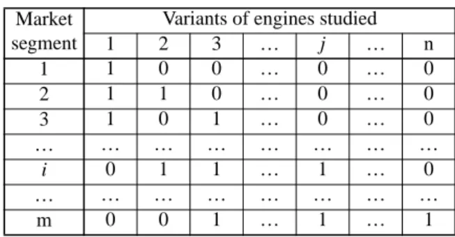
Comparing Tables 1 and 2 establishes Table 3, in
which coefficients aij take the value 1 if demand in
seg-ment i can be met by engine j, or 0 if it cannot be met
(the numerical illustration being fully arbitrary).
It seems realistic to impose that the entire demand seg-ment be satisfied by a same variant. Consequently, we
define the binary variable xij, which will have the value 1
if demand of segment i is met totally by an engine j, and
0 if it is not. It is of course useless to create a variable xij
3. This category of concern is taken into account in DFA (Design For Assembly) literature; refer to Nof, Wilhelm and Warnecke, 1997, chap. III, and to Redford and Chal, 1994.
4. Company flexibility (See Tarondeau, 1993 & 1997, Cohendet and Llerenna, 1989, and Reix, 1997) is classically seen through mobilized resources (equipment, tooling, personnel and proce-dures); product-related flexibility is generally highlighted but, however, economic instruments for its improvement have not been studied much to our knowledge, and not in the perspective treated here.
5. In an previous research document (Giard, 1990), we presented briefly a similar model in a more restrictive perspective. In a recent publication (Giard, 1998), we proposed a system approach to production process modeling through mathematical program-ming indicating the mutual connections between various models found in the literature on operational research and explaining the complex model creation mechanisms using a set of base compo-nents. Formally, the problem here combines a transposition of a client assignment model to production centers (Giard, 1998, p. 46) and the recognition of non-linear costs with fixed costs that vary by brackets (Giard, 1998, p. 97), except that the total pro-duction of an item-type here is the sum of propro-ductions requested by various segments.
6. This MGs approach is described in Murphy, Stohr and Asthana, 1992, Rosenthal, 1996, Jacquet-Lagrèze, 1997 and Giard, 1998. The technical and economic viability of this method is proven in numerous achievements (for example, two important industrial applications of these methods were carried out at the IAE in Paris within the scope of research contracts; they are described in Giard, Triomphe and André, 1997, and in Giard and Triomphe, 1996).
7. Renault’s Cléon plant, for example, manufactures more than 400 possible engine variants.
Table 1: Technical characteristics of engines under study Engines under study Characteristics 1 2 … p 1 2 j n
Table 2: Technical characteristics of requested engines Requested engines Characteristics Demand 1 2 … p 1 d1 2 d2 i di m dm
Table 3: Possibilities of satisfying the demand with the offer
Market segment
Variants of engines studied
1 2 3 … j … n 1 1 0 0 … 0 … 0 2 1 1 0 … 0 … 0 3 1 0 1 … 0 … 0 … … … … i 0 1 1 … 1 … 0 … … … … m 0 0 1 … 1 … 1 n m≤
if the corresponding parameter aij is null8. Moreover, if we decide that this demand can be met by several
vari-ants, then variable xij can have any value between 0 and
1. To force the demand of segment i to be met, we must
establish the constraint of Relation 1 (which leads, for binary variables, to a non null value).
, for i = 1,…., m (meeting the demand) Relation 1
Under these conditions, production yj of item-type j is
then the sum of productions carried out for each segment
(demand di), this production could be null. This
con-straint is defined by Relation 2:
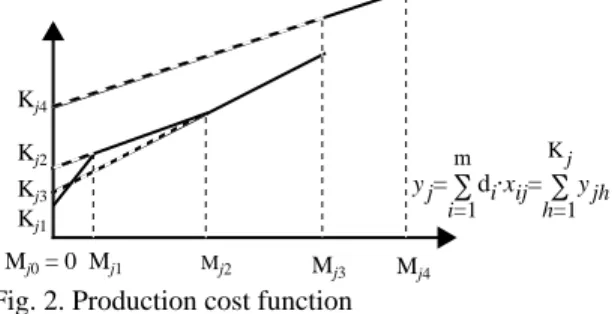
, for j = 1… n (production of item-type j) Relation 2 To establish the annual production cost, we must intro-duce explicit hypotheses on the item-type costs function form. First, we will assume the cost functions are inde-pendent. This restrictive hypothesis will be removed later on. We will also assume variation in annual fixed costs per bracket, and that for each bracket the variable unit cost may vary but remains constant over disjoint value intervals; these very general hypotheses lead to a cost function of the type described in Figure 2.
This cost function is neither concave (which would imply that the mean production cost never increases
when yj increases) nor convex (which would imply that
the mean production cost never decreases when yj
increases) and that in the selected example it takes into account the phenomena of scale diseconomies occurring at the saturation limit. This non-linear cost function can easily be taken into account in the objective function of a
linear program by introducing as many dummy yjk
pro-ductions as there are Kj value intervals (comprised
between Mj,k-1 and Mj,k, the upper threshold only is
included in the interval, with Mj0 = 0) for which the
vari-able cost cjk is constant, and are all null except for the
one encompassing production yj in its value interval and
that is, of course, equal to this production (yj = yjh). From the example in Figure 2, the objective function becomes,
for the section related to production cost yj:
Min z, with z = (cj1yj1 + Kj1zj1) + (cj2yj2 + Kj2zj2) +
(cj3yj3 + Kj3zj3) + (cj4yj4 + Kj4zj4) +…
with the following list of constraints9, added to those of
Relations 1 and 2:
The first constraint ( ) activates at
most one of the fixed costs (Kjkzjk), the one for which zk
= 1, providing that if this item-type is not produced, all
zjk are null. The following constraints force a 0 value on
yjk productions of intervals that are not selected for the
two limits are nul when zjk = 0, forcing the
correspond-ing production xk to be null, and vice versa10.
Generalizing the reasoning to all variants leads to the Relation 3 objective function and to the constraints described by Relations 4 and 5:
Min
z
, withz
= Relation 3, for j = 1… n Relation 4
, for k = 1… Kj and j = 1… n,
with Mj0 = 0 Relation 5
This formulation must be adapted to take into account positive or negative synergy effects related to simulta-neous production of two or more engines on a produc-tion site. To do so, relevant and easy modeling tools have
to be implemented11. Let us examine a few examples.
• Let us assume that manufacturing more than κ variants
translates into an increase of annual fixed costs; we
then have to create the binary variable, add to the
objective function the term , and add Relation 6
constraints to force to take the value 1 if at least κ
variants are produced (the objective function is
designed to bring to equal 0).
Relation 6 Of course, this relation can easily be adapted to a sub-set of engines or to several engine subassemblies. In the latter, the subsets can be disjoint, which will occur when technically specialized tool sets are used in the production of different engine sets. The same engine set can also be found in several constraints of this type. This allows defining the fixed costs as a step function of the number of item-types produced and not as a function of the total quantity produced.
• Let us assume, on the contrary, that manufacturing
more than κ variants means a decrease of annual
fixes costs; we then have to create the binary
vari-able, subtract the term from the objective
func-tion and add Relafunc-tion 7 to constraints to force to
only take the value 1 if at least κ variants are produced
(the objective function is designed to bring to equal
1). 8. This special feature, easy to take into account in the problem
description by a GM (see, for example, Giard, 1998, and Jaquet-Lagreze, 1997) helps in significantly limiting the size of the problem. This convention makes Relation 1 useless in the form
9. As variables are not negative, the first double constraint is in
real-ity reduced to x1≤ M1y1; the selected formulation has the sole
advantage of allowing rationale generalization.
aijx ij j 1= n ∑ =1 xij j 1= n
∑
=1 yj di⋅xij i 1= m∑
= Kj1 Kj2 Kj3 Mj1 Mj2 Mj3 Kj4 Mj4 Mj0 = 0 yj di⋅xij i 1= m ∑ yjh h 1= Kj ∑ = =Fig. 2. Production cost function
10.If the cost function is concave (non-decreasing total cost func-tion), then the “straight section” of double unequations is useless. 11.See Giard, 1998, chapter III.
zj1+zj2+zj3+zj4≤1 0 y≤ j1<Mj1zj1 Mj1zj2≤yj2<Mj2zj2 Mj2zj3≤yj3<Mj3zj3 Mj3zj4≤yj4<Mj4zj4 zj1+zj2+zj3+zj4≤1 ckyjk+Kjkzjk ( ) k 1= Kj
∑
j 1= n∑
zjk k 1= Kj∑
≤1 Mjk 1– zjk≤yjk<Mjkzjk Γ+ γ+ γ+Γ+ γ+ γ+ zjk k 1= Kj∑
j 1= n∑
<κ nγ+ + Γ -γ -γ-Γ -γ -γ-Relation 7 Here again, this approach can easily be adapted to a subset of variants or to several variant subsets. Among others, nothing precludes positive or negative synergy effects to occur simultaneously for different variant subsets or not, as a generalization of the previous com-ments.
• We can assume finally that certain fixed costs vary per bracket with relation to produced quantities over a set of item-types, notwithstanding the possibility offered for each item-type to include in its cost function its own variation of fixed costs per bracket. In this case, the Ω engine subset being affected by variations of
fixed costs, we simply have to adapt the formulation as follows:
- create variable ω corresponding to the total
produc-tion of the Ω engine subset, which leads to Relation
8:
Relation 8 - add to the objective function the impact of variations
in fixed costs Kωk, following the same method used
for item-type
;
- then adapt Relations 2, 4 and 5, which leads to Rela-tions 9 to 11
Relation 9
Relation 10 , for k = 1… Kω, with
Relation 11 2.2. Method problems created by using this
optimiza-tion approach
The relevance of this modeling depends both on its the use to describe alternate scenarios and on the costs used in the economic function.
First, we are working at a detail level too coarse to pre-tend it accurately represents the processes used, the effective demand on the production system, with its sea-sonal and random fluctuations, or the robustness of the production system when faced with problems. This com-ment can be made for most help tools on strategic deci-sions: the important aspect is the relevance of the order of magnitude of collected data in volume or in value. This brings us back to valorization problems.
The most important problems we may meet here relate to time or, more specifically, correctly defining the inter-dependence through time of decisions made within the cost accounting system.
In the rare case where the studies alternatives relate to new production from new equipment, it is easy to see the use of a dynamic version of the model proposed, as the decision to meet a demand segment by a given engine is
taken for all periods12; other hypotheses can be used, but
seem more difficult to justify. The separation between fixed costs and variable costs helps isolate start-up
investments (and thus avoid the problem of determining the depreciation) from direct fixed costs (especially per-sonnel) that could vary per bracket with relation to quan-tities produced and variable direct costs (materials, etc.). As this information used in the economic function is
dated13, we would have to call upon actualization to
cor-rectly weight the monetary flows generated at different periods. Classic problems are encountered when this approach is applied to compare investment alternatives and, more specifically, to determine the determination of the interest rate used in VAN calculus and the problem of comparing solutions having different useful lives.
When the problem relates to a set of item-types that at least partially exists, when it is the object of external supply or an internal production in a production system which could eventually be only marginally modified, several methodology problems arise.
• Certain key components of a certain complexity are designed to be used in several finished products, some of which do not yet exist; the term “main sub-assem-bly” projects is used in the automotive industry. The transfer price of such components creates challenging
methodological projects14. A decision on
standardiza-tion that quesstandardiza-tions the economic hypotheses used to launch such components must rely on a cost function that guarantees decision coherence in time and between strategic and tactical decisions (See Giard, 1988 and 1992).
• Within this framework and more generally, the deci-sion to stop production of a item-type (or of a group of item-types) can lead to support an “item withdrawal cost”. This impact can easily be taken into account by
the objective function15.
• Existing standard costs are only relevant on a certain range of quantities produced or supplied; before apply-ing the method, thorough investigations are needed to reconstitute the cost function and, for supply, carry out a prior consultation with suppliers on the basis of vol-ume scenarios that could substantially deviate from the current solution.
• The standardization problem can occur within a multi-level bill of materials. Decisions taken at a detailed level then are based on hypotheses of direct demand and demand originating from other item-types (using MRP type mechanisms) that are themselves the object zjk k 1= Kj
∑
j 1= n∑
>κγ -ω yj j⊆Ω∑
di⋅xij i 1= m∑
j⊆Ω∑
= = Kωkzωk k 1= Kω∑
ω ωk k 1= Kω∑
≤ zωk k 1= Kω∑
≤1 Mωk 1– zωk≤ωk<Mωkzωk Mωk=012.Which can be translated by maintaining Relation 1 and the
fol-lowing adaptation of Relation 2 which becomes: ,
Relations 3 and 5 being modified by the inclusion of the period index, Relation 3 integrating actualization coefficients. 13.With an appropriate time sub-division, this helps take in to
account possible learning effects on recurring costs, with values that can be considered reasonably stable over each time interval. . 14.For a more complete presentation of problems related to eco-nomic management of products over their life cycle, refer to Gautier and Giard, 2000.
15.Using notations of Relation 4, for a cost of , simply add the
term in the objective function. Knowing that
if item-type j is produced, the cost will not be
sup-ported in this case alone. Generalization of a set of
item-types is immediate , with .
yjt dit⋅xij i 1= m ∑ = Φ 1 zjk k 1= Kj ∑ – Φ zjk k 1= Kj ∑ =1 Φ Ψ ψ 1 t– { }Φ zjk k 1= Kj ∑ j∈Ψ ∑ –ψ< t
of a standardization optimization. An independent analysis of these different problems cause the problem of elementary component standardization to depend on hypothetical aggregate component demands and cause the problem of aggregate component standardization to depend on hypothetical costs of elementary compo-nents. Convergence toward a set of coherent solutions can empirically be assured through a certain number of iterations, but this model could also be adapted to take
into account the Bill Of Materials16, which could lead
to a model of undue size.
• The creation of new components induces management costs related to increased diversity that are difficult to evaluate. In economic calculations made at the design stage, certain companies such as Intel or Renault apply different cost rates to new components and to reused existing components. This incentive to reduce diversity is astute but must be used with great caution within a complete reconsideration required when applying the approach suggested in this paper.
3. BIBLIOGRAPHY
Anderson D. M. , Pine II J. (1997). Agile Product Development for Mass Customization : How to Develop and Deliver Products for Mass Customization, Niche Markets, JIT, Build-to-Order and Flexible Manufacturing, McGraw-Hill, New-York.
Baldwin C. Y., Clark K. B. (1997). Managing in an age of modularity , Harvard Business Review, vol. 75 sept -oct 1997, p. 84-93.
Brooke A., Kendrick D. & Meeraus A. (1988). GAMS : A User’s Guide, Scientific Press, Redwood City.
Cohendet P. , Lléréna P. (1989). Flexibilité, information, déci-sion, Economica, Paris.
Danjou F., Giard V., Le Roy É. (2000). Analyse de la robustesse des ordonnancements/réordonnancements sur ligne de production et d’assemblage dans l’industrie automobile, to be published in Revue Française de Gestion Industrielle, vol. 19, n°1, Paris.
Giard V. (1990). Analyse économique de la diversité en produc-tion, working paper G 90/2, 1990, URA CNRS 1257, IAE de Lyon.
Giard V., Pellegrin C. (1992). Fondements de l’évaluation économique dans les modèles économiques de gestion , Revue Française de Gestion, n°88, p. 18-31.
Giard V., Triomphe C. (1996). SIAD visant à définir les services offerts au personnel d’un centre de production et s’appuyant sur la programmation mathématique, working paper 1996.03, IAE de Paris (see http ://panoramix.univ-paris1.fr/ GREGOR/96-03.pdf).
Giard V. (1998). Processus productif et programmation linéaire, Economica, Paris.
Giard V., Triomphe C., André R. (2000a). Organist : un Système Interactif d’Aide à la Définition du niveau de trai-tement du courrier des bureaux de poste et des tournées d’acheminement à un centre de tri, to be published in Cahiers du Génie Industriel, vol. 1, n° 1.
Gautier F., Giard V. (2000b). Evaluation économique des choix de conception d’un produit nouveau : l’impact sur les
systèmes productifs, accepted in the proceedings of the AFC 2000 Conference, 18-20 may 2000.
Jacquet-Lagrèze E. (1997). Programmation Linéaire – Modéli-sation et mise en œuvre informatique, Economica. Meyer M. H., Lehner A. P. (1998). The power of product
plat-forms - building value and cost leadership, The Free Press, New-York.
Murphy F., Stohr E., Asthana A. (1992). Representation schemes for linear programming models , Management Science, vol. 38, n° 7, pp.964-991.
Nof S. Y., Wilhelm W. E., Warnecke H.-J. (1997). Industrial assembly, Chapman & Hall, London.
Redford A., Chal J. (1994). Design for assembly : principles and practice, Mac-Graw Hill, New-York.
Reix R. (1997). Flexibilité , Encyclopédie de gestion, (Y. Simon & P. Joffre Ed.), 2° edition, Economica, Paris.
Revelle J. B., Moran J. W. , Cox C. (1997) The QFD Handbook, Wiley,.
Rosenthal R. E. (1996). Algebraic Modeling Languages for optimization , Encyclopedia of Operations Research and Management Science, S. I. Gass & C. M. Hyarris ed., Kluwer Academic Publishers, Boston..
Smith P. G., Reinertsen D. G. (1998). Developing Products in Half the Time : new rules, new tools, second édition, Wiley, New-York.
Tarondeau J.-C. (1993). Stratégie industrielle, Vuibert, Paris. Tarondeau J.-C. (1999). La flexibilité dans les entreprises, PUF,
Paris.
Williams H. P. (1993). Model Building in Mathematical Programming, 3e edition, Wiley, New-York.
16.Simply replace Relation 2 ( ), which defines
pro-duction , as being equal to the sum of demands related to it
by binary variables , with the following Relation:
, where item-type h is related to item-type j due to the production of 1 item-type h unit requires unit of item-type j. (This item-type h is related to final demands through Relation 2).
yj di⋅xij i 1= m ∑ = yj di xij yj di⋅xij i 1= m ∑ ahj⋅ ⋅yhxhj h 1= m ∑ + = ahj