Insurance Contracts with Imprecise Probabilities
and Adverse Selection
∗
Meglena Jeleva
LEN-C3E, Université de Nantes, EUREQua
106-112, Bld de l’Hôpital
75647 Paris Cedex 13
France
E-mail: [email protected]
Bertrand Villeneuve
†IDEI Université de Toulouse 1
Place Anatole France
31042 Toulouse cedex
France
E-mail: [email protected].
April 11, 2003
Abstract
This article deals with optimal insurance contracts in the framework of imprecise probabilities and adverse selection. Agents differ not only in the objective risk they face but also in the perception of risk. In monopoly, a range of configurations that VNM preferences preclude appears: a pooling contract may be optimal, incomplete coverage may be offered to high risks, low risks may be better covered.
Keywords: Imprecise Probabilities; Insurance Markets; Adverse Selec-tion.
JEL: D81, D82, G22
∗Useful suggestions by Emmanuelle Auriol, Bernard Bensaïd, Michèle Cohen, Isaac Meilijson
and the anonymous referee are acknowledged.
1
Introduction
Following Rothschild and Stiglitz [7] and Stiglitz [10], asymmetric information in insurance markets is generally understood as a situation in which consumers are better informed than insurers. However, the general perception in insurance com-panies is quite different: statistical discrimination and risk assessment have made considerable progress, whereas individuals often have limited and biased experience. One could even estimate that adverse selection is eradicated in certain markets (see Chiappori and Salanié [1] for evidence). If we go further and assume that insurers are better informed on risk, then the issue would rather be to inform people correctly on their risks rather than design sophisticated menus. Along these lines, Villeneuve [11] proposes an analysis of the better informed insurer in which the question of information transmission is explored.
Both the adverse selection hypothesis and its reverse contain some truth: insurers know risk better, at least as far as the classifications they use are concerned, whereas consumers know something personal and unobservable that is also relevant to risk. This paper is a modest attempt to reconcile these two points of view. On the one hand, we assume that customers, though “knowing their types”, may not correctly process all the information attached to this knowledge. On the other hand, insurers are able to define risk classes and measure which “types” are pooled in a given statistical class and what risk they bear; however they are assumed to be unable to assign a type to a given customer.
How can insurers know these stable traits of their clientele? Experimentation, whether optimized or involuntary, combined with revealed preference arguments, justifies that statistical parameters of interest be inferred from actual choices. This knowledge can be capitalized to improve contract offers to new groups of consumers. We shall assume that we are at the final stage of this learning process that we do not model.
Several arguments can justify our assumption concerning risk perception by con-sumers. Consumers very often have limited experience, imprecise sources of infor-mation, and consequently their beliefs remain durably inaccurate. A young driver may know that his accident probability is high without being able to quantify it precisely, and this may produce biases in his choice of insurance coverage.
More-over, even if agents have perfect knowledge of their true probability distribution, a disparity between beliefs and objective probabilities is still rationalizable. A now classical representation is the rank dependent expected utility (Quiggin [6], Yaari [12]).
To summarize, we are in a situation where asymmetric information has two sides. Insurers do not distinguish ex ante high risk consumers from low risk consumers, whereas the policyholders do not necessarily behave as they should if they were perfectly informed or just expected utility maximizers. To simplify matters and avoid difficulties with equilibrium concepts that arise in the competitive case, we consider here a monopolistic insurer.
The results of the paper are as follows. A difference between beliefs and prob-abilities in an insurance model with adverse selection, in addition to making the model closer to reality, explains a wider range of configurations. A striking fact is that, though the single-crossing property remains satisfied everywhere, the optimal offer of the monopolistic insurer can be a pooling contract over a continuum of para-meters. The reason for this is that the marginal values for a better coverage across types may be ranked by types and by insurers in opposite ways: the most costly type may be the one with the least willingness to pay for coverage. This “disagree-ment” cannot always be resolved with differentiated offers. The distinction between beliefs and probabilities introduces the possibility of the low risk (in terms of ob-jective probability) being more covered than the high risk. We obtain an important difference with Stiglitz’ model [10]; our findings stress the fact that it is crucial for insurers, when they decide the contracts they offer, to take into account the possible differences between agents’ beliefs and probabilities. After a theorem giving the general properties of our model, we characterize the particularities of the various possible configurations, and we show exactly how the equilibrium moves when the distribution of types is changed.
Section 2 briefly recalls several models of decision making under risk and ambi-guity justifying the existence of a difference between beliefs and “true”probabilities. In section 3, we define and examine the first-best optimum when insurance appli-cants’ beliefs differ from the true probabilities, but insurers can perfectly categorize applicants according to the true risk they present. Section 4 sets the problem of the monopolistic insurer confronted with a heterogenous population in terms of beliefs
and probabilities when the insurer cannot distinguish applicants according to their true risks. We establish a theorem that sets the general necessary properties of the optimal menu in this second-best context. In section 5, we consider different pos-sible configurations of the parameters and give a complete characterization of the optimal solutions. Proofs are relegated to the Appendix.
2
Beliefs and objective probabilities
In this section, we briefly present several distinct reasons why insurers’ and policy-holders’ risk assessments may differ. Though meanings differ, most of these cases are formally identical, which enables us to include them in the same mathematical framework.
A consumer with initial wealth W0 incurs a loss d with probability p which
represents the “true” (or objective) probability as estimated by the insurer. An insurance contract C = (W1, W2) is fully characterized by the individual’s wealth
in all states of nature: W2 if loss occurs, and W1 otherwise. C0 represents the null
“contract” (W0, W0−d), i.e. no insurance. We denote by V the function representing
consumer’s preferences on contracts.
When consumers know their objective loss probability, a disparity between V and expected utility (EU) is rationalizable by the rank dependent expected utility model (RDEU) proposed by Quiggin [6] and Yaari [12].1 Preferences depend on the
one hand on a utility function (reflecting perception of wealth) and on the other hand on a probability transformation function (reflecting perception of loss distribution). The whole characterizes attitude towards risk. In our simple context, the utility can be expressed:
VRDEU(C) = ½
(1− ϕ(1 − p))u(W2) + ϕ(1− p)u(W1) if W2 ≤ W1
(1− ϕ(p))u(W1) + ϕ(p)u(W2) if W1 ≤ W2 (1)
where ϕ is an increasing probability transformation with ϕ(0) = 0 and ϕ(1) = 1. A consumer with concave u is risk averse if ϕ(x) < x, ∀x ∈]0, 1[, i.e. if he underestimates the probabilities of higher wealth and overestimates that of lower wealth. Risk seeking corresponds to ϕ(x) > x.
When consumers lack precise information (ambiguity), several preference repre-sentations are possible.
In the general case where information doesn’t take a particular form, it is pos-sible, under certain axioms, to represent preferences using the subjective expected utility (SEU) model of Savage [8]. We get:
VSEU(C) = qu(W2) + (1− q)u(W1), ∀ W1, W2 (2)
where q is the subjective loss probability.
Experimental violations of EU axioms (in particular the independence axiom) inspired the development of new, more general models of decision making under uncertainty. The Choquet expected utility (CEU) proposed by Schmeidler [9] is one of the most widely accepted models in this class. Consumers’ preferences depend on the one hand on a utility function and, on the other hand, on an increasing set function, a capacity, defined on events. This representation separates attitude towards uncertainty and attitude towards wealth. Denote by ω2 the event {loss
occurs} and by ω1 the event {no loss}; CEU is representable by
VCEU(C) = ½
(1− ν(ω1))u(W2) + ν(ω1)u(W1) if W2 ≤ W1
(1− ν(ω2))u(W1) + ν(ω2)u(W2) if W1 ≤ W2
(3)
where ν is a capacity with ν(∅) = 0 and ν(Ω) = 1 (Ω is the set of events). In a two-state context, an individual with concave utility function is “ambiguity averse” if ν(ω1) + ν(ω2) < 1, i.e. if he underestimates the likelihood of an event associated
with high wealth compared to event associated with low wealth.
If available information is just a probability interval (imprecise probabilities), we can refer to Jaffray [2]. The model, which generalizes EU, can be used whenever the information is that the true probability distribution belongs to a given set satisfying certain properties. Preferences are represented by a utility function and a pessimism-optimism index reflecting attitude towards ambiguity. With this Jaffray imprecise probabilities (JIP) model, if the consumer knows that p ∈ [q0, q00], the preference representation function can be expressed:
VJIP(C) = ½ ((1− α)q0+ αq00)u(W 2) + (1− (1 − α)q0 − αq00)u(W1) if W2 ≤ W1 (1− αq0− (1 − α)q00)u(W 1) + (αq0 + (1− α)q00)u(W2) if W1 ≤ W2 (4) where α is the Hurwicz pessimism-optimism index. By definition, α is such that the decision maker is indifferent between: (i) obtaining at least the lowest wealth
and at most the highest wealth with no information about the probabilities and (ii) obtaining either the lowest wealth with probability α or the highest wealth with probability 1 − α. If α = 1, the individual is a pure pessimist who assigns all the chances to the worst wealth.2
In the following, we assume the so-called indemnity principle: we rule out con-tracts for which the policyholder’s wealth is higher when he has an accident. This precaution prevents ex post moral hazard or incentives for destruction. In addition, “negative” insurance contracts (i.e. such that W1 − W2 > d) are forbidden to
sim-plify the analysis of corner solutions. We denote by C the set of contracts verifying these restrictions.
Under these assumptions, as we have W2 ≤ W1, all the previous models boil
down to one, where the consumer’s preferences can be represented by the following functional:
V (C) = qu(W2) + (1− q)u(W1) (5)
with q being a synthetic belief having a specific meaning in each of the models. To simplify the terminology, a consumer will be called pessimist if q > p, optimist if p > q, and neutral if p = q.
3
Insurance contracts
This section is devoted to the characterization of optimal contracts offered by a fully informed monopolistic insurer to a policyholder whose beliefs and objective probabilities differ. Note that a policyholder’s beliefs are assumed here not to be influenced by the insurer’s offer. Indeed, in case of ambiguity, the policyholder is assumed not to be aware of the insurer’s informational advantage, or at least unable to update his beliefs after observation of the offer he is made, and more generally to learn. If the policyholder knows the objective probability, but has RDEU preferences, the question of learning is obviously irrelevant.
The contract (W1, W2)offered by a risk neutral monopolistic insurer maximizes
its expected profit under the participation constraint of the consumer:
max
(W1,W2)∈C
(1− p) (W − W1) + p (W − d − W2) (6)
subject to
(1− q) u(W1) + q u(W2)≥ (1 − q) u(W ) + q u(W − d). (7)
Introducing λ as the Lagrange multiplier for the constraint, the first-order conditions can be expressed:
−(1 − p) + λ(1 − q)u0(W1) = 0, (8)
−p + λqu0(W2) = 0,
λ [(1− q) u(W1) + q u(W2)− (1 − q) u(W ) − q u(W − d)] = 0.
Stiglitz [10] proved that, with symmetric information regarding risk, a monopolistic insurer maximizing its profit offers a full coverage contract such that the policyholder is indifferent between purchasing the policy and having no insurance. The optimum is different here. Define
θ≡ µ q 1− q ¶ Áµ p 1− p ¶ . (9)
The optimal contract C∗ = (W∗
1, W2∗) verifying W2 ≤ W1 is such that:
u0(W1∗) u0(W∗ 2) = µ q 1− q ¶ Áµ p 1− p ¶ if θ < 1 W∗ 1 = W2∗ otherwise (10)
with the binding participation constraint:
(1− q) u(W1∗) + q u(W2∗) = (1− q) u(W ) + q u(W − d). (11) An insurance contract is efficient in our framework if it maximizes profit for a given utility level (or if it maximizes utility for a given profit level), that is whenever the marginal rate of substitution of the consumer equals the marginal rate of substitu-tion of the insurer, except if this rule leads to a contradicsubstitu-tion with the indemnity principle. In short, a contract is said to be efficient if and only if
u0(W1)
u0(W2) = min{θ, 1}. (12)
In the following, I(θ) represents the set of efficient contracts (or equivalently, of contracts offering efficient coverage).
The contract offered by a monopolistic insurer having complete information about the consumer’s loss probability and belief is therefore the contract in I(θ)
which is equivalent, for the consumer, to no insurance. If θ < 1 (p > q), the policy-holder is optimistic, the efficient contract line is below the full insurance line, which corresponds to partial coverage. If θ ≥ 1 (p ≤ q) then full insurance is efficient, as in Stiglitz [10].
Figure 1 shows the optimal contracts for two possible values of θ. Constant profit lines are parallel to π = 0, the indifference curves passing through C0 for the two
values are given.
INSERT FIGURE 1 HERE
4
Optimal menu under adverse selection:
Gen-eral properties
Under the adverse selection hypothesis, consumers are assumed to be identical, except for the probability of having an accident: two risk classes coexist in the population, denoted by H and L. Their beliefs are respectively qH and qL with
qH > qL, and the true probabilities of loss are pH and pL; θH and θL are the ratios
of the perceived odds of loss to the actual odds as defined above. H denotes the type with the highest belief which is not necessarily the type with the highest true probability.3 This choice simplifies considerably the exposition because preferences
only (not objective probabilities) matter for choice and self-selection. Probabilities and beliefs are not necessarily positively correlated, but even if they are, a low risk (in terms of probability) could still be more pessimistic than the high risk.
The insurer knows true probabilities and beliefs in the population, as well as the type proportions denoted by λH and λL (λH+ λL = 1). We denote by CH and CL
the contracts that would be proposed to H and L, respectively, in the absence of adverse selection (they are the profit maximizing efficient contracts). With qH > qL,
as we assume, this allocation cannot be implemented with adverse selection.
The Revelation Principle being applicable, the problem of the monopolist is to propose a pair of contracts, CLand CH,that are incentive compatible and preferred
(weakly) to no insurance. Obviously, neither CL nor CH need to be different from
C0,nor do CLand CH need to be different from each other. The second-best optimal
3In case of equality, the problem is to find the optimal pooling contract and the distinctions we
contracts of a monopolistic insurer are solutions of the following program: max CL,CH∈C λLπL(CL) + λH πH(CH) (13) such that CL ºL CH CL ºL C0 CH ºH CL CH ºH C0 (14)
where ºi, with i = L, H, represents the preferences of type i on contracts; πi gives
the per capita profit made by the monopolist if type i selects the specified contract. The problem is similar to Stiglitz [10] or Landsberger and Meilijson [4],[5] hence-forth LM). However the methodologies that they adopt (which significantly differ) are not suited here because individually efficient contracts depend on type. We recall the most important features of Stiglitz’ [10] solution.
Proposition 1 (Stiglitz) In case of pure risk:
1. High risk consumers get full insurance.
2. Low risk consumers are indifferent between their contract and no insurance.
3. High risk consumers are indifferent between their contract and the low risk consumers’ one.
4. The two types never buy the same contract.
5. There is a number strictly between 0 and 1 such that if λH is higher, then the
offer degenerates to the symmetric information insurance contract of high risk CH, and low risk remains uninsured.
All these five points require reconsideration in our model. Concerning what LM calls the structure of indifference, we have:
Lemma 1 The second-best optimal pair of contracts offered by a monopolistic in-surer is unique and:
2. Type H consumers are indifferent between their contract and the type L con-sumers’ contract.
Predictions are weaker than in Stiglitz [10]. The lemma is “tight” in that predic-tions of Stiglitz that we exclude are in effect violated with well-chosen parameters. For example, type H may have a binding participation constraint (in this case, no insurance at all is the optimal offer); moreover, type L consumers may not exhibit a strict preference for their contract, which justifies pooling contracts. Another ma-jor difference is that it is not necessarily true that one type at least gets efficient insurance. Section 5 provides conditions for all these cases.
Remark If type L consumers receive insurance, then type H consumers obtain an informational rent, or more precisely, their utility is higher than it would be if they were the only type in the market.
This result is a direct consequence of the preceding lemma. Indeed, every time type L obtains nontrivial coverage, type H consumers’ participation constraint is not binding and thus their utility is higher than with CH.
Thanks to Lemma 1, we can reduce the number of unknowns in the insurer’s program from four (two per contract) to one, since once CL has been chosen among
contracts that are equivalent to C0 from type L’s viewpoint (choice is in a
one-dimensional set), CH is uniquely determined as the profit maximizing contract that
is equivalent to CL for H.
The choice of the parameter is arbitrary. To keep smooth objectives, we proceed in the following way. Let W be the certainty equivalent for H of C0. Let W be
the certainty equivalent for type H of CL. We have W ≤ W . To each t ∈ [0, 1],
we associate W (t) = (1 − t) W + t W . For each level of constant wealth W (t), we define CL(t) as the unique contract (W1(t), W2(t)) which is equivalent to W (t) for
H and equivalent to no-insurance for L: ½
(1− qL) u(W1(t)) + qLu(W2(t)) = (1− qL) u(W0) + qLu(W0− d)
(1− qH) u(W1(t)) + qHu(W2(t)) = u(W (t))
(15)
Given CL(t), CH(t) is defined as the most profitable incentive compatible contract
that the insurer can offer to type H :
CH(t) = arg max (W1,W2)∈C
subject to ½
(1− qL) u(W1(t)) + qLu(W2(t)) ≥ (1− qL) u(W1) + qLu(W2)
(1− qH) u(W1) + qHu(W2) ≥ (1 − qH) u(W1(t)) + qHu(W2(t)) (17)
The menus M (t) = {CH(t), CL(t)} , t ∈ [0, 1], all satisfy the properties of the lemma.
Menus are continuously parameterized, and CL(t)offers to type L a coverage strictly
increasing in t. See Figure 2.
INSERT FIGURE 2 HERE
For a given menu M (t), we can define profits πL(t) and πH(t). Our
parameteri-zation is such that πL(·) is strictly increasing (CL(t)gets closer to the optimal CL as
t increases) while πH(·) is strictly decreasing (CH(t) gets farther from the optimal
CH as t increases). The objective of the monopoly can be expressed as the choice
of t∗(λL):
t∗(λL) = arg max
t∈[0,1]λLπL(t) + (1− λL)πH(t) (18)
This program represents the classical monopoly trade-off between minimizing infor-mational rents given to H and maximizing profits realized on type L.
The theorem is the basis of the comparative statics we provide in the following section:
Theorem 1 At the optimum, the monopolistic insurer offers M (t∗(λL)), where λL
is the proportion of type L consumers, and
1. t∗(·) is a continuous function.
2. There are ξ0 and ξ1 (with 0 < ξ0 < 1 and ξ0 < ξ1) such that:
(a) if λL ≤ ξ0, then t∗(λL) = 0 : H receives CH (no informational rent) and
L receives no insurance,
(b) if λL ≥ ξ1, then t∗(λL) = 1 : L receives CL and H receives the maximal
informational rent.
(c) if θL≤ 1, then ξ1 = 1 and if θL> 1, then ξ1 < 1.
3. Between extremes (ξ0 < λL< ξ1), t∗(·) is strictly increasing: as the proportion
Though Stiglitz’ [10] remains silent on this question, it is impossible in his model that types be pooled at CL. The reason is as follows: taking t slightly smaller than
1 has second-order effects on πL(t) (we just move away from the optimum for type
L) whereas it has first-order effects on πH(t) (CH(1) is not optimal for type H).
Consequently, whatever the respective proportions of types, t yields a higher profit than 1.
In our model, if type L is sufficiently pessimistic (θL> 1), the optimal contract
for type L, CL, is only a constrained optimum (since type L would prefer
over-insurance), meaning that the effect of t on πL(t) at t = 1 is of the first order.
This implies that types may be pooled at CL if there are sufficiently many type L
policyholders.
The threshold ξ0is always between 0 and 1. Indeed, moving t from 0 to a slightly positive value has first order effects on the profitability of both types, negative on type H and positive on type L. If λL is small, then it is more profitable to choose
t = 0, in other words to offer insurance to type H only.
5
Equilibrium configurations
The equilibrium configuration depends on the proportions of types in the population (λH and λL) and on the parameters θL and θH determining efficient insurance
cov-erage. Theorem 1 shows that the proportions directly affect the optimal trade-off between offering the most profitable contract to L while not conceding too large informational rent to H. This is true for almost any monopoly models with asym-metric information, including Stiglitz’.
The novelty of our results originate in the type specific parameters θH and θL.
The gap between probabilities and beliefs, i.e. between θH or θL on the one hand
and 1 on the other, determines whether or not at least one type is fully covered in equilibrium, and the difference between θH and θL determines whether or not types
are separated in equilibrium.
A general remark is necessary at this point. The equilibrium allocation must be interpreted carefully when the higher belief individuals (who are willing to pay more for complete coverage) obtain a higher coverage than the low belief individuals. Indeed, individuals with the higher belief may be, objectively, the low risk consumers
(pH < pL): thus, in this model, it is not always true that the best coverage and the
informational rent are obtained by the high objective risk type; risk perceptions, and consequently, behaviors, are the critical factors.
5.1
Two pessimistic types
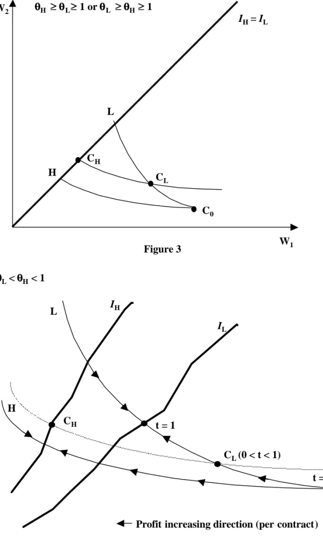
When both types are pessimistic (min{θH, θL} ≥ 1), overinsurance being precluded,
the efficient coverage for both is full insurance. Stiglitz’ equilibrium configuration (separation of the types, full coverage for one of the types and partial coverage for the other) again applies. This situation is shown in Figure 3.
INSERT FIGURE 3 HERE
However, for a proportion of L close to 1, a minor difference has to be mentioned. It appears directly, from point 2 of Theorem 1 that if θL > 1, then threshold ξ1
is strictly lower than 1, which means that types are pooled on CL, the contract
extracting maximal rent on type L. This absence of discrimination of the types would not remain true if overinsurance was permitted.
5.2
At least one optimistic type
Equilibrium configurations specific to our model appear when at least one of the types is optimistic (θH or θL is lower than 1), especially where:
• All types may obtain partial coverage; • A pooling contract may be an equilibrium. This definition is used in the following.
Definition 1 A type i (i = H, L) is over-covered (under-covered) by a contract (W1, W2) if the coverage offered (measured by u0(W1)/u0(W2)) is larger (respectively
smaller) than the efficient one θi.
5.2.1 L more optimistic than H (θL< θH and θL < 1)
In this case, I(θL) is below I(θH) and below the full insurance line. If θH < 1,
absent, full coverage would be profit maximizing for neither of the two types. This case is significant in practice since beliefs and probabilities are positively correlated: type H represents high risk in terms of preferences and in terms of cost.
The general characteristics of the equilibrium configurations are as follows.
Proposition 2 If θL < θH and θL < 1, then:
1. Types are always separated.
2. Type H obtains optimal insurance:
(a) if θH ≥ 1, type H receives full coverage
(b) if θH < 1, optimal coverage is partial.
3. Type L never gets efficient insurance (except if λH = 0).
4. There is ξ0 (0 < ξ0 < 1) such that type L is offered insurance if and only if λL > ξ0, and then, type L’s coverage is continuously strictly increasing with
respect to λL.
To obtain the first two points, we start from a contract on the participation constraint of L and try to determine the most profitable contract for H which is incentive compatible. This contract corresponds to an efficient contract (on I(θH))
such that type H consumers are indifferent between their contract and type L’s contract. If θH ≥ 1, then efficient contracts for type H correspond to full coverage
and if θH < 1, they correspond to partial coverage. The latter situation is depicted
on Figure 4.
INSERT FIGURE 4 HERE
The other points of the proposition are direct consequences of Theorem 1. Note that, stated as it is, the proposition is true only if the two types participated if they were alone on the market: min{θH , θL} ≥ θ with θ ≡ u0(W0)/u0(W0− d). If
neither type participated, then the market would not be active at all. If type L only did not participate, there is de facto no adverse selection and type H is optimally insured.
5.2.2 H more optimistic than L (θL> θH and θH < 1)
This configuration corresponds to a situation when the low belief type’s optimal coverage is higher. Type H can objectively be the low risk, though we don’t think that this negative correlation between beliefs and risks is the most realistic situation. The characterization of equilibria in this situation is given in the following propo-sition.
Proposition 3 Assume both types need insurance (θL> θand θH > θ). If θL> θH
and θH < 1, then there are thresholds denoted by ξ0, ξ0 and ξ1 with 0 < ξ0 < ξ0 < ξ1
such that
1. If λL < ξ0 then (a) types are separated, (b) type H obtains an efficient coverage,
(c) type L is offered insurance if and only if λL > ξ0 (coverage is increasing
with respect to λL).
2. If λL= ξ0 then (a) types are pooled, (b) type H obtains efficient coverage.
3. If ξ0 < λL < ξ1 then (a) types are pooled, (b) neither type obtains efficient
coverage, (c) coverage of the pooling contract is strictly increasing with respect to λL.
4. If λL≥ ξ1 then types are pooled on CL, type L’s profit maximizing insurance.
The origin of optimality of the pooling contract is as follows: on the one hand self-selection constraints force type L to receive less coverage, but on the other hand, type L more highly values coverage. This conflict can only be solved with pooling, which is impossible in Stiglitz’ model.
This pooling occurs only if the proportion of type L is sufficiently large, i.e. if the insurer considers that leaving rents to type H to gain profits on type L is valuable. Under this condition, as it is difficult to separate types, it is therefore optimal to accept that type H receives over-coverage and type L under-coverage. More precisely, when the proportion of type L becomes high, the monopoly is induced to approach CL as close as possible. Given that θH < θL, contracts that give more
than CL, but such contracts are also more attractive for type L than CL
(single-crossing condition). The monopoly is forced to pool types on CL.
INSERT FIGURE 5 HERE
The participation problem is somewhat more complex here than in paragraph 5.2.1. If, in the absence of adverse selection, type H did not participate whereas type Lparticipated, the optimal offer to the latter always attracts the former. In this case where participation constraints matter, we obtain a truncated version of the previous proposition: only some of the equilibrium configurations remain. Namely, the fact that negative insurance is not allowed creates the possibility that no insurance at all be offered in equilibrium, though one type at least (here L) would like to obtain some form thereof. This occurs for high proportions of type H.
The main results in this case, obtained directly from Theorem 1 are as follows:
• there is a threshold ξ0 such that if λL ≤ ξ0 then no insurance is offered in
equilibrium.
• for λL > ξ0, there is ξ1 such that if ξ0 < λL < ξ1, then types are pooled and
neither type gets optimal insurance, and for λL≥ ξ1,types are pooled on type
L’s optimal insurance.
The result is that, provided the type requiring insurance (here L) is sufficiently numerous, then the other type can easily be subsidized through a unique insurance contract offered to all.
6
Conclusion
To summarize, two categories of situations can be distinguished: “pessimism ratios” (θL and θH) and costs are either positively or negatively correlated. In the case of
positive correlation, results are, by and large, quite similar to those of Stiglitz: the high risk wants and receives more coverage; adverse selection forces a rationing of the low risk in terms of the quality of insurance, meaning that the low risk remains less covered.
The case of negative correlation is less standard and still significant in practice: even if people are aware of their relative riskiness (qL < qH), pL< pHand θL> θH at
the same time is a plausible situation. In the absence of adverse selection, everybody would be proposed a fair rate and low risk people would undertake more insurance. In a situation of adverse selection, this possibility is precluded by the propensity of the high risk to prefer cheaper contracts. In equilibrium, we have the strikingly robust prediction that the optimal offer of the monopolistic insurer can be a pooling contract. In Landsberger and Meilijson [5], a pooling, if it is optimal, systematically offers full insurance for all; here a pooling is typically optimal for nobody, since it represents a compromise between covering low risk consumers sufficiently (because it is socially desirable) while not covering high risk consumers too much (because it is socially costly).
The introduction of a gap between beliefs and probabilities in an insurance model with adverse selection, in addition to making the model closer to reality, explains a wider range of optimal configurations. For given true probabilities, the quality of the information consumers use to make their choice is a parameter that should not be overlooked. If our model is more realistic than the standard approach as we know it from Rothschild and Stiglitz [7] or Stiglitz [10], whether the disparity comes from a lack of information on the part of the public or a violation of the independence axiom is the critical question. Our paper remains agnostic with respect to the various interpretations of non-expected utility that could be given. In a more comprehensive game, an effective public policy (or the strategy of a monopoly) should be founded on a clear identification of the origin of the observed behavior.
A
Appendix
A.1
Proof of Lemma 1
Uniqueness. Assume that there are two different solutions (CL, CH) and (CL0, CH0 ).
Define a pair of randomized contracts (Cε
L, CHε)with 0 < ε < 1 in the following way:
with Cε
L,whether there is an accident or not, the policyholder receives the wealth
prescribed by contract CL with probability ε and wealth prescribed by contract CL0
with probability 1−ε. This randomization is consistent with incentive compatibility and doesn’t change the expected profit of the insurer (each pair gives the same value of the objective). The following explains why we used (temporarily) contracts that were not permitted in C.
What is interesting here is that the contingent lotteries are perceived identically by different types: e.g., conditional on loss, CLε is worth εu(WL2) + (1− ε)u(WL20 ),
with WL2 (WL20 ) the wealth in case of loss for contract CL (CL0). This lottery can be
replaced by its certainty equivalent Wε
L2,where u(WL2ε ) = εu(WL2) + (1− ε)u(WL20 ).
When implemented on all conditional lotteries, this replacement preserves incen-tive compatibility and creates deterministic contracts. Due to the concavity of the agents’ utility functions, this transformation yields a pair of contracts in C which is more profitable than those with which we started. This proves that two optima were not different.
1. Assume that every type strictly prefers its contract to the uninsured posi-tion. (i) If both types are indifferent between the two contracts, then the contracts are identical (single-crossing property). By lowering (slightly enough) the reim-bursement in case of accident (or by increasing the premium), we can maintain participation and increase profits, which contradicts that profits were maximal. (ii) If a type strictly prefers its contract, we make the same operation on this contract, so that incentives are not reversed. This also contradicts that profits were maximal. In consequence, one type’s rationality constraint at least is binding. The single-crossing property and the fact that negative insurances are forbidden ensure that this type is L.
2. (i) Assume now that every type strictly prefers its own contract to the con-tract designed for the other type. Each type is thus necessarily on its rationality constraints, else the type which is not constrained would see its benefits cut (profits would increase and participation would be preserved). The single-crossing property helps once more: each type being indifferent between its contract and no insurance, then necessarily type L gets no insurance. This is a contradiction with the assump-tion that each type strictly prefers its contract. (ii) There is a type at least which is indifferent between both contracts. If type H strictly prefers its contract, we know that type H is strictly better off with this contract than without insurance. Therefore, by lowering reimbursement slightly in case of accident, we maintain par-ticipation and type H will not switch to type L’s contract. The aggravation of type H’s contract in terms of first-order stochastic dominance also ensures that type L does not switch.
A.2
Proof of Theorem 1
We need the following lemma.
Lemma 2 πL(·) and πH(·) are C1(derivatives exist and are continuous) and π0L(·) >
0 and π0
H(·) < 0.
Proof. Equations in (15) are linear with respect to u(W1(t))and u(W2(t)).Since
qL 6= qH and u is strictly monotonic and continuous, the solution exists, is unique
and has a continuous derivative with respect to t. Given that
πL(t) = (1− pL) (W0− W1(t)) + pL(W0− d − W2(t)), (19)
it follows that
π0L(t) =−(1 − pL)W10(t)− pLW20(t). (20)
Differentiating the first equation in (15) leads to
W10(t) =−
qLu0(W2(t))
(1− qL) u0(W1(t))
W20(t), (21)
which we plug in the second equation (after differentiation) to get W0
2(t) > 0 and
thus W0
1(t) < 0. By a simple calculation, from (15) and (20), we obtain:
sgn {π0L(t)} = sgn ½ W20(t)[u 0(W 2(t)) u0(W1(t))− 1 θL ] ¾ . (22)
For the chosen parameterization, CL(t)is always on or below I(θL)(under-coverage).
This gives the sign of the right-hand side, and the result: π0
L(·) > 0 for all t ∈ (0, 1)
and is continuously differentiable with respect to t; moreover, π0
L(1) = (>)0 if and
only if θL≤ (>)1.
From the parametrization, πH(t) is the value function of the following program:
πH(t) = max (W1,W2)∈C
(1− pH) (W0− W1) + pH(W0− d − W2) (23)
subject to (17).
We rewrite the program as follows:
πH(x, y) = max U1,U2
subject to
(1− qL) U1+ qLU2 ≤ x, (25)
(1− qH) U1+ qHU2 ≥ y. (26)
After this transformation, the objective function is still concave (u concave ⇒ u−1
convex ⇒ −u−1 concave). Constraints are linear and form a convex set. Hence, the
solution of the program exists and is unique for every x and y. We transform the pro-gram to make it linear in probabilities by allowing random W1 and W2 (the support
is assumed compact but sufficiently large). Hence the objective becomes concave and the constraints convex. Moreover, the constraint qualification requirement is always satisfied since the objective and the constraints are linearly independent: the solution exists and is necessarily unique for every x and y. It follows that πH(x, y)is
differentiable with respect to x and y. Replacing x by (1−qL) u(W1(t))+qLu(W2(t))
and y by (1 −qH) u(W1(t)) + qHu(W2(t)), which are both continuously differentiable
functions of t (see the first part of the proof), yields that πH(t) is continuously
dif-ferentiable. π0
H(t) < 0 comes directly from the fact that πH(t) and πL(t) vary in
opposite directions and we proved that π0
L(t) > 0.
We can now prove our Theorem.
1. Continuity comes from a variety of the Theorem of the Maximum. As-sume that there is a value of λL denoted by ξ where t∗(·) is not continuous,
mean-ing that there is a sequence (ξs)s≥0 converging to ξ (the limit exists and is finite
since t∗(·) takes its values in a compact set), such that lim
s→+∞t∗(ξs) < t∗(ξ) or
lims→+∞t∗(ξ
s) > t∗(ξ). As the reasoning is essentially the same for the two
differ-ent case, we argue as if the first inequality were fulfilled. We denote the limit by t∞ < t∗(ξ). Consider now the value of the objective for ξs: ξs πL(t∗(ξs)) + (1−
ξs) πH(t∗(ξs)). The limit of this value when s goes to infinity is necessarily equal to
ξ πL(t∗(ξ)) + (1− ξ) πH(t∗(ξ)) (else, there is a contradiction with the fact that the
objective is a continuous function). Hence, two values (t∞ and t∗(ξ)) maximize the
objective given ξ. A contradiction with uniqueness. This proves the continuity of t∗(·).
3. (3 is proved before 2) Monotonicity. We know from the symmetric information case that if λL= 0, then t∗ = 0, and if λL= 1, then t∗ = 1. Continuity ensures that
interior solution can be expressed:
λLπ0L(t∗(λL)) + (1− λL) π0H(t∗(λL)) = 0 (27)
Thus, any t ∈]0, 1[ determines entirely the corresponding λL as:
λL 1− λL =−π 0 H(t) π0 L(t) > 0 (28)
Consequently, two different ratios cannot correspond to the same menu if 0 < t∗ < 1.
This proves that t∗(·) is a strictly increasing function wherever its value differs from
0 or 1.
2. Corner Solution. From (28), we see that ξ0 such that ξ0
1−ξ0 =−π
0
H(0)/π0L(0)
has the announced properties. The offer t∗ = 1 will be made for λL ≥ ξ1 such that 1−ξ1
ξ1 = −π0L(1)/π0H(1). This and (22) imply that ξ1 < 1 if θL > 1 and ξ1 = 1 if
θL ≤ 1. Remark also that the monotonicity of t∗ proved in the previous paragraph
proves that ξ1 > ξ0.
A.3
Proof of Proposition 3
The intersection between the reservation indifference curve of type L, and the opti-mal insurance set I(θH)is located in the parameterized domain {CL(t) : t∈ (0, 1)}
since θL > θH. Therefore, this point corresponds to a certain t ∈ (0, 1), denoted
by t0. We define ξ0 such that ξ0
1−ξ0 ≡ −π0H(t0)/π0L(t0). The order between ξ0 and ξ1
comes from the monotonicity of the ratio of marginal profits (Theorem 1).
If λL < ξ0, the situation is similar to that of Proposition 2, which explains 1. If
λL > ξ0, the insurer is constrained to pool the two types. Indeed, the offer made
to type L, say CL, gives more coverage than desired (at the optimum) by type H.
As a consequence of Lemma 1, the offer to type H, say CH, is equivalent to CL
for type L. If CH covers more than CL, then the insurer could increase its profit
by offering only CL (CL over-covers type H, but less). If CH covers less than CL,
then the single-crossing property ensures that type L prefers CH to CL,which is not
incentive compatible. Types are therefore necessarily pooled. The rest of the comparative statics derives from Theorem 1.
References
[1] Chiappori, P.A., Salanié, B.: Testing for asymmetric information in insurance markets. Journal of Political Economy 108, 56-78 (2000)
[2] Jaffray, J.Y.: Généralisation du critère de l’utilité espérée aux choix dans l’incertain régulier. Recherche Opérationelle 23, 237-267 (1989)
[3] Jeleva, M.: Demand for insurance with imprecise probabilities. Finance 18, 101-114 (1997)
[4] Landsberger, M., Meilijson, I.: Monopoly insurance under adverse selection when agents differ in risk aversion. Journal of Economic Theory 63, 392-407 (1994)
[5] Landsberger, M., Meilijson, I.: A general model of insurance under adverse selection. Economic Theory 14, 331-352 (1999)
[6] Quiggin, J.: A theory of anticipated utility. Journal of Economic Behavior and Organization 3, 324-343 (1982)
[7] Rothschild, M., Stiglitz, J.: Equilibrium in competitive insurance markets: an essay on the economics of imperfect information. Quarterly Journal of Eco-nomics 90, 629-649 (1976)
[8] Savage, L.: The foundation of statistics. New York: J. Wiley 1954
[9] Schmeidler, D.: Subjective probability and expected utility without additivity. Econometrica 57, 571-587 (1989)
[10] Stiglitz, J.: Monopoly, Non-linear pricing and imperfect information: the in-surance market. Review of Economic Studies 44, 407-30 (1977)
[11] Villeneuve, B.: The consequences for a monopolistic insurance firm of eval-uating risk better than customers: the adverse selection hypothesis reversed. Geneva Papers on Risk and Insurance Theory 25, 65-79 (2000)
W2 W1 C0 I(θ), θ < 1θ), θ < 1 Figure 1 I(θ), θ ≥≥ 11θ), θ C (θ < 1)θ < 1) C(θ θ ≥≥ 1)1) W2 W1 C0 IH IL θθL<θθH< 1 t = 0 t = 1 L H CL(t) CH(t) π=0
Figure 3 W2 W1 L H C0 CH CL θθH ≥≥ θθL≥≥ 1 or θθL ≥≥ θθH ≥≥ 1 IH = IL IL IH L H t = 1 CL (0 < t < 1) CH
Profit increasing direction (per contract)
Figure 4
t = 0 θθL< θθH< 1
IL
IH
L
H
t = 1
Profit increasing direction (per contract) t’(corresp. to ξ’)
Pooling contract
Figure 5
t = 0 11> θθL> θθH