de l’Université de recherche Paris Sciences et Lettres
PSL Research University
Préparée à l’Université Paris Dauphine
Quelques propriétés et applications du contrôle
en temps minimal
École Doctorale de Dauphine — ED 543
Spécialité
Sciences
Soutenue par
Michaël ORIEUX
le 27/11/2018
Dirigée par
Jacques Féjoz
& Jean-Baptiste Caillau
COMPOSITION DU JURY :
M. Jacques FEJOZ Université Paris Dauphine Directeur de thèse
M. Jean-Baptiste CAILLAU Université Côte d’Azur Co-Directeur de thèse
M. Andrei AGRACHEV SISSA
Rapporteur
M. Jean-Pierre MARCO
Université Pierre et Marie Curie Rapporteur
M. Guillaume CARLIER Université Paris Dauphine Membre du jury
Mme Francesca CHITTARO Université de Toulon
Membre du jury
M. Robert ROUSSARIE Université de Bourgogne
Baptiste Caillau et Jacques Féjoz. Ils ont su m’encadrer et me donner la bonne direction tout en me laissant l’espace de m’épanouir, merci à vous deux.
Je tiens également à remercier chaleureusement mes deux rapporteurs, Andrei Agrachev et Jean Pierre Marco, pour leur travail et leurs remarques constructives sur le manuscrit. Un grand merci aussi à Robert Roussarie et Thierry Combot pour leur aide, ce fut un plaisir de travailler avec vous. Je tiens également à remercier Francesca Chittaro et Guillaume Carlier pour avoir accepter de faire partie de mon jury. Enfin, merci à Olivier et Vincent, qui se sont toujours soucié du sort des doctorants.
Ma famille et son indéfectible soutient ont également été indispensable ! Merci à ma mère et mon père, tout spécialement, les retours dans notre maison bretonne ont été aussi bien reposants que stimulants. Merci à Jean Claude et Christianne, pour m’avoir fournis un deuxième endroit que j’ai pu appeler chez moi. Un grand merci à mon frangin pour son soutien ! Et aux amis de Perpignan, Guillaume, Cailloux et Beno.
Je tiens bien entendu à remercier chaleureusement Pascale, tonton Michel, et leurs magnifiques filles, Lola et Nina ! J’espère bien que les soirées dégustations de rhum chez vous ne cesseront jamais.
***
Ces remerciements vont devenir beaucoup plus informel !
Mes acolytes de toujours, Grognini et Pedro, doivent parcourir ces lignes en se demandant quand leur nom apparaîtra (Ne dites pas non je vous connais !). Merci tout particulièrement à Julien pour avoir écrit les pires remerciements de thèse que j’ai pu lire ! Votre présence, nos conversations et autres cabotinages, ont insufflé de la joie à ces trois années, je ne sais pas où j’en serais sans vous (mais surement beaucoup plus loin !). Ce triangle amoureux est le théatre d’une saine émulation. Peu de gens, il me semble, ont la chance de partager une telle amitié. Merci aussi bien sur à Mr. Groburu, mon indépendantiste Basque préféré, et à Jojo le Galopin.
Merci aussi à tous les amis du laboratoire, Arnaud qui fut mon acolyte favoris (que vas tu devenir quand je ne serai plus la pour t’empêcher de travailler ??), Camille, le Grand Maître du LATEX, Qun mon frère tmtc, Raphaël & Raphaël, Luca,
autant que moi.
I’d obviously like to give a warm thank you to the whole Barcelona team : Eva, Cedric and Roisin, loved this time together, math with you is something else entirely! Thanks also to the conferences buddies! Jeremy, Sara, Gladstone, Nathan, Maria, those were fun times.
Passons aux copains de Cachan, votre présence a elle aussi été salvatrice ! Merci à Léa, tu seras toujours ma naine rousse préférée, Clément, Martine, Margot, Nicolas, Théophile et tous les autres. Je reviendrai (avec du rouy). Certains d’entre vous y passerons aussi, j’ai hate d’assister à vos soutenances ! Merci aussi à Lucile, d’une certaine manière, cette thèse a commencé, et s’est fini, avec toi (presque).
Merci également aux sympathiques plongeurs, et tout spécialement à Claire, Linh, Théo, Luc, Olivia, Olive et tous les autres bien sur, je vous aime, nous retournerons buller ensemble.
Une grosse pensée enfin pour mes amis de Montpellier, Brice, Jackson, Tonio, Quentin, Farouk, on se suit depuis longtemps, et vous êtes toujours aussi bêtes, ça fait plaisir à voir.
Spéciale dédicace à ma petite Marjolaine, comment pourrais-je t’oublier ! Ces remerciements ne pourrait être complet sans mentionner Charles Henri et Thomas. J’aurai tellement aimé que vous puissiez être la, les gars. Je pense à vous.
Introduction 7
Introduction 17
1 Singularities of minimum time control for mechanical systems 27 1.1 Quick introduction to geometric control & necessary conditions for
optimality . . . 30
1.1.1 Controllability. . . 30
1.1.2 Geometric optimal control . . . 32
1.2 Singularities of minimum time control for mechanical systems . . . 36
1.2.1 Setting . . . 37
1.2.2 Stratification of the extremal flow . . . 38
1.2.3 Regular-singular transition . . . 47
1.2.4 Application to mechanical systems . . . 54
1.3 Conclusion and perspectives . . . 58
2 Singularities of minimum time control-affine systems 61 2.1 Setting . . . 64
2.2 The bifurcation formulation . . . 67
2.2.1 The case Σ´. . . 68
2.2.2 The case Σ`. . . 68
2.2.3 The bifurcation α “ 0: case Σ0. . . 69
2.3 Conclusion . . . 81
3 Sufficient conditions for optimality of minimum time control-affine systems 83 3.1 The smooth theory . . . 87
3.3 Proof of theorem 3.2 . . . 90
3.4 Regularity of the field of extremal . . . 93
3.5 Conclusion and perspectives . . . 94
4 Liouville integrability and optimal control systems 97 4.1 Liouville-integrability and algebraic obstructions . . . 100
4.1.1 Integrability of Hamiltonian systems and optimal control theory . . . 100
4.1.2 Introduction to Galois Differential Theory . . . 104
4.2 Integrability and its obstructions in Hamiltonian systems coming from optimal control . . . 110
4.2.1 Setting . . . 111
4.2.2 Proof of Theorem 4.9 . . . 115
4.3 Conclusion and perspectives . . . 119
Les problèmes de contrôle optimal sont à la croisée des chemins des systèmes dynamiques et de l’optimisation. Ces points de vue très différents ont tous deux de l’intérêt. D’un côté, on peut formuler le problème comme ceci : Comment peut-on trouver (ou prouver l’existence / unicité) des solutions d’une équation différentielle non autonome minimisant un certain coût, fixé à l’avance ? Selon l’autre point de vue, la question ressemblerait plutôt à : Comment résoudre un problème d’optimisation avec une contrainte dynamique ? Dans tous les cas ces problèmes sont de la forme suivante :
$ ’ ’ & ’ ’ % 9 x “ f px, uq, t P r0, tfs xp0q “ x0, xptfq “ xf Cpuq “ştf 0 ϕpxptq, uptqqdt Ñ min . (OC )
où f est une famille de champs de vecteurs paramétrés par u P U , et U est un ensemble contraignant le contrôle, sur une variété M . Le choix, pour chaque temps t, d’un "meilleur" uptq P U , quand cela est possible, mène à un couple minimisant px, uq. Dans la seconde moitié du vingtième siècle, des techniques de nature géométrique ont été élaborées pour étudier ces problèmes. Nous rap-pellerons quelques notions mais ne ferons pas de tour complet de ces méthodes et nous renvoyons au livre [4] pour une présentation moderne. Elles reposent davan-tage sur l’aspect dynamique et sont plus proches des techniques employées dans cette discipline ainsi que de celles de la géométrie Riemannienne, par opposition aux méthodes venant du domaine de l’optimisation. La géométrie Riemannienne est de fait un cas particulier de géométrie sous Riemannienne, où la dynamique est linéaire en le contrôle, et la distribution de champs en question génère linéairement l’espace tangent en chaque point. Ces problèmes peuvent être formulés comme (OC), ϕ étant la norme au carré du contrôle.
Le coût est bien entendu d’une importance capitale, et le comportement des solutions de pOCq varie de manière drastique quand ce dernier change, en
conser-vant la même dynamique. Cette thèse se concentre sur les problèmes en temps optimal, où le but est d’aller d’une position initiale x0 à une position finale xf
en minimisant le temps d’arrivée. Ces problèmes sont étudiés dans le cadre où la dynamique initiale dépend du contrôle de manière affine. Ces systèmes, de la forme 9 x “ F0pxq ` m ÿ i“1 uiFipxq (Aff )
restent très généraux : ils modélisent par exemple les système mécaniques et la plupart des problèmes de contrôle survenant dans la nature (modélisés par des EDO). Les systèmes mécaniques constituent l’application principale des travaux présentés ici, et seront notamment traités en détail certains système issus de la mécanique spatiale : le problème de transfert d’orbite, avec deux ou trois corps, au chapitre I, et IV.
Les méthodes géométriques sont tout indiquées pour l’étude des systèmes de contrôle affine. En effet, la plupart des propriétés de ces systèmes sont encodés dans les champs de vecteurs Fi supportant la dynamique, et dans leurs algèbres
de Lie. La structure de ces algèbres
LiexpF0, F1, . . . , Fmq, x P M
est primordiale, et de nombreux résultats classiques de contrôlabilité sont là pour en témoigner. L’intuition peut être donnée par un exemple célèbre : le prob-lème consistant à garer sa voiture en créneau. Au vu des contraintes (dites, non holonomes), on ne peut se placer en face de la place en question et se déplacer perpendiculairement dans la direction voulue : aucun des champs de vecteurs ne permet ce mouvement. Il faut au contraire manœuvrer, et faire une série de mou-vements pour accéder à ce déplacement : c’est une direction donnée par le crochet de Lie de ces champs, [37]. Cette structure reste très importante dans les prob-lèmes de contrôle optimal. Tout au long de cette thèse, nous aurons besoin d’une hypothèse générique sur l’algèbre de Lie des champs, voir pAq au chapitre I, section 1.2. Le choix de minimiser le temps final est très particulier parmi tous les coûts disponibles, il est plus intimement lié à la dynamique initiale que les autres. En effet, selon le Principe du Maximum de Pontrjagin, les trajectoires optimales sont les projections des solutions d’un système Hamiltonien défini sur le cotangent de l’espace d’état par Hpx, p, p0, uq “ xp, f px, uqy ` p0ϕpx, uq. Pour les problèmes en
temps optimal, ϕ “ 1, et sa présence dans le pseudo-Hamiltonien ne change rien aux courbes intégrales. On a alors affaire au relevé canonique au cotangent de la dynamique initiale. C’est encore plus marquant avec des systèmes de contrôle
affine, où F0, le drift, est le champ de la dynamique non contrôlée : Hpx, p, uq “ H0px, pq ` m ÿ i“1 uiHipx, pq. (P-H)
Le hamiltonien est alors aussi affine en le contrôle et c’est une perturbation du relevé de la dynamique non contrôlée, si tant est qu’on considère des contrôles as-sez petits. Pour être plus précis, le Principe du Maximum affirme qu’il existe une courbe absolument continue pptq dans le fibré cotangent et une constante négative
p0, telles que H est maximum le long de pxptq, pptq, uptqq parmi toutes les autres valeurs possibles pour le contrôle. Il est alors tentant de définir (quand il ex-iste) Hmax
px, pq “ maxuPUHpx, p, uq, et d’étudier les solutions du système XHmax.
On appelle extrémales ces courbes px, pq, et leur projection x est une trajectoire extrémale. Quand le temps final n’est pas fixé, comme pour les problèmes en temps minimal, le P.M.P fournit une condition supplémentaire : H ” 0 le long des extrémales, ce qui nous donne encore H “ ´p0 pour le temps optimal avec
Hpx, pq “ xp, f px, uqy. Les extrémales dites normales correspondent au cas p0 ‰ 0, c’est le cas intuitif et général, tandis que quand p0
“ 0 on dit que l’extrémale est
anormale. Quand on s’intéresse aux systèmes en temps minimal, les extrémales
normales et anormales sont solutions de la même équation différentielle, mais les normales correspondent aux niveaux H ą 0 et les anormales sont sur H “ 0. L’étude des anormales est une des difficultés principales en contrôle optimal ; mis à part au chapitre III, nos résultats restent valides aussi bien dans le cas normal, qu’anormal.
Sans conditions supplémentaires sur le système (OC), Hmax n’a aucune raison
d’être régulier ou même bien défini. Le sujet principal de cette thèse est l’étude des singularités générées par cette condition de maximisation pour les systèmes en temps optimal. Nous nous intéresserons à plusieurs aspects et conséquences de ces singularités, selon différents points de vue. Une première conséquence, immédiate, est donnée par le comportement du flot extrémal au voisinage de ces singularités; nous verrons aux chapitres I et II qu’il peut y avoir bifurcation sur le lieu des points singuliers. La non-optimalité des extrémales, même locale, en est une autre. Nous verrons une condition permettant d’obtenir l’optimalité locale au chapitre III. Enfin, ces singularités peuvent aussi induire une absence d’intégrabilité, au sens de Liouville, pour le système Hamiltonien: le problème de Kepler, ainsi que son relevé au cotangent, sont des systèmes intégrables, pourtant nous montrerons au chapitre IV que son contrôle en temps minimal donne lieu à un système non intégrable.
Ces singularités coïncident avec les discontinuités du contrôle optimal (ou au moins, extrémal), appelé switchings. Eux mêmes se produisent lorsque prendre le maximum du pseudo-Hamiltonien sur les valeurs possibles du contrôle n’a pas de sens ou ne définit pas un u unique. L’Hamiltonien maximisé de (P-H) est
Hmaxpzq “ H0pzq ` dm ÿ i“1 H2 ipzq, z P T˚M (Hmax)
(voir le calcul au chapitre I, section 1.1.). Les singularités se produisent clairement sur le lieu singulier
Σ “ tH1 “ ¨ ¨ ¨ “ Hm “ 0u.
Le but de ce travail est donc la compréhension de ces singularités et de leurs conséquences, sous les différents angles mentionnés ci dessus. Une inspiration majeure a ainsi été l’article fondateur d’Ekeland [28]. Nous donnons maintenant un résumé des différents chapitres.
Chapitre I: Les singularités du contrôle en
temps minimal des systèmes mécaniques
Le but de ce chapitre est l’étude du flot extrémal des systèmes de contrôles affine en temps minimal, dans un cas particulier des singularités possibles qui contient les systèmes mécaniques. Ce cas correspond à la zone Σ´ défini en1.2.2. C’est à
dire les systèmes de la forme :
q ` ∇V pqq “ u,
ou l’état q appartient à une variété de dimension 4 (ou 2n jusqu’à la section1.2.3),
V est une fonction lisse sur M (le potentiel) et u le contrôle : une force, que l’on
choisit de façon à ce que l’état parte d’une position-vitesse initiale, et arrive à une position-vitesse finale, le plus rapidement possible. Ce problème ne serait pas bien posé sans borne sur le contrôle, et on le contraint ici à être dans une boule Euclidienne. De manière informelle, nous montrons que les singularités dans ce cas sont régulières, et que le flot est lisse par morceaux. Le chapitre débute par des rappels sur les notions de base et définitions de théorie du contrôle (contrôlabilité, ensemble accessible), puis nous introduisons les problèmes de contrôle optimal et les conditions nécessaires d’optimalité. En particulier, un énoncé précis est donné pour le Principe du Maximum de Pontrjagin avec temps final libre. Nous
détaillons ensuite le calcul du hamiltonien vrai, au sens où il ne dépend plus du contrôle, dont les extrémales sont des relevés au cotangent des solutions optimales de (OC). Quelques exemples importants, qui seront repris tout au long de cette thèse, sont ensuite donnés.
Nous procédons ensuite en section 1.2.2 à une régularisation du champ de vecteurs donné par XHmax d’après un éclatement polaire initié dans [2]. Ceci
conduit à un résultat d’existence et d’unicité pour le flot extrémal, ainsi qu’à la construction d’une stratification sur laquelle le flot s’avère être lisse. La strate
S1 est celle de codimension 1, c’est aussi celle composée des conditions initiales
menant au lieu singulier. Elle est construite comme la variété stable globale à une variété N , normalement hyperbolique pour le flot régularisé et contenue dans Σ. Ce caractère normalement hyperbolique ainsi que le fait que la dynamique soit triviale sur la variété N nous permet de conclure quand à la régularité des strates et du flot. Nous démontrons également la continuité du flot extrémal.
Dans la section suivante en1.2.3, une étude de l’application de transition entre les strates est menée. Nous donnons une forme normale pour le flot, permettant de définir deux sections transverses aux strates. La forme normale est d’abord formelle, donnée par une série en les monômes résonants (ici, les monômes qui commutent avec la partie linéaire du flot), et l’on prouve une généralisation du théorème de Takens en ce sens. Il est alors possible de réaliser ces séries par des fonctions lisses, par le théorème de Malgrange (qui généralise celui de Borel, sur les séries réelles). Cette forme normale permet d’obtenir la régularité voulue, grâce à un éclatement projectif défini en fin de section. Nous obtenons des singularités en
d ln d pour l’application de transition, où d représente la distance à la strate S1.
Enfin, la dernière section de ce chapitre est consacrée à l’application aux sys-tèmes mécaniques, puis va plus loin pour les problèmes de transfert d’orbite à deux ou trois corps. Ces problèmes ont une structure très particulière : la distribution de champs pF1, F2q commute. Ceci implique que les switchs sont en fait des
rota-tions instantanées d’un angle π du contrôle. La fonction de switch, fonction qui s’annule aux temps de switchs, vérifie une équation différentielle linéaire d’ordre deux, et nous pouvons utiliser les théorèmes de comparaison à la Sturm pour con-trôler l’intervalle de temps entre deux singularités. Dans le cas des problèmes de mécanique spatiale, nous donnons une borne supérieure sur le nombre de switchs pouvant arriver au cours d’un transfert en fonction de la distance aux collisions (les chocs avec les autres corps).
Chapitre II: Les singularités des systèmes
affines en temps minimal
Le chapitre précédent a laissé ouverte la question des singularités se produisant en dehors de Σ´, dans le reste du lieu singulier. Ces singularités ne peuvent pas se
produire pour les systèmes provenant de la seconde loi de Newton, comme il est montré en section 1.2.4. Nous répondons néanmoins à cette question de manière complète pour les systèmes de contrôle à double entrée sur les variétés de dimension 4 (avec un contrôle contenu dans une boule Euclidienne). Les strates stable et instable construites au chapitre I fusionnent en un point d’équilibre nilpotent dans Σ pour le système régularisé. L’analyse des switchs et du flot extrémal en ce point requiert ainsi d’autres outils. Nous commençons, en section 2.2, par unifier les points de vue en donnant un système à paramètre α, contenant notre problème. A la bifurcation α “ 0, dans (2.2.3), se produit la rencontre des variétés stable et instable.
Nous donnons ensuite une description du flot singulier - flot contenu dans Σ - comme le flot d’un certain Hamiltonien lisse, et une comparaison est faite avec le cas, plus simple, du système mono-entrée, quand le contrôle est scalaire. Nous discutons aussi du même système avec une contrainte différente sur le contrôle : quand U “ r´1, 1sm. De nombreuses études ont été menées dans ce contexte, et
nos singularités peuvent être apparentées à des switchs doubles, mais on ne peut, en pratique, les traiter de la même manière que dans [48]. Une extrémale dite bang est en essence une extrémale qui reste en dehors du lieu singulier, et son contrôle associé est lisse. Une concaténation d’extrémales bang est appelée bang-bang, c’est le cas des extrémales de la strate S1 sur un temps plus grand que le temps
de switch. En dehors de la zone Σ´ un flot existe dans le lieu singulier, on dit que
les extrémales correspondantes sont singulières, et il peut exister des connexions bang-singulière.
Nous présentons d’abord le cas le plus simple, celui ou les extrémales n’entrent pas en contact avec le lieu singulier ; cette zone est notée Σ`, et une simple
es-timation à la Gronwall suffit. En section 2.2.3, nous traitons la bifurcation, et la fusion des variétés stable et instable. Nous procédons à un éclatement quasi-homogène pour étudier l’équilibre nilpotent du champs régularisé. Cet éclatement, introduit par Dumortier dans [27], consiste à trouver les bons poids pour chaque coordonnée, de façon à ce que l’anisotropie désingularise le système, ce qu’un seul éclatement en coordonnées sphériques classiques n’aurait pu effectuer. Une
fois l’équilibre désingularisé, nous procédons à l’étude du système éclaté sur la (demi-)sphère, et obtenons cinq nouveaux équilibres, tous hyperboliques ou semi-hyperboliques. Cette étude est grandement facilitée par la dimension deux : nous pouvons utiliser la panoplie de résultats existants dans le plan. Le théorème de Poincaré-Bendixson nous permet de relier les variétés instables de ces équilibres avec les variétés instables des autres, si l’on prouve l’absence de trajectoires péri-odiques. Nous parvenons à le démontrer en utilisant la formule de Stockes sur un domaine bien choisi de l’hémisphère transverse au champ. Nous exhibons, dans la moitié des cas une direction stable provenant de l’extérieur de la sphère, prouvant au passage le théorème 2.2 sur l’existence de switchs dans ce cas. Deux possibil-ités se présentent alors : selon le signe du crochet de Poisson des relevés des deux champs H12, le contrôle associé à l’extrémale peut être continu ou présenter une
π-singularité. Une analyse similaire à celle du chapitre I permet alors d’obtenir
également une stratification sur laquelle le flot est lisse. Avant de clore ce chapitre en fournissant un exemple de système de contrôle affine présentant ces propriétés, nous faisons une remarque informelle sur le fait suivant : au vu du portrait de phase donné, toute la situation est contenue dans le cas nilpotent.
Chapitre III : Conditions suffisantes
d’optimalité pour les systèmes affines en
temps minimal
L’existence et l’unicité du flot donné de l’Hamiltonien maximisé donné par le Principe du Maximum est d’une importance capitale : s’il existe une trajectoire optimale, c’est alors la projection de l’extrémale en question. Il existe des résultats sur l’existence globale d’une trajectoire optimale, comme le théorème de Filippov, [24], mais la plupart du temps il est impossible d’en satisfaire les hypothèses sans en faire d’autres, très fortes, sur le système de contrôle initial. Pour les problèmes de transfert d’orbite par exemple, on peut appliquer le théorème de Filippov si on suppose que le transfert s’effectue dans un domaine compact bien choisi, voir [23]. En général, une approche plus raisonnable est le point de vue local, et la question de l’optimalité devient : jusqu’à quel temps (ou point), une trajectoire extrémale reste-t-elle optimale parmi toutes les trajectoires admissibles proches. Ce temps est appelé temps conjugué et le point associé, point conjugué. Ces con-cepts sont définis comme les moments de verticalité pour les solutions du système
linéarisé : c’est ainsi qu’on a besoin d’une grande régularité, au minimum C , pour le hamiltonien maximisé. Nous rappelons la théorie classique brièvement en section3.1, et énonçons un théorème d’optimalité locale dans le cas lisse.
Dans notre contexte, Hmaxn’est que continu, et son flot est lisse sur une stratifi-cation. Nous dressons une comparaison entre notre situation et celle où le contrôle est contenu dans un polyèdre, où les résultats nécessitent une hypothèse sur une variation du second ordre obtenue en considérant un sous-système où les temps de switchs varient. En section 3.2, nous énonçons notre condition d’optimalité locale. Le reste du chapitre est dédié à sa preuve, par des méthodes issues de la géométrie symplectique. L’idée est la suivante : si toutes les courbes au voisinage de notre trajectoire extrémale de référence peuvent être relevées de manière unique au cotangent, au vu de la définition du pseudo-Hamiltonien, il est alors naturel d’utiliser la forme de Poincaré-Cartan pdx ´ Hdt pour comparer leurs coûts avec celui de la trajectoire de référence. Dans le cas du temps minimal, on peut utiliser la forme de Liouville λ “ pdx. La première étape consiste à construire une per-turbation Lagrangienne L de T˚
x0M , qui intersecte transversalement la strate S1.
Bien choisie, la projection canonique π : T˚M Ñ M est une bijection du graphe
par le flot de L X S1 sur son image, en faisant attention à recoller correctement les
morceaux se situant avant, et après le temps de switch. Les courbes admissibles dans un voisinage ont alors un unique relevé, et il faut alors comparer leur coûts. Nous concluons utilisant le fait que la forme de Liouville est exacte, grâce au car-actère Lagrangien de L. Un résultat analogue avec des conditions très différentes ne s’appliquant pas ici à été donné dans [3]. Enfin, la section 3.4 de ce chapitre est consacrée à une preuve de la régularité de la fonction valeur au voisinage d’un point final où l’extrémale est optimale. Nous obtenons la même régularité lisse par morceaux que pour le flot.
Chapitre IV : Non-intégrabilité du problème
de Kepler en temps optimal
Ce dernier chapitre a pour but l’étude des effets des singularités du contrôle en temps optimal sur l’intégrabilité (au sens de Liouville) dans le problème de Kepler : un corps soumis à l’attraction gravitationnelle d’un centre fixe. Nous commençons par de brefs rappels sur les systèmes Hamiltoniens et leur intégrabilité, et la théorie de Galois différentielle pour les équations linéaires. Le problème de Kepler est intégrable, et en fait même super-intégrable, et le théorème d’Arnold-Liouville
s’applique : l’espace des phases est feuilleté en tores stables par la dynamique, sur lesquels, dans les bonnes coordonnées, le mouvement est quasi-périodique (les trajectoires sont des droites sur le relevé universel). Le but de ce chapitre est de montrer que cette structure très régulière est détruite par le contrôle de ce problème en temps minimal.
L’Hamiltonien du problème de Kepler en temps minimal est donné par le max-imum sur toutes les valeurs possibles du contrôle, du hamiltonien du problème de Kepler relevé au cotangent H0 - qui reste intégrable - auquel on ajoute la
com-posante venant du contrôle :
H “ H0` u1H1` u2H2,
où les Hi sont les relevés canoniques au cotangent des champs Fi.
Les applications de la théorie de Galois différentielle sont rares dans le con-texte du contrôle optimal, et nous donnons une preuve de non intégrabilité dans la classe des fonctions méromorphes. Avant d’énoncer le théorème de Moralès et Ramis dont nous nous servirons, nous donnons une explication accompagnée du Lemme de Ziglin : les intégrales premières d’un système Hamiltonien génèrent des intégrales premières de son linéarisé - ce fait avait été réalisé par Poincaré : ceci fait du groupe de Galois différentiel de l’équation linéarisée un outil d’une importance capitale. Il est défini comme le groupe des automorphismes différen-tiels qui préserve le corps de base, aussi, ses éléments préservent les relations entre les solutions. Ce sont des groupes de Lie (et des groupes algébriques), et le théorème de Moralès-Ramis indique que, si le système Hamiltonien est intégrable, la composante connexe de l’identité de ce groupe doit être Abélienne. Une autre caractérisation de l’intégrabilité des systèmes Hamiltoniens a été découverte plus tôt par Ziglin, dans [60], via l’étude du groupe de monodromie. C’est le groupe de matrices obtenus par l’action du groupe fondamental sur les solutions du sys-tème, par prolongement analytique. Il est contenu dans le groupe de Galois G de l’équation variationnelle, et est en fait dense dans ce dernier. Ceci va nous permettre d’améliorer notre résultat : de la classe des fonctions rationnelles, la non-intégrabilité se transmettra à celle des fonctions méromorphes.
La première étape consistera à trouver une solution de notre problème de Ke-pler en temps minimal, c’est l’une des difficultés de la théorie. En général, ceci est accompli en utilisant une sous-variété stable sur laquelle le système est in-tégrable. Il est alors difficile de prouver, via le théorème de Moralès-Ramis, la non-intégrabilité d’un système se situant "très loin" de l’intégrabilité, qui ne pos-sèdera pas de tel sous-espace. Nous donnons une sous-variété stable sur laquelle
toutes les trajectoires sont des trajectoires de collisions. Il existe une intégrale pre-mière supplémentaire sur cette sous variété, c’est celle bien connue du problème de Kepler auquel une force constante a été ajoutée. Après avoir exhibé une tra-jectoire de collision particulière, nous étudions l’équation variationnelle réduite, et les variations normales à notre sous espace stable sont considérées. En extrayant une équation scalaire dont le groupe de Galois est contenu dans G, on montre que celui-ci contient le groupe de Galois d’une équation hypergéométrique. Les tables de Kimura [36], au vu de nos paramètres, nous permettent de conclure.
Optimal control problems are at the interaction of dynamical systems and opti-mization. The two very different viewpoints are of importance: on the one hand, it can be formulated as follows: How can we find a solution - or prove its existence - to a non-autonomous differential equation which minimizes a certain cost? On the other hand, from an optimization point of view, the question would rather take the form: How can we minimize a certain functional, while having a dynamical constraint? In any case, these problems, when an integral cost is considered, can be written as: $ ’ ’ & ’ ’ % 9 x “ f px, uq, t P r0, tfs xp0q “ x0, xptfq “ xf Cpuq “ştf 0 ϕpxptq, uptqqdt Ñ min, (OC )
where f is a family of vector fields on a manifold M , parametrized by the control
u P U , and U is a set constraining the control. The choice, for every time t, of
a best uptq, such that the pair px, uq minimize the cost gives a solution of the optimal control problem (OC). In the second half of the last century, geometric approaches were elaborated in order to better understand and treat those problems. We recommend the book [4], to the reader interested in a modern and complete presentation of these methods, as we will not give a complete overview here. They rely more on the dynamical aspect of optimal control problems, and the techniques used are closer to the one of dynamical systems and Riemannian geometry. This last field happens to be a sub-case of sub-Riemannian geometry which is itself a particular case of optimal control system, where one will attempt to minimize the
L2 norm of the control.
Depending on the cost, from the same initial control system, one ends up with very different behaviors regarding optimal solutions. This thesis tackles the issue of time optimality (i.e., going from a initial point, to a final one, " as fast as possible "), in problems where the dynamics has an affine dependence in the control. Those
control-affine systems 9 x “ F0pxq ` m ÿ i“1 uiFipxq (Aff )
are very general in the sense that they model every mechanical system, and most of the control problems found in nature (modeled by ODE’s). Mechanical systems will be our main focus of application, and we will go further into details with issues from space mechanics, as orbit transfer or rendez-vous problems, with two or three bodies. Control-affine systems are well-suited for the use of geometrical methods, indeed, most of the properties of such systems are encoded in the vector fields Fi,
and their Lie algebras. The structure of the Lie algebras LiexpF0, F1, . . . , Fmq, x P M
is primordial, numerous theorems in controllability theory are here to prove it. The famous example of parking a car in a slot gives the intuition: with the constraints involved (so called non-holonomic) one cannot make the move directly to the slot, it would be moving along a direction which is not given by any vector field of the system, but has to do a series of moves that actually correspond to the direction of the Lie brackets of some of the vector fields, [37]. This structure remains of tremendous importance in optimal control problems. Along this work, to obtain our results, we will often make generic assumptions on the Lie brackets of the vector fields involved, see, for instance chapter I, assumption pAq. The minimization of the final time is a peculiar choice of cost, it is intimately linked with the initial dynamics. Indeed, from Pontrjagin Maximum’s Principle, a control u is optimal if its associated trajectory is the projection of the solution of the Hamiltonian system given by Hpx, p, p0, uq “ xp, f px, uqy`p0ϕpx, uq. For optimal time problems, ϕ “ 1
and the integral curves, are then just solution of Hpx, p, uq “ xp, f px, uqy, the lifted dynamics. This fact is even more relevant with affine control systems, where the
drift F0 is the uncontrolled initial dynamics. The Hamiltonian
Hpx, p, uq “ H0px, pq ` m
ÿ
i“1
uiHipx, pq (P-H)
is affine in the control as well, and, provided the controls are in a small ball of radium ε for instance, the Hamiltonian vector field is a small perturbation of the lift of the initial dynamics. More precisely, the Maximum’s Principle state that there exists a curve pptq in the cotangent bundle of the initial phase space, and a constant p0 such that H is maximum along this curve among every value in the
control set. One would be then tempted to invest his time in studying solutions of
Hmaxpx, pq “ max
uPUHpx, p, uq. Those are called extremals, and their projection
on the phase space, extremal trajectories. For minimum time systems, $ ’ ’ & ’ ’ % 9 x “ f px, uq, t P r0, tfs xp0q “ x0, xptfq “ xf tf Ñ min (Tmin)
the final time in (Tmin) is let free and another condition arises from the P.M.P.:
H “ ´p0along every extremal. When p0is non-zero, the extremal is called normal, otherwise, we call it abnormal. Thus, abnormal extremals are the ones such that
H “ 0. Abnormal extremal are an issue of importance in optimal control, and
often one of the main difficulty, however, except for chapter III, our results are valid both in the normal and abnormal case. Obviously, without further assumptions on the control system, and due to the maximization condition, the Hamiltonian vector field of the maximum of H over every control values has no reason to be well defined. Throughout this work, we will be interested in the singularities generated by this maximization condition for minimum time control systems. In a way, this thesis focuses on several aspects and consequences of this singularities. The irregularities and bifurcations in the local behavior of the dynamics are one of these consequences. The lack of optimality (at least, locally) of certain extremal trajectories is another one. Finally, non-integrability of the minimum time Kepler problem is also result from those singularities: The Kepler problem is integrable, and so is its lift to the cotangent bundle. Hence, the singularities generated by the optimization problem must be responsible for the lack of integrability. Those singularities coincide with discontinuities of the optimal (or at least, extremal) control, called switchings. Themselves occur when the maximum among all control values does not define a unique u. The maximized Hamiltonian of (P-H) is
Hmaxpzq “ H0pzq ` dm ÿ i“1 H2 ipzq, z P T˚M (Hmax)
see chapter I section 1.1. Clearly, the singularities are occurring at Σ “ tH1 “ ¨ ¨ ¨ “ Hm “ 0u.
One of the main topics of this thesis is to understand those singularities from different points of views. In that regard, this work was deeply inspired by the pi-oneering paper of Ekeland, [28]. We now give a summary of the work undertaken
in this manuscript.
Chapter I: Singularities of minimum time
control for mechanical systems
We study the extremal flow of minimum time control-affine systems, through a particular case meant to be applied to the control of mechanical systems:
:
q ` ∇V pqq “ u,
where the state q lives in some manifold M , V is a smooth function on M (the potential) and u is the control: A well chosen force added to the motion, in order to minimize the time of arrival to a final state. This case corresponds to the zone Σ´ defined in 1.2.2. Informally, we prove in this chapter that these
problems have regular singularities, and their flow is piecewise smooth. We begin by recalling basics and more advanced notions of modern optimal control. We recall basic definitions, controllability notions and the necessary conditions for optimality for optimal control systems with free final time, giving a precise statement for Pontrjagin’s Maximum Principle. We then give a computation of the maximal Hamiltonian, whose extremals are lifts of optimal time solutions of (Tmin). The remainders end by a few examples from space mechanics, namely the controlled Kepler and restricted three body problems, that will be of use throughout this thesis. We restrict our study to a part of the singular locus which is meant to contain mechanical systems, namely, the set Σ´ defined in section 1.2.1. Inspired
by [2], we provide a regularization of the dynamics given by (Hmax). Through this, we manage to give an existence and uniqueness result as well as a stratification of a neighborhood O of the singular locus
O “ S0Y S1 Y Σ
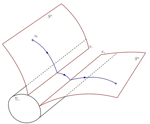
on which the extremal flow is smooth in section1.2.2. The stratum S1 of
codimen-sion one is actually the global stable manifold to a normally hyperbolic submanifold for the regularized vector field contained in Σ. The stratum of codimension two is the singular set Σ´. Indeed, the regularized dynamics, in this region is actually
normally hyperbolic to a submanifold of N in Σ´, and on N the dynamics is
triv-ial: This allows us to conclude regarding the regularity of the strata and of the flow. Furthermore, we prove the continuity of this flow.
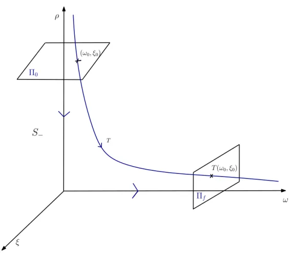
Then, in 1.2.3 we study the transition from a stratum to another one, giving the precise type of singularity occurring: The associated Poincaré mapping turns out to be in the log-exp category. To be able to compute the transition, we use a normal form for our regularized system. We begin by computing formally the normal form: We generalize a theorem of Takens to prove that it is given by a power series in resonant monomials (ie, monomials commuting with the linear part of the vector field). Then, one can use a generalization of the celebrated theorem from Borel to realize this formal series by a smooth function. Once the normal form is obtained, the desired regularity for the transition is achieved by a particular type of blow up. Singularities are of type "d ln d", where d here represents the distance to the stable stratum S1 previously mentioned.
The last section of this chapter is devoted to applications to mechanical sys-tems, and more precisely to the orbit transfer problem. The goal is to make a transfer from an initial orbit to a final one as fast as possible with a bounded con-trol. These problems have a special structure: The distribution pF1, F2q actually
commutes. This implies a special type of switchings called π-singularities: Instant rotations of angle π of the control. The switching function actually verifies an order two linear differential equation, and using a comparison "à la Sturm", we control the number of switchings occurring during a transfer by giving an upper bound linked with the distance to collisions.
Chapter II: Singularities of minimum time
control-affine systems
The last chapter left open the question of the behavior and regularity of the ex-tremal flow around ΣzΣ´. This singularities cannot happen for systems coming
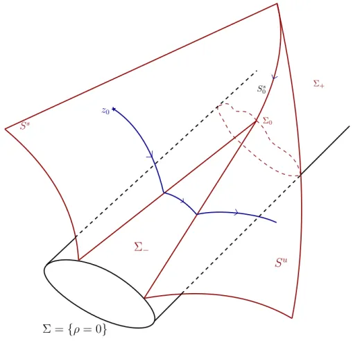
from Newton’s 2nd Law, as shown in section 1.2.4. We provide a complete pic-ture of the behavior of the minimum time extremal flow for generic double input control-affine systems, when the control evolves in a ball. More precisely, the sta-ble and unstasta-ble strata of the previous chapter end up merging, at a nilpotent equilibrium in Σ for the regularized system. Hence, the analysis of the switchings at this point required higher order tools. In section 2.2, we have made a effort to give a reunification of the three types of singularities occurring in Σ: A family of dynamical systems with a parameter is given, the bifurcation between the three cases occurring when the parameter α in (2.2.3) crosses zero.
locus, and dressing a comparison with the single input case. We also have a discussion on the differences between our configuration and the case where the control set is polyhedral. Our singularities can à priori be compared to double switchings in their cases, but it cannot be treated the same way as in [48], for instance. Basically, a bang extremal remains outside the singular locus, and its associated control is smooth. A concatenation of bang extremal is called bang-bang. In chapter I, extremals were either bang or bang-bang, though singular extremals - extremals lying inside Σ - exist in the other cases. The singular flow is smooth, and this chapter also answers the question of the existence of bang-singular connexions. We first deal with the easiest case: Σ`, where the regularized
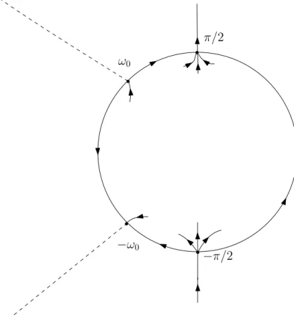
system presents no equilibrium in Σ, implying no switching occurs whatsoever, this can be proved through a simple exponential estimation. Then we tackle the problem of the merging stable and unstable manifold and what happens at the bifurcation. The nilpotent equilibrium is studied through a quasi-homogeneous blow up introduced by Dumortier twenty five years ago in [27]. Successive usual (spherical) blown-ups can be applied to this kind of problems, but there is no guarantee that the desingularization will be successful, it is highly more technical and a difficulty is to go back to the original problem. By finding the right weight when blowing up, most of the time applying this process one time is enough. Once the desingularization achieved, the blown up point turns into a 2-sphere with five new equilibria. The process was successful since they all turn out to be hyperbolic or semi hyperbolic. We take advantage of working in dimension two: There exists a great amount of powerful results for dynamical systems in the plane. We use freely the Poincaré-Bendixson theorem to connect the stable and unstable manifolds from every equilibria in the hemisphere. To that end, one must exclude the existence of periodic trajectory, which we do by considering a well chosen domain, transverse to the vector field and use Stokes theorem to conclude. The existence of a stable direction coming from outside the sphere proves, via an estimation on the initial time, that there exists an extremal going to the singular locus in the nilpotent case (Σ0, below). Regarding the switching on the associated extremal control, there are
two alternatives depending on the sign of the Poisson brackets of the lift of F1 and
F2, H12. The control can be continuous or presents a π-singularity. Then, a similar
analysis of the one in chapter I can be led to build a stratification on which the flow is smooth too. Finally, an informal commentary is made: Through the phase portrait, one can see that the whole situation is contained in this nilpotent case. We end this chapter by providing an example of a non-mechanical control-affine system with the kind of trajectory exhibited in theorem 2.2.
Chapter III: Sufficient conditions for
optimality of minimum time control-affine
systems
Existence and uniqueness for the flow given by the Maximum Principle is of im-portance in optimal control: Provided an optimal trajectory exists, it has to be the extremal. Even though global existence theorems exist, as for instance, Filippov’s [24], it is most of the time difficult to satisfy its their hypothesis without very strong assumptions on the control system. For orbit transfers for instance, it can be applied provided the transfer remains in a compact domain, see [23].
In general, a more reasonable approach is the local viewpoint. The question becomes: Until what time, or point, does a trajectory remain optimal among all nearby admissible trajectories (by an admissible trajectory we mean a solution of the control system for some control u P L8
pr0, tfsq). This particular time is called
a conjugate time, and the associated point is a conjugate point. These concepts are defined by verticality moments of the solutions of the variational equation. That means their definition requires at least a C2 regularity for the Hamiltonian.
In section 3.1, we recall the classical smooth theory of conjugate points, and a local optimality theorem for smooth optimal control systems.
In our case, Hmax is only continuous, and its flow is regular on a
stratifica-tion. We make a comparison with the situation obtained when the control lies in a polyhedron and the results obtained in that case, using, in general, a second order variation for a finite dimensional sub-system. In the next section, we state our result on local optimality among all nearby admissible C0-curves for extremal
trajectories satisfying a disconjugacy condition on the smooth stratum. This con-dition can easily be checked numerically. We prove this result in section3.3, using symplectic methods. The idea is the following: If every curves in the neighbor-hood of the reference extremal trajectory can be uniquely lifted to the cotangent bundle, then one can use the Poincaré-Cartan form pdx ´ Hdt to compare their cost with the reference one. Indeed, it is the natural tool from the definition of the pseudo-Hamiltonian. In the minimum time case, one can use the Liouville form
λ “ pdx. We start by building a Lagrangian manifold L, that is a perturbation of T˚
¯
x0M , so that the intersection with the strata S1 is a smooth submanifold. The
canonical projection
is one to one on the image of the graph submanifold by the flow, ie, on tpt, etHmaxpL X S1qq, t P r0, tfszt¯tuu
where ¯t is the switching time. We can then lift all the nearby admissible curves.
The last step to compare their final time consists in proving the Liouville form is exact, this conducts to the local optimality result.
The last section,3.4, of this chapter is devoted to the proof of the regularity of the field of extremals. This implies the regularity of a upper bound to the value function: we obtain a minimum time depending piecewise smoothly of the end point under assumptions similar to the ones in theorem3.2.
Chapter IV: Non-integrability of the minimum
time Kepler problem
This last chapter is dedicated to study the effect of minimum time singularities on the Liouville integrability in the context of the Kepler problem: One body submitted to the gravitational attraction of a fixed center of mass. The chapter opens on a brief review on Hamiltonian systems, integrability and Galois theory for linear differential equations. The Kepler problem is integrable, and as such, the Liouville-Arnold theorem applies and the phase space is foliated in stable tori, on which the motion is quasi-periodic: The angular coordinates on each torus evolves linearly with time. The aim of this chapter is to prove this structure is destroyed by controlling this problem while minimizing the final time. The Hamiltonian of the minimum time Kepler problem is given by:
Hmax“ maxu tH0` u1H1 ` u2H2u
where is Hi being the canonical lift of the fields Fi and H0 is the lifted Kepler
dynamics, which remains integrable.
Applications of the Galois differential theory methods are rare in the context of optimal control. We give a proof of non-integrability here in the class of meromor-phic functions. We describe Ziglin’s Lemma, but Poincaré already noticed that fact: The first integrals of an Hamiltonian system generate first integrals of its linear part. This translates, through the celebrated Moralès-Ramis theorem, in terms of the Galois group of the variational equation. It is, by analogy with the classical theory, defined as the group of differential automorphisms which preserve the base field. These are algebraic Lie groups and when the system is integrable,
these groups are virtually Abelian: The connected component of the identity has to be Abelian. Another characterization of integrability have been given earlier by Ziglin, through the study of the monodromy group. It is obtained by the action of Π1, the fundamental group, on the solutions by analytic continuation, and is
included in the differential Galois group G of the linearized equation. It is actually dense in G for the Zariski topology. This fact will allow us to upgrade our non-integrability result from the class or rational functions to the class of meromorphic ones.
The first step, and it is one of the difficulties this theory, is to find a solution of the initial (non-linear) differential equation. Most of the time, this is achieved by considering a stable submanifold on which the dynamics is simpler, and often, even integrable. This constitutes a weakness of the theory, according to Ramis, because a system which is very far from integrability does not possess this kind of object. We find a stable surface and an independent first integral on it, which turns out to be a first integral of the Kepler motion with a constant force added. With the choice of our stable surface, our particular solution is the lift of a collision trajectory. We then give a computation of the reduced variational equation is given, keeping only the normal variations to our stable surface. We eventually write a scalar equation from the vectorial one, whose Galois group is contained in
G. The solutions have the form of a product in which one term is a primitive of
the hypergeometric Gaussian function. The Galois group of such functions is thus included in G, and they were classified by Kimura in his paper [36]. Given our parameters, it implies that the Galois group is not even solvable.
Notations.
– Smooth will mean of class C8.– M is a 4-dimensional smooth manifold, Ck
pM q the set of smooth real valued functions on M
– Let F0, F1 and F2 be smooth vector fields on M .
– Let T M and T˚M be respectively the tangent and cotangent bundles of M ,
and π : T˚M Ñ M be the canonical projection.
– Let |v| be the standard Euclidean norm of a vector v P Rn.
– Let r¨, ¨s be the standard Lie bracket of vector fields on manifolds. For two vector fields Fi, Fj we denote their Lie bracket by Fij “ rFi, Fjs.
– For a function H : T˚M Ñ R, we denote X
H the associated Hamiltonian
vector field.
– Similarly, let t¨, ¨u be the standard Poisson bracket on T˚M : In Darboux
coordinates px, pq, tf, gu “ Bf Bx Bg Bp ´ Bg Bx Bf
Bp. For two smooth Hamiltonians Hi
on T˚M , we denote their Poisson bracket by H
ij :“ tHi, Hju, so that if z
is a Hamiltonian trajectory of H, dtdf pzptqq “ tH, f upzptqq. More generally, Hi,i1...,in :“ tHi, Hi1...inu.
– For f P C8
pT˚M q, let ad f : C8
pT˚M q Ñ C8
pT˚M q, with ad f pgq “ tf, gu.
– For an normally hyperbolic equilibrium point z P M , let Ws
pzq (respectively
Wu
pzq) be its stable (respectively unstable) manifold. – Let J :“ˆ 0 1
´1 0 ˙
Singularities of minimum time
control for mechanical systems
We prove the extremal flow of minimum time mechanical systems is piecewise smooth, and smooth on a stratification. There is at most one switching in a neigh-borhood of the singular locus. We give the type of singularities of the transition map between the strata by proving it belongs to the log-exp category. The mini-mum time two and restricted three body problems are studied as an application, and we give a upper bound on the number of switchings in that case.
1.1
Quick introduction to geometric control
& necessary conditions for optimality
In this first section we introduce some of the important notions, tools and main classical result of geometric control theory, that will be of use throughout this thesis.1.1.1
Controllability
Let M be a n-dimensional smooth connected manifold (the state space), and U be an arbitrary set of Rm (the control space). A control system is given by a family
of vector fields f : M ˆ U Ñ T M . This gives us a family of dynamical systems 9
x “ f px, uq (1.1.1)
If one allows the parameter u to change at each time t, we get a classical con-trol problem. Under suitable hypotheses, namely, smoothness of f for instance, by Carathéodory’s theorem, for any control u P U , system (1.1.1) has a unique solution. For a control u P U :“ L8pr0, t
fs, U q, and x0 P M denote xpt, x0, uq the
solution of (1.1.1) with xp0, x0, uq “ x0, or just xptq when there is no ambiguity.
We call U the set of admissible controls. Define the endpoint mapping
Ex0 : u P L
8
pr0, tfs, U q ÞÑ xptf, x0, uq P M.
There are several notions of controllability for a control system. Let us first define the attainable set.
Definition 1.1 (Attainable set)
Let x0 P M , t P R, the attainable set from x0 at a time t is defined by Ax0ptq :“
txpt, x0, uq, u P U u. The attainable set from x0 is Ax0 “ YtPR`Ax0ptq.
We say a control system is controllable from x0 if Ax0 “ M . So the system is
controllable from x0 if the endpoint map Ex0 is onto. It is controllable if this holds
for any x0 P M . We will be interested mainly in control-affine systems, meaning,
systems of the form 9 x “ F0pxq ` m ÿ i“1 uiFipxq, uptq P U (Aff )
For instance, every controlled mechanical system (see 1.1.4 below) is modeled by affine control systems. They can also be seen as a generalization of sub-Riemannian
systems (linear on the control), with a drift added. On a sub-Riemannian system 9
x “ řmi“1uiFipxq, the state cannot only have tangent directions along the Fi’s
but also their Lie brackets (think of the classical example of parking a car): The bracket generating condition
LiepF1, . . . , Fmqpxq “ TxM
for all x P M is sufficient to ensure controllability under suitable hypothesis on the control set U (namely, that its convex hull contains a small ball around 0 P Rm). This result is known as the Chow-Rashevskii theorem. One can intuitively understand that it is not the case in control-affine systems since the drift can be too strong with respect to the control, and thus forbid controllability. There has been a great amount of results on controllability for affine control systems, see for instance Sussman’s conditions or [35]. When the drift is reasonable, ie, does not take the system to infinity, one can imagine that controllability can be achieved. We recall a precise result below, a vector field is called recurrent if its flow has a dense subset of recurrent points. In the systems we are interested in (namely systems from space mechanics), the drift has a chance to be recurrent, and we have:
Theorem 1.1
Consider an control-affine system pAffq. If
(i) F0 is recurrent
(ii) the convex hull fo U contains a neighborhood of 0. (iii) LiexpF0, F1, . . . , Fmq “ TxM for all x P M
then, the system is controllable.
This is a consequence of the orbit theorem, [35]. The bracket generating property is fundamental, and in what follows we will use the following notation for the Lie brackets involved in control-affine problems: rFi, Fjs :“ Fij, and iterating
rFk, Fijs “ Fkij and so on. The same notation will be used for the Poisson brackets:
1.1.2
Geometric optimal control
We would like to control our dynamical system minimizing a criterion, along the trajectories. This criterion will be an integral cost, leading to the following prob-lem: $ ’ ’ & ’ ’ % 9 x “ f px, uq, uptq P U, t P r0, tfs, xp0q “ x0, xptfq “ xf, Cpuq “ ştf 0 ϕpxptq, uptqqdt Ñ min . (1.1.2)
where ϕ : M ˆU Ñ R is a smooth (or continuous) function. In order to understand the mechanisms of the classical necessary conditions for optimality, let us introduce the extended system
$ ’ ’ ’ ’ & ’ ’ ’ ’ % 9 x “ f px, uq, uptq P U, t P r0, tfs, 9 y “ ϕpx, uq, xp0q “ x0, xptfq “ xf,
yp0q “ 0, yptfq “ Cpuq.
(1.1.3)
and the extended end-point map ˜
Ex0 : u P L
8
pr0, tfs, U q ÞÑ pxptf, x0, uq, yptf, x0, uqq P M.
If a control u is optimal, then ˜Ex0puq P B ˜Apx0,0q (with obvious notation) and if the
control set U is open, one can find Lagrange multipliers pP, P0
q P Rnˆ R such that
P.dEx0puq “ ´P
0.dCpuq. This couple of Lagrange multipliers are linked with the
adjoint state in the Hamiltonian formalism given by Pontrjagin to optimal control problems in the late 60’s.
Definition 1.2 (Pseudo-Hamiltonian)
The pseudo-Hamiltonian of system (1.1.2) is defined by Hpx, p, p0, uq “ xp, f px, uqy ` p0ϕpx, uq,
px, pq P T˚M , u P U , p0 P R.
Being in the boundary of the attainable has the following consequence: Proposition 1.1
If u is an admissible control such that Ex0puq P BAx0ptfq, there exists a Lipschitz curve pptq P T˚
xpt,uq for all t P r0, tfs, such that
d
dtpx, pq “ XHpx, p, uq,
The adjoint state pptfq can be built through picking a normal co-vector to an
approximation cone (Pontrjagin’s approximation cone, see [4]) of the attainable set, and then pull-it back by the flow to obtain the whole curve. Many other proofs exist, mainly based on the so-called needle variations, one can be found in [18] for instance. The Pontrjagin’s Maximum Principle (P.M.P.) can be seen as a consequence of this proposition - applied to the extended system - and for free final time, can be stated as follows (see [4] or [51] for the historical paper).
Theorem 1.2 (P.M.P.)
If px, uq is an optimal pair for system (1.1.2), there exists a Lipschitz function pptq P T˚
xptqM , t P r0, tfs, a constant p0 ď 0, ppptq, p0q ‰ 0, such that, for almost
all t,
(i) px, pq is a solution of the Hamiltonian system associated with Hp¨, ¨, uptqq:
9
x “ BH
Bp px, p, uq, p “ ´9 BH
Bxpx, p, uq,
(ii) Hpxptq, pptq, uptqq “ maxvPUHpxptq, pptq, vq,
(iii) Hpxptq, pptq, uptqq “ 0.
The adjoint state can be thought of as a Lagrange multiplier, and actually, up to multiplication with a scalar, we have ppptfq, p0q “ pP, P0q. Integral curves
px, pq of H satisfying piiq and piiiq are called extremals. Their projections on M are extremal trajectories. As in classical Hamiltonian dynamics, and as consequence of the maximization condition, the pseudo-Hamiltonian evaluated along an extremal px, p, uq is constant. Moreover, if the final time is free then this constant is zero. Definition 1.3
The pair pp, p0q is defined up to multiplication by a non-zero scalar. When p0 is
non-zero, we are in the normal case, and one usually renormalize to p0 “ ´1 or
´12. If p0 “ 0, the extremal is called abnormal.
Abnormal trajectories are one of the main difficulties in optimal control: it can be much harder to prove their optimality. The results of chapter I and II of this thesis apply to normal as well as abnormal extremals, as opposed to the ones in chapter III. There exist many versions of the the P.M.P., with fixed final time, for Bolza costs, and so on. For orbit transfer problems, it is convenient to work with boundaries which are not points, but submanifolds, namely, N0,
Nf Ă M . The same result holds with transversality conditions on the adjoint state:
pp0qKTx0N0, pptfqKTxfNf. The maximization condition allows us to calculate the
optimal control, besides, if the maximum is in the interior of the set U , we have
BH
Bupx, p, uq “ 0. This works well for quadratic cost (energy minimization), however
in this whole thesis, we will not be that lucky and the Hamiltonian will reach its maximum on BU (at least outside of the singularities).
Remark 1.1
Setting Hmaxpx, pq “ max
uPUHpx, p, uq, when well defined, allows one to work with a
true autonomous Hamiltonian system, in the sense that it does not depend on the
control. If Hmax is regular enough (for instance, C2 is enough), then extremals are just solutions of the differential equation given by XHmax.
As for time optimal problems, one just has to take ϕ ” 1, but then p0 has no influence on the integral curves, and we can just work with the pseudo-Hamiltonian
Hpx, p, uq “ xp, f px, uqy, with the condition Hpxptq, pptq, uptqq ě 0, and pptq ‰ 0
for a.e. t. Normal extremal correspond to the H ą 0 case, and abnormal ones to
H “ 0. In this chapter, we are mainly interested in the minimum time control of
mechanical systems, namely, systems of the form :
q ` ∇V pqq “ u, (1.1.4)
V : O Ñ R, a smooth function defined on O an open subset of Rn. A mechanical
system is in particular a control affine system
9 x “ F0pxq ` m ÿ i“1 uiFipxq,
with x “ pq, vq, v “ 9q, F0pxq “ v.BqB ´ ∇V pqq.BvB and the vector field supporting
the control, in Cartesian coordinates are Fipxq “ BvB
i. Their pseudo-Hamiltonian
is affine on the control as well with Hpx, p, uq “ H0px, pq `
řm
i“1uiHipx, pq with
Hipx, pq “ xp, Fipxqy. We will consider control bounded in an closed Euclidean ball
U “ Bp0, εq. In the next chapter, we will make a comparison with the case where
the control lies in a polyhedron instead of a ball. Since BH
Bupx, p, uq is everywhere
non zero (except when all the Hi are vanishing), maximizing over all admissible
value of u in the ball, we end up maximizing over its boundary: the sphere. We just proved
Proposition 1.2
The maximal Hamiltonian for minimum time affine control systems is
Hmaxpx, pq “ H0px, pq ` ε
dm ÿ
i“1
Hipx, pq2.
Furthermore, the dynamical feedback on the control gives u “ ε pH1, . . . , Hmq
}pH1, . . . , Hmq}
which belongs to the m-sphere.
Clearly, our maximized Hamiltonian is only continuous, and irregularities of the dynamics occur when all the Hi are vanishing. In the next section, we will be
interested in the behavior of the extremal flow and in the singularities of time minimization, thus, the parameter ε will not have any influence, and we will fix it to ε “ 1. Let us see examples of some of the systems we will tackle.
Example 1.1
The controlled Kepler problem :q ` }q}q3 “ u (}.} denotes the Euclidean norm) in the plane models the motion of a spacecraft attracted by a fixed center. The control u is the thrust of its engine. Thus the maximized Hamiltonian is Hmaxpx, pq “
pq.v ´ pv.}q}q3 ` εap2v1 ` p
2 v2.
Example 1.2
In the controlled planar restricted elliptic three body problem (RE3BP), the third body of negligible mass (a spacecraft or a satellite) is subjected to the attraction of two bodies (positions q1 and q2) in elliptic motion around their center of mass (Keplerian motion). The controlled dynamics is
:
q ` ∇Vµpt, qq “ u, (1.1.5)
with Vµpt, qq “ |q´q1´µ1ptq| `
µ
|q´q2ptq|, the non-autonomous potential. Here, µ denotes the ratio of the masses of the two primaries. We end up with a non autonomous maximized Hamiltonian Hmax
pt, x, pq “ pq.v ´ pv.∇Vµpt, qq ` εap2v1 ` p
2
v2. The P.M.P. holds in that case, see [51].
Both of those examples are affine control problems with double input control (meaning, control vector of dimension 2).
1.2
Singularities of minimum time control
for mechanical systems
We are interested in the optimal time control of affine control systems, more pre-cisely, systems of the form
9
x “ F0pxq ` u1F1pxq ` u2F2pxq,
where the control u “ pu1, u2q is contained in some Euclidean ball and all
vec-tor fields are smooth, in a specific case detailed below, that contains mechanical systems. We also aim at developing a general theory and applying it to space mechanics, namely, to the controlled Kepler and restricted circular three-body problems. In this configuration, the controlled spacecraft (a satellite for instance) is under the influence of two primaries in circular motion. The mass of the satel-lite is supposed negligible with respect to the mass of the two primaries and the dynamics is
:
q ` ∇Vµpqq ´ 2J 9q “ u
where Vµ is the gravitational potential described in example 1.2, and fits our
generic hypothesis (A) given in section 1.2.1. The control u here is the thrust of the engine. See [50] and [6] for more details on the restricted 3-body problem. In [20], the nilpotent case has been extensively treated and the averaged problem is considered. See also [15], where geodesic convexity is proved for the averaged system in the case µ “ 0 (Kepler). Here we will be interested in the original (as opposed to averaged) system. In this matter, the recent work [22] proved the non integrability of the extremal system in the Kepler case, and in [19], the
L1 minimization of the control is studied, and necessary and sufficient conditions for optimality are given. Recently, sufficient conditions for optimality have been also proved in [3] for a minimum time affine control system in a slightly different context. For the sake of simplicity, we carry out the arguments in a 4-dimensional manifold - which is the most relevant for our applications - but the method and result of section 1.2.2 can be adapted to a 2dimensional manifold with an m-dimensional affine control.
In section 1.2.1, we start by recalling some classical results of geometric op-timal control, with a particular emphasis on the Pontrjagin Maximum Principle, which reduces the problem to the study of a singular Hamiltonian system. The singularities of this system are related to the discontinuities of the optimal con-trol u, also called switch. We study the local structure of the Hamiltonian flow