Contingent Loan Repayment in the Philippines

D

OCUMENT DE

T

RAVAIL

DT/2002/14

Contingent Loan Repayment in the

Philippines

Marcel FAFCHAMPS

Flore GUBERT

CONTINGENT LOAN REPAYMENT IN THE PHILIPPINES. Marcel Fafchamps

(Centre for the Studies of African Economies, University of Oxford) marcel.fafchamps@economics.ox.ac.uk

and Flore Gubert

(DIAL – Unité de Recherche CIPRE de l’IRD) gubert@dial.prd.fr

Document de travail DIAL / Unité de Recherche CIPRE

November 2002

RESUME

Cet article examine les pratiques d’un échantillon de ménages ruraux en matière de remboursement de crédit, à partir de données collectées aux Philippines. L’analyse économétrique montre que les chocs subis par l’emprunteur et son créancier exercent une influence significative sur la durée de l’emprunt, mais qu’ils sont sans effet sur le montant du remboursement ni sur la probabilité que l’emprunteur bénéficie d’une remise de dette. Par ailleurs, les emprunteurs ayant subi les désagréments d’un choc tendent à rembourser leurs prêts en travail plutôt qu’en argent. Les intérêts versés sont souvent moindres que les intérêts dus ex post, mais ne sont pas directement influencés par les variables de choc. Enfin, les phénomènes d’asservissement des emprunteurs ou de surendettement ne sont pas observés dans la zone d’étude.

ABSTRACT

This paper examines credit repayment among rural Filipino households , using survey data collected in four villages in the Cordillera mountains of northern Philippines between July, 1994 and March, 1995. We find that the timing of loan repayment depends on shocks affecting lender and borrower but amounts repaid and debt forgiveness do not. Borrowers occasionally repay debt in labor when faced with a bad shock. Contractual interest charges often are reduced ex post but reductions do not depend on shocks except through the timing of repayment. We find no evidence of loan roll-over, debt peonage, or labor bonding.

Table des matières

1. Introduction ……….4

2. Conceptual framework ………..………..……….………..5

3. The data ………..8

4. Testing contingent repayment ……….10

4.1. Timing ……….12 4.2. Amount paid ………12 4.3. Form of repayment ……….………13 4.4. Debt forgiveness ……….14 4.5. Future lending ……….15 5. Conclusion ………..16 References

Liste des tableaux

Table 2. New loans ………..………21

Table 3. Participation in informal credit ………22

Table 4. Reason for receiving a loan ………23

Table 5. Propensity to repay ………24

Table 6 Propensity to repay controlling for individual effects ………..………..25

Table 7. Total amount repaid ………26

Table 8. Repayment in labor ………..……….28

Table 9. Debt forgiveness ………..……….29

Table 10. Expectations of future lending ……….30

1 . I N T R O D U C T I O N

Risk is part of life. The way people and firms deal with risk therefore affects many aspects of economic activity. This is true everywhere, but is particularly marked in poor rural economies where the magnitude of risk is larger and individual capacity to deal with risk is less Fafchamps 1999b). Economic agents have devised a variety of strategies to cope with risk: transfers, precautionary savings, risk pooling, labor market participation, etc. (e.g. Townsend 1994, Morduch 1995). We focus here on one of these strategies: borrowing.

It is increasingly recognized that loans play an important role in the way people deal with risk (e.g. Rosenzweig 1988, Imai 2000). There are conceptually two ways by which loans can be used for risk purposes. First, individuals or firms can take up new loans when they have been hit by a shock. Fafchamps and Lund (2002), for instance, show that rural Filipino households borrow from friends and relatives when affected by income or health shocks. In anticipation of this, individuals or firms may set up networks of people who can help them in times of trouble (Banerjee and Munshi, 1999). An alternative way of achieving the same outcome is for economic agents to open a line of credit beforehand. Overdraft facilities are examples of such lines of credit. Fafchamps, Pender and Robinson (1995) and Fafchamps, Biggs, Conning and Srivastava (1994) show that overdraft finance is the dominant form of enterprise credit in Sub-Saharan Africa and that manufacturing firms rely on it to deal with changes in liquidity requirements.

There is also a second way by which credit can be used to cope with risk: contingent repayment. Udry (1994), for instance, demonstrates that the repayment of informal loans is contingent upon shocks affecting lender and borrower. In a survey of manufacturing firms reported by Fafchamps et al. (1995), firms were asked how they deal with liquidity crises. One of the most often cited response was to delay payment to suppliers. Some firms even went as far as delaying payment to employees, but this was seen as a last resort action.

Contingent loan repayment has been discussed extensively in the literature -- most notably in the literature on sovereign debt where debt repayment is often renegotiated (e.g. Eaton and Gersovitz, 1981, Eaton, Gersovitz and Stiglitz 1986, Kletzer 1984, Grossman and Van Huyck 1988). What remains unclear, however, is how contingent repayment is organized. Is it through delay in repayment (debt rescheduling), reduction in repayment (partial or complete debt forgiveness), or issuance of new debt (debt roll-over)? Under what circumstances does payment in kind or in labor replace payment in cash? Do lenders take advantage of borrowers' difficulties to force them into a debt trap, sometimes called debt peonage or labor bonding in the literature (e.g. de Janvry 1981, Bardhan 1984, Srinivasan 1989, Genicot 2002)?

These issues are the focus of this paper. We examine debt repayment practices among a sample of rural Filipino households. The data were collected from 200 rural households during three visits covering a 9 months period. Detailed information relative to all loans and loan repayment was collected. Data were also collected on shocks affecting respondents and their lenders.

As Udry (1994), we find that loan repayment depends on shocks affecting both lender and borrower. But the form contingent repayment takes is not what is usually assumed, e.g., a reduction in the amount repaid. Our results indicate instead that debt rescheduling is the dominant form of contingency: borrowers delay repayment when they are hit by a shock, and accelerate repayment when the lender is hit by a shock. These results are consistent with Udry (1990)'s description of

informal lending in Northern Nigeria. In contrast, when the debt is paid, the difference between the amount contracted and the amount repaid is in general small and need not depend on shocks. Debt roll-over is uncommon. Although some loans are made at usurious interest rates, we find no evidence of debt trap. There is, however, some evidence that debtors unable to repay in cash volunteer their labor as repayment. As far as we can judge, this practice does not seem to be associated with labor bonding in the survey area.

The paper is organized as follow. We begin in Section 2 by providing a conceptual framework for contingent loan repayment. We examine the conditions under which debt peonage or labor bonding are likely to arise. Forms of contingent repayment are contrasted with the help of a simple model. We show that debts based on the continued voluntary participation in long-term relationships are more likely to resort to debt rescheduling rather than debt roll-over. In a perfect risk sharing equilibrium, gifts and transfers should be made to help pay off debts. Section 3 discusses the data collection methodology. A simple test of contingent repayment is presented in Section 4. A more detailed analysis of the forms of contingent repayment appears in Section 5.

2 . C O N C E P T U A L F R A M E W O R K

To focus the attention on loan repayment, we consider a two-agent debt repayment game. Throughout, borrower and lender are denoted with the superscripts b and l, respectively. The model is recursive. Assets are ignored. The stock of debt at the beginning of period t is denoted Dt. During

period t, borrower and lender each incur an income shock _si i

{ }

t, = , .

1

Repayment is written Rt. The instantaneous utility of the borrower is written Ub(cbt) with

R s y R c c t bt t b t b t b

t = − = + − . The utility of the lender is Ul(clt) with c y slt Rt l

t l

t = + + . In both cases,

yi denotes the expected income of agent i. For simplicity, we assume that incomes are iid. Negative consumption is not feasible, i.e., y sbt Rt

b

t+ ≥ . This means that the borrower cannot repay in period t

more than his current income.

In each period, borrower and lender renegotiate debt repayment. We begin by assuming that the lender has all the bargaining power. We revisit this assumption later in this section. Repayment by the borrower is voluntary in the sense that agreeing to the lender's conditions must leave the borrower better off than breaking the relationship. We call breaking the relationship a default. We assume that, in case of default, the lender can credibly inflict legal and extra- legal penalties denoted

Pt 0. In general, these penalties depend on the stock of debt so that Pt = P(Dt+1) with P 0. Legal

penalties primarily take the form of court action. Examples of extra- legal penalties include recourse to 'loan enforcers' and exclusion from other social intercourse (Spagnolo 1995). If penalties are not credible, Pt=0 (Fafchamps 1996).

With these assumptions, the model takes the form of an agent-principal model: ) ( ) ( max _{, 1} 1 + + + + + l t l t l t l t l D Rt t U y s R β EV D subject to (2.1) t D P EV s y U D EV R s y U b b _{b t} t b t b t b b t b t b t b( + − )+β ( +1) ≥ ( + )+β (0)− ( +1) ∀

1 _{Consumption shocks such as sickness that requires health expenditures can be treated as utility shocks as in} (e.g. Mace 1991, Cochrane 1991)

t R s y bt t b t + ≥ ∀

where the first inequality is the voluntary participation constraint and the second is the feasibility constraint. Parameters are the discount factors of the lender and the borrower, respectively. We assume that the borrower worries about starvation, i.e., lim_c→0U_b(c)=−∞. In this case, the second constraint is superfluous. Since the borrower's utility is monotonically decreasing in Rt and the

penalty is monotonically non-decreasing in Dt, it is always in the lender's interest to choose Rt and

Dt+1 such that the voluntary repayment constraint is binding.

If P(D)=0 for all D, repayment is still possible but only if the lender provides insurance. Bulow and Rogoff (1989b) derive a similar result for sovereign debt. In this context, the optimal debt contract becomes fully contingent and resembles an insurance contract (Grossman and Van Huyck 1988). If the lender is risk neutral, the optimal repayment schedule is such that the borrower's consumption is constant. The expected gain to the borrower is an increasing function of the borrower's willingness to pay for insurance, that is, of his risk aversion. Only if the borrower is risk neutral is expected repayment 0 (Fafchamps, 1999a). If the lender is risk averse, the optimal debt contract resembles mutual insurance: when the lender receives a negative shock, repayment is higher and debt falls faster (Ligon, Thomas and Worrall 2000).

When computing EV_l(D_t+1), the lender takes into account the possibility of future default. But in the model 2.1, it is never in the lender's interest to force the borrower into actual default. This is because we have implicitly assumed that the lender does not benefit from imposing the penalty. In this case, the lender's payoff is highest if he continues extracting regular debt repayment Rt from the

borrower. This situation is what some have described as debt peonage: the borrower is 'prisoner' of the lender and obligated to permanently repay a never-extinguished debt. Note, however, that if

P(D) is 0 or close to 0 for all D, the lender must provide insurance to the borrower otherwise

) 0 ( ) ( _{t 1 b} b D EV

EV ₊ < and default occurs. Only if P(D) is high enough can positive payments be extracted in all states of the world (Bulow and Rogoff 1989a).

If the lender directly benefits from imposing the penalty, default eventually occurs. Let Q(Dt) be the

lender's payoff if the penalty is imposed. Suppose that there exists a high enough Dt+1 such that

) ( ) 0 ( ) ( _t+1 < _l + _t+1 l D EV Q D

EV Then it is always in the lender's interest to set Dt+1 such that:

) ( ) 0 ( ) ( _t+1 < _l + _t+1 l D EV Q D EV (2.2)

For any finite P(Dt+1), default is ensured by setting Rt at the highest possible level -- so that

) (y s R U bt t

b t

b + − tends to - . In this case, the voluntary repayment constraint is violated and default

occurs. Labor bonding -- i.e., a defaulting borrower becomes the slave of his lender -- is an example of such situation (Genicot 2002). The lender may also perceive a high utility from punishing the borrower out of anger or spite (Becker and Madrigal 1994).

What the above discussion has made clear is that, without additional restrictions on the relationship between Dt, Rt, and Dt+1, the model instantaneously results in either debt peonage or labor bonding.

This is because the lender has too much power. Restrictions on the relationship between Dt, Rt, and

Dt+1 may come from various sources. Laws regarding usury and admissible contractual penalties for

late payment set a cap on the speed with which the debt can rise. The lending contract may also specify beforehand what fees and interest charges are assessed in case of non-payment. For instance, if the maximum admissible interest rate is rmax, then the lender faces an additional constraint:

) 1 )( ( max 1 D R r D_t+ ≤ _t − _t + (2.3)

If such a constraint is present, it is always in the interest of the lender to set )

1 )(

( max

1 D R r

D_t+ = _t − _t + since this maximizes future repayments. If rmax is high and Dt is large

relative to what the borrower can pay, the nominal debt increases exponentially and eventually exceeds the value of all future payments the borrower can ever make.2 _{When this happens, debt}

peonage or labor bonding again obtain. Societies may seek to prevent this occurrence by forbidding usury.

Competition in the credit market also imposes limits on the speed at which debt can accumulate. If the borrower can borrow from other sources at a rate r < rmax, any attempt by the lender to impose

rmax leads the borrower to borrow Dt elsewhere at rate r to pay off his debt to the lender. This

ensures that the borrower does not incur the default penalty P(Dt). In the perfect competition case, r

is equal to the riskless interest rate plus a risk premium (e.g. Kletzer 1984,Grossman and Van Huyck 1988). As the borrower's debt increases relative to his ability to pay, the risk premium increases as well so that, even in a perfect competitive economy, an unlucky borrower eventually ends up as a debt peon -- not to a particular lender but to the collectivity of lenders. To prevent this occurrence, many societies have bankruptcy laws for corporations. Except for the US, however, most societies do not recognize individual bankruptcy, in which case past debts are never extinguished and debt peonage is legally possible.3 _{In this case, debt is only extinguished by the}

death of the debtor.4

Having clarified the factors that affect the path of debt repayment, we turn to the debt contract proper. For a lender and a borrower to voluntarily enter in a debt contract, they must both benefit from it. For the lender, this means that V_l(D₀)≥V_l(0): lending yields more utility. If the lender is risk neutral, this boils down to:

0 1 ] [R D E _t t t l ≥

∑

The borrower must also agree to the contract. This requires that ) ( ) 0 ( V D₀ V_b ≤ _b (2.5)

where Vb(D ) internalizes the fact that, in some future state of the world, the borrower may want to

default and incur the penalty (Fafchamps 1996). If repayment is too high, the borrower prefers not to borrow. The same occurs if repayment is insufficiently flexible so that default is likely, and if the penalty for default is high. By the same token, a contract with rigid repayment is not attractive to a borrower who faces a lot of income risk. A borrower may nevertheless accept a disadvantageous contract if he is very impatient (e.g., drug addict, compulsive gambler) or if he is on the brink of starvation, so that money today is worth much more than money tomorrow. For this reason, we

2

Examples of this kind of situation can be found in sovereign debt contracts when nominal debt is sold at a discount on secondary markets.

3 _{To our knowledge, the Philippines do not have personal bankruptcy laws.} 4

expect poor people facing a lot of uninsured risk to voluntarily enter in debt cont racts leading to debt peonage or labor bonding.

This rapid overview of contingent debt contracting has taught us a number of lessons. If borrowers are risk averse, debt repayment should be contingent on shocks affecting the borrower. If lenders are risk averse, repayment should be contingent on shocks to lenders as well. If penalties can be inflicted upon defaulting borrowers, free debt contracting leads to permanent indebtedness (debt peonage) or to labor bonding for unlucky borrowers (Fafchamps 2003). Borrowers fall faster into permanent indebtedness if there is little competition between lenders or if there are few legal or customary restrictions on interest rates (prohibition of usury). If penalties for default are low, reversals of financial flows should be observed: fresh money should flow from lenders to borrowers when borrowers are faced with large negative shocks. If penalties are high enough, it is possible to observe unidirectional flows but contingent repayment is still optimal.

These predictions all rest on the assumption that borrower and lender can observe shocks sbt and slt.

If shocks are not observable, lenders cannot condition repayment on sbt . Leaving repayment at the

discretion of the borrower creates moral hazard, since it is in the interest of the borrower to falsely report shocks to abscond from repaying the debt. In this case, rigid repayment may be optimal. Another possibility is to give the borrower some limited discretion regarding the timing of repayment, e.g., to let arrears accumulate up a given ceiling or to allow delays of up to 60 days -- provided the borrower is in 'good standing', that is, has not abused this flexibility in the past. This discretion works like a line of credit or overdraft facility. It can improve upon a rigid repayment schedule by providing limited insurance to the borrower.5

Armed with the conceptual framework, we now examine debt repayment practices among rural households. Our main objective is first to assess whether debt repayment depends on shocks affecting lender and borrower. We then examine what form contingent repayment takes. Do borrowers delay repayment or is the amount repaid affected as well? In what form do they repay the debt? Is there evidence of debt roll-over? We pay special attention to any possible evidence of debt peonage and labor bonding.

3 . T H E D A T A

Having presented the conceptual framework, we now describe the data. A survey was conducted in four villages in the Cordillera mountains of northern Philippines between July, 1994 and March, 1995 (Lund 1996). A random sample of 206 rural household was drawn after taking a census of all households in selected rural districts. These households are dispersed over a wide area; most can only be reached by foot. Three interviews were conducted with each household at three month intervals between July 1994, just after the annual rice harvest, and March 1995, after the new rice crop had been transplanted. The data contain detailed information on debt and shocks.

Data were collected on the characteristics of each household. Respondents were also asked to list all loans taking place within the last three months of each survey round. Great care was taken to collect data on all possible in-kind loan payments, including crops, meals, and labor services. The characteristics of each transaction were recorded.

5

Banks often operate in this manner. They typically combine a loan with an overdraft facility. The loan has a rigid repayment schedule, but the overdraft facility gives the borrower certain discretion in the timing of repayments.

Information was also gathered on a variety of income and consumption shocks, such as crop failure, unemployment, sickness, and funerals. Events, such as sickness, that require the organization of traditional religious ceremonies are included as well. In addition, we collected an aggregate subjective measure based on respondents' own assessment of their financial situation. This measure combines many simultaneous shocks and allows respondents to attach their own weight to particular events.6 _{Responses range from -2 for very good to +2 for very bad. A similar ranking was}

obtained for a large proportion of partners in loan contracts. Data are available on each of 206 households for three survey rounds (see Lund (1996) for details).

Sample households derive most of their income from non- farm activities (Table 1). There are many skilled artisans in this area, and their wood carvings, woven blankets, and rattan baskets supply a growing tourist and export trade. Unearned income -- mostly land rentals -- is not negligible but very unevenly distributed across households, as is often the case with asset income. Although nearly all households operate their own farm, the majority do not produce enough grain to meet annual consumption needs. Sales of crops and livestock account for a minute fraction of total income. Surveyed households are net recipients of gifts and informal loans.

The vast majority of rural credit transactions are composed of consumption loans between relatives and neighbors. Borrowing from formal credit institutions is rare: only 3.8% of loans in the study are from credit cooperatives, banks, or government organizations.7 _{Because these loans are larger,}

however, they account for 19.4% of new loans in value terms. Formal loans are mostly disbursed for production purposes. Store credit and advances from middlemen account for 28.2% of all new loans and another 13% of new loan value. These two categories of loans are likely to have a profit-seeking motive. Together they constitute what, in this paper, we call formal loans.

The remainder, which we call informal loans, take place between people who know each other well. In value terms, loans from relatives represent 72.5% of new borrowing (Table 2). Over 80% percent of informal lending occurs between households in the same village; virtually all others loans are taken from adjacent villages. Borrowers and lenders are well-acquainted: in nearly all cases, they describe each other as relatives or friends and in more than 85% of the cases, respondents were able to provide a complete accounting of the wealth holdings and demographic characteristics of all their loan partners.

Participation in informal le nding is widespread (Table 3). Only three households in the sample of 206 were not involved in any informal credit transactions over the three survey rounds, while 92% of the households borrowed and 61% lent. Over half of the sample households participated in both borrowing and lending. Informal loans are not exchanged on an anonymous basis within a large community or market but rather through a network of personalized relationships. 92% of households have had credit transactions with their current loan partners in the past, and the same proportion expect to transact again in the future. Over half the households have reversed roles with their loan partners: current borrowers have given loans to their lender in the past and current lenders have received loans from borrowers. Obtaining credit in the future may thus be a motivation for extending loans today. Furthermore, repeated interaction seems required to build trust between

6

For example, one respondent whose spouse had been very sick paradoxically ranked herself better during the survey period than during the preceding one. When questioned, the respondent explained that a child got a new job, and that this happy event far outweighed the costs of her husband's sickness.

7

The small percentage of formal sector loans in the study is consistent with other studies of rural credit. Udry (1990) and Udry (1994) finds that only 7% of loans in northern Nigeria are from the formal sector. Rosenzweig (1988) reports that 13% of loans in the ICRISAT dataset are from formal institutions. In a study of informal credit in Asia, Ghate (1992) suggests that up to 1/2 of all loans are informal in Thailand, up to 2/3 are informal in Bangladesh, and over 2/3 are from informal sources in the Philippines.

network partners: during the interviews, many respondents stressed the role of trust building before loans can take place. At prima facie, the model developed in Section 2 is thus well adapted to our study area.

Most informal loans are taken for consumption rather than investment purposes.8

Table 4 shows that the most common reason for borrowing is to meet immediate consumption needs. Only 17.2% of informal loans are used for investment purposes, mostly schooling. This raises the possibility that the primary motivation behind informal loans is to smooth consumption. Some gifts are motivated by the desire to repay for a previous loan. In addition, respondents explicitly reported that 5.9% of the loans were taken so that the borrower could give or lend the money to someone else. The fact that households act as intermediaries in transferring loans from one friend to another indicates that informal credit is not exchanged through a market system but rather through a network of personal contacts. The small proportion of relending nevertheless suggests that loan intermediation is not frictionless.

Informal loans appear quite flexible. None have written contracts, less than 4% specify repayment schedules, and only 0.7% require collateral. Although 18% of the informal loans repaid during the survey period were not repaid in full, and 6% actually earned a negative return, in only one instance did a lender claim that a default had taken place. In the other cases both lenders and borrowers agreed to forgive part of the loan. By the same token, in 10% of all loans the borrower repaid more than the amount owed. Similar evidence has been reported by Udry (1994) and Platteau and Abraham (1987).9 The majority of informal loans, nearly 86%, charge no interest. This feature is shared by most loans between friends and relatives around the world (e.g. Ben-Porath 1980, Zeller, Schrieder , von Braun and Heidhues 1993). For interest-bearing loans, the interest is calculated monthly without compounding. So, a 5% loan of 1000 pesos carries a constant 50 pesos monthly interest charge.

4 . T E S T I N G C O N T I N G E N T R E P A Y M E N T

As discussed in Section 2, current theoretical thinking about informal debt contracts revolves around the concept of contingent repayment. The work of Udry (1994) on Northern Nigeria rural lending is usually cited as evidence for it. Udry's work, however, does not distinguish between various forms of contingency, e.g., delaying repaying vs. partial debt forgiveness. In this section, we test whether contingent repayment occurs and, if so, what form it takes. We examine four dimensions of repayment: timing; amount paid; form; and amount remaining due.

Factors influencing repayment are the amount of the loan still due and shocks affecting borrower and lender. The amount due Dt is decomposed as follows:

∑

Loans from banks and credit cooperatives, in contrast, are given for investment purposes only. Kochar (1997) reports similar restrictions on formal lending in India.

9 _{Given these features, one may wonder whether such transactions should be called loans or something else} entirely, such as quasi-credit as in Platteau and Abraham (1987). What is important for our purpose is that respondents draw a sharp distinction between the two in that the obligation to repay an informal loan is regarded as much stronger than the diffuse obligation to reciprocate a gift. Quasi-credit is formalized in Fafchamps (1999a).

where L is the loan amount given at time 0, r is the monthly interest rate, t is the time elapsed since the loan, Rô is repayment at time ô, and:

) 1 ( 1 0 1 0 rt L R S t t ≡ −

∑

The appeal of equation 4.1 is that it lends itself easily to logarithmic transformation. As is clear from 4.1, Dt can be decomposed into three components: the original loan amount L ; an interest

factor 1+rt, which is 1 for zero- interest loans; and St, the share of the total amount due that remains

to be paid. In our analysis, we enter these three components separately and in log form. If repayment is proportional to Dt without difference across loan size and interest rate, all three terms

should have the same coefficient of unity. A loan is assumed fully repaid if Dt 0; observations with

Dt 0 are thus dropped from the sample.

Regressors for shocks sbt and sltare constructed as follows. Information on shocks affecting the

respondent is available for each of the three survey rounds. Respondents were asked to rank their current situation relative to normal. They were also asked about a variety of specific shocks, such as disease, loss of employment, and death in the family. To reduce measurement error in the subjective ranking variable, we instrument it using specific shock information as well as individual fixed effects and village-time dummies. The instrumenting equation is presented in Appendix A1.

Information was also collected on shocks affecting the other party to the loan contract, whether borrower or lender. This variable takes the form of a ranking from -2 (very good) to +2 (very bad). This ranking, however, is not available for all loan contracts. To avoid losing too many observations, we set missing partner shocks to the median of 0.

To prevent the estimations being affected by omitted variable bias, we include additional controls related to the characteristics of the responding household and its partner(s). The vector of household characteristics includes the age in years of household head, the number of years of schooling completed by household head, a dummy indicating the male household head has craft or carpentry skills, a dummy indicating the head or spouse has a permanent job, the size of the household in adult male equivalents and the value of household wealth evaluated at the start of the survey. Information concerning the transaction partner includes the age in years of household head and the level of income. This latter variable takes the form of a ranking from 1 (poor) to 4 (rich).

Three sets of regressions are computed. We first distinguish whether the respondent is the lender or borrower. If the respondent is a lender, slt is the shock to the respondent while sbt is the shock to

the other party. The reverse is true if the respondent is the borrower. We therefore expect the sign on respondent and partner shocks to switch when the respondent is lender.

When the respondent is a borrower, we further distinguish between informal and formal loans. For memory, formal loans are defined here as all loans from shopkeepers and financial organizations.10

It is fair to assume that these loans are primarily granted for commercial reasons. Because most formal lenders are large organizations or businesses, the information on shocks affecting them is not relevant (as we expect these lenders to be approximately risk neutral) and is consequently missing for nearly all formal loan contracts. For this reason, the vector of regressors entering the formal loan

10

regressions only includes information on borrowers. When lending is part of business, we expect that lenders display less flexibility and insist on timely payment.

Informal loans are all loans among individuals and are generally not granted with a profit motive. In agreement with the model presented in Section 2, we expect contingent repayment to be present in informal loans.

4.1 T i m i n g

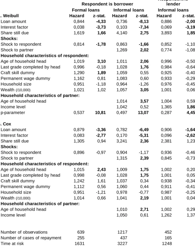
We begin by examining the number of months elapsed between the time at which the loan was granted and the time in which it was repaid. The timing of repayment is analyzed via a duration model. The hazard repayment function describes the borrower's conditional propensity to repay. One way of making repayment contingent on shocks is simply to let the borrower repay late. Results are presented in Table 5. Two estimators are computed: a parametric Weibull duration model, and a semi-parametric Cox model. The Weibull model imposes a parametric functional form on the hazard; the Cox model does not.

When the respondent is the borrower, results by and large conform with expectations: shocks affecting borrowers sbt delay repayment while shocks affecting informal lenders s

l

t speed up

repayment. The magnitude of the effect is broadly similar across the Weibull and Cox models, albeit the borrower shock is not significant for informal loans in the Cox model. When the respondent is the lender, shock variables are never significant.

We find that large loans and loans bearing interest tend to be paid more slowly. This is true for all categories of loans. At the same time, borrowers are more likely to pay when St is large, that is,

when the loan is still due in full. We also find that formal loans are repaid faster than informal ones. The fact that loans bearing interest are repaid more slowly is a priori puzzling: delaying increases the interest charge so that it would be in the borrower's interest to speed up repayment. As we shall see below, interest charges often are renegotiated ex post so that delaying need not carry much penalty. Other results of interest show that certain categories of borrowers (older, better educated and wealthier) tend to repay faster.

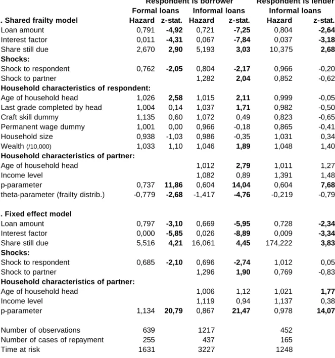
The results presented in Table 5 may be affected by unobservable individual effects. This is particularly true for amount due and interest rate: if unreliable borrowers are also those that accumulate large, interest-bearing debt, the negative effect of loan size and interest charges could be due to an omitted individual effect. To investigate this possibility, we estimate two alternative models: a shared frailty model, and a 'fixed effect' model. The shared frailty model is roughly equivalent to an individual random effect model. We assume a Gamma distribution for frailty. The fixed effect model is estimated by adding individual fixed effects to the Weibull duration model. Results are summarized in Table 6. Controlling for individual unobservables does not affect our earlier results. Loan size and interest charge effects are not driven by unobservables: given a choice, borrowers first repay small, non interest-bearing loans.

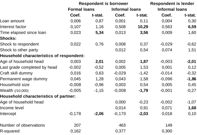
4.2. A m o u n t p a i d

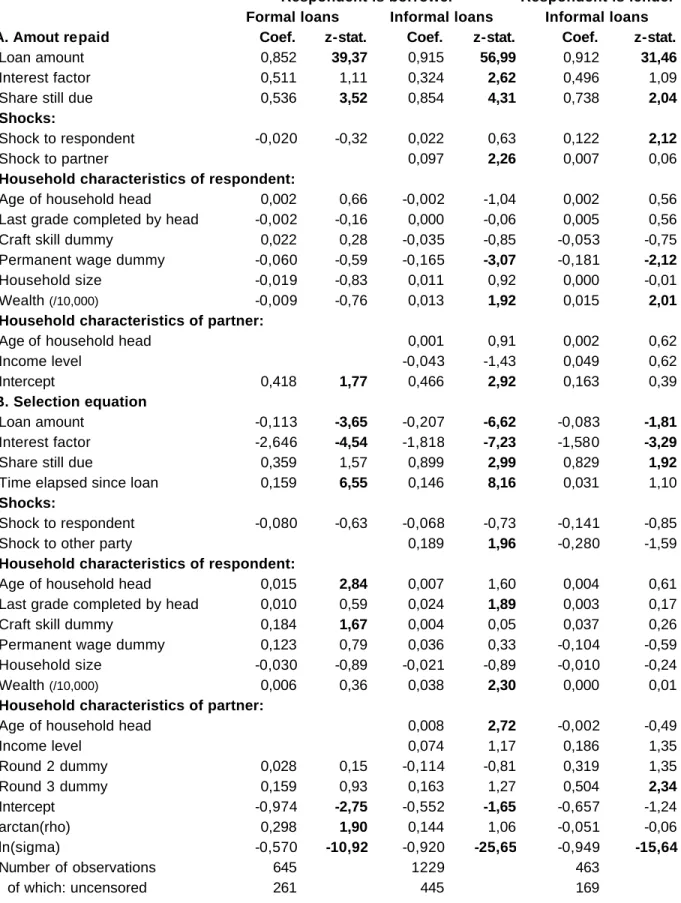
Next we turn to the amount paid conditional on repaying. To this effect, we estimate a maximum likelihood selection model. The regressors entering the amount paid equation are the same as in the duration model. In the selection equation, we control for duration effects by including round

dummies and a regressor measuring the time elapsed between the loan and the beginning of the survey round.11

Results are presented in Table 7. The selection equation simply confirms earlier results. The propensity to repay a loan decreases with loan amount and interest rate; it also responds to shocks affecting lender and borrower, but only for informal loans when the respondent is borrower. In contrast, the amount paid equation contains some surprises. First, we find that shocks to the borrower never have a significant effect on the amount repaid, conditional on repaying. In the informal loan regressions (columns 2 and 3), the regressor even has the wrong sign. The amount paid responds to shocks to the lender in the informal loan regressions, however.

Second, we find that the amount paid is roughly proportional to the loan amount Lt and the share

due St, as could be expected. But in the informal loan regression the coefficient on the interest factor

is significantly smaller than 1, suggesting that interest charges are not paid in full. We also find that the coefficient on Lt is significantly smaller than 1 in all cases, indicating that loan repayment does

not increase proportionally with the size of the loan.

4.3. F o r m o f r e p a y m e n t

Next we turn to the form of repayment. In the area studied, repayment takes essentially two forms: cash and labor. To allow comparison, labor values were imputed by respondents.12

Some 17% of all loan repayments take the form of labor. In all cases except 2, repayment within a specific survey round is either in cash or in labor. We therefore estimate a logit model of whether repayment takes the form of labor or not, conditional on repaying. The determinants are the same as before, except that we include round dummies to capture possible seasonal effects. Time elapsed since the loan was granted is also included to check whether payment in labor is more likely for old unpaid loans, a finding that would support the labor bonding story.

Results are presented in Table 8. The estimator is logit.13 _{Only observations with a repayment are}

used for estimation. The regression therefore captures the probability of repayment in labor, conditional on repayment taking place. For formal loans (column 1), shocks are not significant. In contrast, for informal loans (column 2), shocks to the respondent have the expected sign. Conditional on repayment occurring, a borrower experiencing a bad shock is more likely to repay in labor. The coefficient of partner shock has the right sign but is not significant. The evidence therefore suggests that payment in labor is substituted for cash payment by borrowers in difficulty. We also find that, for formal loans, payment in labor is more likely for large loans but inexistent for formal loans carrying interest. The latter category includes primarily loans from financial institutions that, by definition, are not designed to accept payment in kind. As far as formal loans are concerned, payment in labor concerns primarily shopkeepers. In this case, we have some evidence of labor bonding, i.e., highly indebted individuals providing labor payments. However, we do not find that labor payment increases over time, as would be suggested by the labor bonding model.

11

Both round dummies and time elapsed are non significant in the amount paid equation but jointly significant in the selection equation. They can therefore serve as identifying restrictions.

12

This is a fair question since all loans are stipulated in monetary terms and respondents must have agreed with the lender by how much of the loan is reduced when they work for them. In a few cases when labor value is missing, we impute a value using the median wage rate.

13 _{We also estimated a multinomial logit model with three choices: (1) not paying; (2) repaying in labor; and (3)}

repaying in cash. Identical conclusions obtain. We also estimated a fixed-effect logit model, but the number of remaining observations is too small for inference purposes (i.e., none of the regressors is significant).

A different picture emerges for informal loans. In this case, payment in labor is less likely for large loans. In those cases, payment in labor appears as a friendly way of reciprocating for small financial assistance. When the amount is larger, repayment in cash is expected. Also, payment in labor is less likely for old loans. What this suggests is that borrowers unable to pay on time volunteer their labor, possibly to demonstrate good faith. This explains why payment in labor takes place early on, not later as would be the case for labor bonding.

Taken together, the evidence therefore suggests that labor bonding is not a feature of informal lending although the possibility of labor bonding cannot entirely be ruled out for loans from shopkeepers. This finding is in close agreement with the description of labor bonding and debt peonage made by (Geertz (1963) in neighboring Indonesia: it is a feature of the emerging market economy, not of 'traditional' rural society.

Other results of interest in the informal loan regressions show that the wealth of borrower and lender affect the probability of repayment in labor in opposite direction. Conditional on repayment taking place, repayment in labor is less likely for rich borrowers, while rich lenders are more likely to be repaid in labor.

4.4. Debt forgiveness

So far we have examined actual debt repayment. There remains the possibility that borrowers who face a bad shock are simply dispensed from repaying a loan or from repaying it in full. To examine this possibility, we make use of information collected at the end of the survey. Respondents were asked the amount remaining due on each individual loan. We call the amount the implicit debt and denote it Ù. For 42% of the loans, Ù=0. Other loans have remaining balances. The debt forgiveness ratio φ can then be computed as:

0 3 L D −Ω = φ

where L is the loan principal and D is the amount due as stipulated in the contract -- the 'contractual debt' -- obtained from equation 4.1.

In 13% of the cases, φ is negative: the borrower paid more than was stipulated in the contract. In 63% of the loans, D =Ù so that the contractual debt matches exactly the amount considered due by respondents at the end of round 3. In the remaining 24% of cases, the contractual debt is higher than what respondent thinks has to be paid. In most cases the difference is a small proportion of the principal. But for 10% of the loans, the difference exceeds 50% of the principal. Of course, part of the discrepancy between our estimate of the contractual debt and the amount respondents consider due may be driven by error of measurement: our measure of φ is noisy. This is why we need a statistical approach.

We now investigate whether φ responds to shocks by regressing it on shocks and the three components of D . Regression results are presented in Table 9. Shock variables are not significant in any of the regressions. In the informal loan regressions, one variable dominates the results: the interest factor 1+rt. In two out of three regressions, the time elapsed since the loan was granted is significant as well, suggesting that unpaid loans become 'forgiven' as time passes -- at least in the eyes of respondents. To ensure that these results are not driven by misunderstandings regarding contract terms, we repeat the analysis using only the 42% of all loans that are considered fully repaid. Virtually identical results obtain. We omit these results here for lack of space.

What the evidence therefore suggests is that for informal loans debt forgiveness is primarily driven by the renegotiation of interest charges. This is further confirmed by conducting a simple t-test on φ between zero- interest loans and interest-bearing loans. The average φ is 0.04 and 0.30 without and with interest, respectively. The difference is strongly significant, with a t-statistic of 14.8 and a p-value of 0.0000. Put differently, while borrowers pay zero- interest loan with only very minor debt forgiveness on average, in most cases they fail to pay contractual interest. If we limit our analysis to zero-interest loans only, only one variable is significant across all regressions: the time elapsed since the loan was granted, meaning that old unpaid loans are considered forgiven.

These findings contradict the debt peonage model presented in Section 2: if lenders were using accumulated interest to push borrowers further into debt, they would not systema tically reduce interest charges ex post. On the contrary, they would add to those charges in the hope of making debt peonage irreversible.

4.5. F u t u r e l e n d i n g

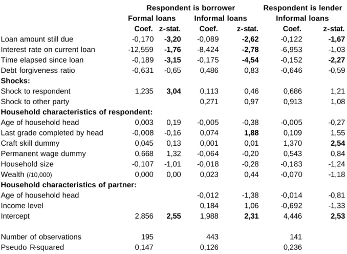
Before concluding, we examine the data for evidence of debt roll-over and over-accumulation of debt. If debt were used to gain economic power over others, the analysis presented in Section 1 would lead us to expect heavily indebted individuals to borrow ever more, hence falling into a debt trap. In contrast, if debt peonage is not part of lenders' strategy, we expect them to refrain from lending to individuals who already owe them a lot of money. By the same token, they should be reluctant to lend to individuals who have taken a long time to pay previous debt and who have already been charged high interest rates in the past.

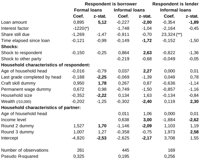
For each loan received, respondents were asked at the end of round 3 whether the lender would be willing to lend them more. For each loan given, on the other hand, respondents were asked whether they would be willing to lend more to the borrower. Overall, some 61% said they would be able to borrow more if they wanted to and 63% said they would agree to lend more if they were asked to. To investigate whether loans tend to snowball, we regress respondents' expectations of future lending on the amount they still owe, the contractual interest rate in their current loan, and the time elapsed since the current loan was granted. Fafchamps and Lund (2002) show that lending often plays an insurance role. To allow for this possibility, we also control for shocks. Loan forgiveness ö is included as regressor as well. If lending is driven by a profit motive, we expect lenders to refrain from lending to individuals who fail to pay their debt in full. In contrast, if lending follows primarily an insurance motive, those who needed debt forgiveness in the past may continue to need assistance in the future.

Results are presented in Table 10. Contrary to the debt peonage model, we find that the amount still due, the interest rate on the current loan, and the time elapsed since the loan was granted all have a negative effect on the expectation of future lending. This is true across all loan categories and whether the respondent is the lender or the borrower. This constitutes fairly convincing evidence that forcing borrowers into high debt is not the strategy pursued by lenders in our sample. It is consistent with the earlier finding that interest charges often are reduced ex post.

We also find some evidence that shocks raise expectations of future lending, confirming the finding of Fafchamps and Lund (2002) that lending plays an insurance role. In the formal lending regression, respondents facing a bad shock expect to borrow more in the future.

Finally, the amount forgiven on the current loan does not have a significant effect on expectations of future lending. The variable even has a positive coefficient in one of the regressions. If anything, this demonstrates that lenders are not 'angry' at delinquent borrowers.

5 . C O N C L U S I O N

In this paper, we have examined the loan repayment practices of rural Filipino households. The literature on rural lending has documented a variety of debt peonage and labor bonding practices. Poor people facing bad shocks are forced to borrow from moneylenders and other strong men in order to survive, only to fall more or less permanently under their control. These practices are typically associated with usurious interest rates, repayment in labor, debt roll-over, and ex post renegotiation of payment terms. We already know that households in our study area borrow to deal with shocks (Fafchamps and Lund 2002). Furthermore, many of the practices associated with debt peonage are present in our data. One objective of this paper was therefore to formally look for evidence of debt peonage or labor bonding in our study area.

In his seminal work on loan repayment in Northern Nigeria, Udry (1994) proposed another vision of rural lending as an insurance vehicle. Building upon the work of Townsend (1993) and others, he argued that contingent loan repayment is an important way by which poor households deal with shocks. According to this view, amounts repaid vary with subsequent shocks to lender and borrower. In contrast, Rosenzweig (1988), Imai (2000) and Fafchamps and Lund (2002) have shown that it is borrowing itself that helps households deal with shocks. This has resulted in some confusion, as it is unclear whether it is debt itself or debt repayment that serves an insurance purpose. A second objective of our research was thus to revisit Udry's claim and examine what dimension of loan repayment is contingent and which is not.

We find little or no support for debt peonage in our study area. The only possible exception concerns the repayment of shop credit in labor, but shop loans seldom carry interest and we find no evidence of debt roll-over and increased indebtedness over time. Contractual interest charges, when present, are seldom fully paid. Lenders refrain from granting new loans to borrowers who have failed to repay old loans, or taken a long time to repay them. Taken together, these findings make it unlikely that surveyed households would fall in a debt trap.14

Our results also put Udry's finding in perspective. By unpacking loan repayment into various components -- timing, amount paid, form of payment, and debt forgiveness -- we were able to clarify the extent to which debt repayment is contingent upon shocks. Contrary to Udry's claim, we do not find that shocks affect the amount repaid or the extent of debt forgiveness. The effect of shocks is primarily through payment delays and repayment in labor: borrowers in difficulty are given more time to pay and allowed to pay part of the loan in labor, usually in the form of an 'advance payment'. The two go together: borrowers work for the borrower when they cannot pay, then pay the remainder in cash at a later date. Debt forgiveness is present in the survey area, but it concerns primarily a reduction in interest charges. This is a far cry from general equilibrium models of contingent credit in which all insurance takes place through contingent repayment (e.g. Townsend 1993, Udry 1992).

In view of the evidence, debt repayment practices in rural Philippines are not that different from what we would observe in corporate America. Borrowers in difficulty are given more time to repay but are requested to demonstrate their good faith in exchange for leniency. The main difference perhaps is that rural Filipino lenders, rather than force a borrower into bankruptcy or debt peonage by accumulating interest charges, choose to reduce interest ex post. This is a priori incompatible with pure profit seeking motive.

Why Filipino lenders display such restraint remains unclear. One possible explanation is that contractual interest is not enforceable due to the informa l nature of the contract. Insisting on full

interest charges may be counterproductive whenever repayment is voluntary and based on an implicit long-term relationship. If this explanation were true, we would expected a difference between formal loans -- for which foreclosure is possible -- and informal loans -- for which it is problematic. Some support for this interpretation can be found in our study area. Another possibility is that lenders and borrowers follow redistributive norms of behavior (Platteau and Hayami 1996). They may be intuitively aware that any debt system in areas with widespread poverty, if unchecked, would naturally lead to debt peonage (Fafchamps 2003). Moral condemnation and other social pressure may prevent lenders from abusing their power, hence forcing them to consent ex post debt reduction. In this sense, the area of the Philippines studied here resembles more Africa than Asia. This issue deserves more research.

References

Banerjee, A. and Munshi, K. (1999), Market Imperfections, Communities, and the Organization of Production: An Empirical Analysis of Tirupur's Garment-Export Network. (mimeograph).

Bardhan, P. (1984), Land, Labor and Rural Poverty, Columbia U.P., New York.

Becker, G.S. and Madrigal, V. (1994), The Formation of Values with Habitual Behavior. (mimeograph).

Ben-Porath, Y. (1980), "The F-connection: Families, Friends, and Firms and the Organization of Exchange.", Population and Development Review, 6(1):1-30.

Bulow, J. and Rogoff, K. (1989a), "A Constant Recontracting Model of Sovereign Debt", J.

Polit.Econ., 97(1):155-178.

Bulow, J. and Rogoff, K. (1989b), "Sovereign Debt: Is to Forgive Forget?", Amer. Econ. Review, 79(1):43-50.

Cochrane, J.H. (1991), "A Simple Test of Consumption Insurance", J. Polit.Econ., 99(5):957-976. de Janvry, A. (1981), The Agrarian Question and Reformism in Latin America, John Hopkins University Press, Baltimore.

Eaton, J. and Gersovitz, M. (1981), "Debt with Potential Repudiation: Theoretical and Empirical Analysis", Review Econ. Studies, XLVIII:289-309.

Eaton, J., Gersovitz, M. and Stiglitz, J. E. (1986), "The Pure Theory of Country Risk". European

Econ. Review, 30:481-513.

Fafchamps, M. (1996), "The Enforcement of Commercial Contracts in Ghana ", World Development 24(3):427-448.

Fafchamps, M. (1999a), "Risk Sharing and Quasi Credit ", Journal of International Trade and

Economic Development, 8(3):257-278.

Fafchamps, M. (1999b), Rural Poverty, Risk, and Development, FAO, Rome. Economic Social Development Paper No. 144.

Fafchamps, M. (2003), Inequality and Risk., Insurance against Poverty, Stefan Dercon (ed.),WIDER, Helsinki. (forthcoming).

Fafchamps, M., Biggs, T., Conning, J. and Srivastava, P. (1994), Enterprise Finance in Kenya. Regional Program on Enterprise Development, Africa Region, The World Bank, Washington, DC. Fafchamps, M. and Lund, S. (2002), "Risk Sharing Networks in Rural Philippines.", Journal of

Development Economics, (forthcoming)

Fafchamps, M., Pender, J. and Robinson, E. (1995), Enterprise Finance in Zimbabwe, Regional Program for Enterprise Development, Africa Division, The World Bank, Washington, DC.

Geertz, C. (1963), Peddlers and Princes: Social Change and Economic Modernization in Two

Indonesian Towns, University of Chicago Press, Chicago.

Genicot, G. (2002), "Bonded Labor and Serfdom: A Paradox of Voluntary Choice.", Journal of

Development Economics, 67(1): 101-27.

Ghate, P. (1992), Informal Finance: Some Findings from Asia, Oxford University Press, for the Asian Development Bank, Manilla.

Grossman, H.I. and Van Huyck, J. B. (1988), "Sovereign Debt as a Contingent Claim: Excusable Default, Repudiation and Reputation. ", Amer. Econ. Review 78(5):1088-1097.

Imai, K. (2000), How Well Do Households Cope with Risk Through Savings and Portfolio Adjustment? Evidence from Rural India. (mimeograph. ).

Kletzer, K. M. (1984), "Asymmetries of Information and LDC Borrowing with Sove reign Risk.",

Econ. J., 94: 287-307.

Kochar, A. (1997), "An Empirical Investigation of Rationing Constraints in Rural Credit Markets in India.", Journal of Development Economics, 53(2):339-371.

Ligon, E., Thomas, J. P. and Worrall, T. (2000), "Mutual Insurance, Individual Savings, and Limited Commitment.", Review of Economic Dynamics, 3( 2):216-246.

Lund, S. (1996), Informal Credit and Risk-Sharing Networks in the Rural Philippines (unpublished Ph.D. thesis).

Mace, B. J. (1991), "Full Insurance in the Presence of Aggregate Uncertainty.", J. Polit. Econ., 99(5):928-956.

Morduch, J. (1995), "Income Smoothing and Consumption Smoothing.” J. Econ. Perspectives 9(3):103-114.

Platteau, J.-P. and Abraham, A. (1987), "An Inquiry into Quasi-Credit Contracts: The Role of Reciprocal Credit and Interlinked Deals in Small-scale Fishing Communities.", J. Dev. Stud., 23(4):461-490.

Platteau, J.-P. and Hayami, Y. (1996), Resource Endowments an Agricultural Development: Africa

vs. Asia, University of Namur and Aoyama Gakuin Universitv, Tokyo, Namur. Paper presented at

the IEA Round Table Conference.

Rosenzweig, M. R. (1988). “Risk, Implicit Contracts and the Family in Rural Areas of Low Income Countries.", Econ. J., 98:1148-1170.

Spagnolo, G. (1995), Social Relations in the Workplace: A 'Linked Games' Approach., Technical

Report, Working Paper No. 76, Working paper Series in Econo mies and Finance, Stockholm

School of Economics, Stockholm.

Srinivasan, T. (1989), On Choice Among Creditors and Bonded Labour Contracts., The Economic

Theory of Agrarian Institutions, Pranab Bardhan (ed.), Clarendon Press, Oxford.

Townsend, R. (1993), Financial Systems in Northern Thai Villages. (mimeograph).

Townsend, R. M. (1994), "Risk and Insurance in Village India.", Econometrica, 62(3):539-591. Udry, C. (1990), "Rural Credit in Northern Nigeria: Credit as Insurance in a Rural Economy.",

World Bank Econ. Rev., 4(3):251-269.

Udry, C. (1992), A Competitive Analysis of Rural Credit: State-Contingent Loans in Northern Nigeria. (mimeo).

Udry, C. (1994). "Risk and Insurance in a Rural Credit Market: An Empirical Investigation in Northern Nigeria.", Rev. Econ. Stud., 61(3):495-526.

Zeller, M., Schrieder, G., von Braun, J. and Heidhues, F. (1993), Credit for the Rural Poor in

Table 1. Income, Gifts, and Loans (over a nine months period)

Mean Coefficient

Sources of Income (pesos) of variation

Non-farm earned income 15 178 1,77

Unearned income (1) 1 818 8,80

Value of annual rice harvest 5 596 2,49

of which, crop sales 226 3,45

Net livestock sales 254 11,22

Gifts and Loans

Gifts received 5 394 1,71

Gifts given 2 569 2,56

Net gifts 2 825 3,72

Net informal borrowing 2 124 2,73

Net gifts and informal borrowing 4 949 2,40

Number of observations 206

(1) Includes rental income, pensions, and sale of some assets. (2) In terms of number of animals, fowl counts for 68%, pigs for 16%, cattle and goats for 1%, and other animals for 14%. The total average value of livestock is 2,605 Pesos and the corresponding coefficient of variation is 1.85.

Table 2. New Loans

(in Pesos per household over the nine months covered by the three survey rounds)

Money flowing

in out

Total, in value 5383 1159

Breakdown by source or destination, in value

With close relatives 6.0% 6.7%

With distant relatives 42.7% 65.8%

With friends and neighbors 18.9% 27.5%

With others 13.0% 0.0%

With formal institutions, etc. 19.4% 0.0%

Table 3. Participation in Informal Credit

Participation during survey Loans

Borrowed at least once over 3 rounds 92%

Lent during at least once over 3 rounds 61%

Borrowed and lent at least once over 3 rnds 54%

Borrowed and lent in same survey round 24%

Did not participate over the three rounds 1%

Repeated Interaction

Repeated loans between rounds 92%

Switched roles in lending (*) 52%

Expect to borrow or lend again from at least

one lender 92%

Number of observations 206

Source: Survey data. (*) Switched between lending and borrowing during the survey.

Table 4. Reason for receiving a loan

(computed on the basis of informal loans over the three survey rounds)

Reason the loan was taken

unweight. _{weighted by} loan value

Consumption 72,8% 53,6%

To pay for household consumption 41,3% 19,3%

To pay for medical expenditures 20,8% 13,8%

To pay for funeral and other ritual expenditures 10,7% 20,6%

Investment 17,2% 31,7%

To pay for school expenditures 10,8% 9,1%

To finance a business or farm investment 4,9% 11,5%

To apply for a job abroad 1,5% 11,1%

Reciprocity 9,6% 14,5%

To repay another loan or gift 3,8% 6,9%

To give another gift or loan 5,9% 7,6%

No reason 0,4% 0,2%

Table 5. Propensity to repay (estimator is duration model)

Respondent is borrower

Respondent is lender

Formal loans Informal loans Informal loans

A. Weibull Hazard z-stat. Hazard z-stat. Hazard z-stat.

Loan amount 0,844 -4,33 0,736 -8,13 0,886 -2,00

Interest factor 0,038 -3,73 0,103 -7,34 0,069 -3,19

Share still due 1,619 1,66 4,140 2,75 3,893 1,85

Shocks:

Shock to respondent 0,814 -1,78 0,863 -1,66 0,852 -1,10

Shock to partner 1,269 2,02 0,774 -1,08

Household characteristics of respondent:

Age of household head 1,019 3,10 1,011 2,06 0,996 -0,50

Last grade completed by head 0,996 -0,18 1,028 1,76 0,984 -0,64

Craft skill dummy 1,290 1,89 1,059 0,55 0,925 -0,40

Permanent wage dummy 1,162 0,81 1,083 0,60 0,933 -0,29

Household size 0,951 -1,18 0,964 -1,26 0,976 -0,45

Wealth (/10,000) 1,021 1,02 1,057 3,05 1,001 0,06

Household characteristics of partner:

Age of household head 1,014 3,57 1,004 0,59

Income level 1,042 0,52 1,365 1,86 p-parameter 0,537 10,81 0,497 13,07 0,287 4,45 B. Cox Loan amount 0,879 -3,36 0,782 -6,49 0,906 -1,64 Interest factor 0,083 -2,77 0,170 -5,31 0,096 -2,62

Share still due 1,305 0,94 3,241 2,36 2,381 1,23

Shocks:

Shock to respondent 0,896 -0,97 0,904 -1,17 0,936 -0,46

Shock to partner 1,315 2,39 0,845 -0,73

Household characteristics of respondent:

Age of household head 1,015 2,43 1,009 1,75 1,002 0,20

Last grade completed by head 0,998 -0,08 1,028 1,75 1,001 0,05

Craft skill dummy 1,242 1,61 1,037 0,34 0,938 -0,34

Permanent wage dummy 1,112 0,56 1,060 0,44 0,911 -0,41

Household size 0,951 -1,21 0,978 -0,77 0,987 -0,25

Wealth (/10,000) 1,014 0,66 1,041 2,19 1,001 0,04

Household characteristics of partner:

Age of household head 1,010 2,71 1,002 0,29

Income level 1,050 0,61 1,262 1,37

Number of observations 639 1217 452

Number of cases of repayment 255 437 165

Time at risk 1631 3227 1248

Dependent variable is time between the time the loan was granted and a repayment was made. Shock to respondent is instrumented (see text).

Table 6. Propensity to repay controlling for individual effects (estimator is duration model with Weibull distribution)

Respondent is borrower Respondent is lender

Formal loans Informal loans Informal loans

A. Shared frailty model Hazard z-stat. Hazard z-stat. Hazard z-stat.

Loan amount 0,791 -4,92 0,721 -7,25 0,804 -2,64

Interest factor 0,011 -4,31 0,067 -7,84 0,037 -3,18

Share still due 2,670 2,90 5,193 3,03 10,375 2,68

Shocks:

Shock to respondent 0,762 -2,05 0,804 -2,17 0,966 -0,20

Shock to partner 1,282 2,04 0,852 -0,62

Household characteristics of respondent:

Age of household head 1,026 2,58 1,015 2,11 0,999 -0,05

Last grade completed by head 1,004 0,14 1,037 1,71 0,982 -0,50

Craft skill dummy 1,135 0,60 1,072 0,49 0,823 -0,65

Permanent wage dummy 1,001 0,00 0,966 -0,18 0,865 -0,41

Household size 0,938 -1,03 0,986 -0,35 1,031 0,34

Wealth (/10,000) 1,033 1,10 1,046 1,89 1,048 1,40

Household characteristics of partner:

Age of household head 1,012 2,79 1,011 1,27

Income level 1,082 0,89 1,391 1,48

p-parameter 0,737 11,86 0,604 14,04 0,604 7,68

theta-parameter (frailty distrib.) -0,779 -2,68 -1,417 -4,76 -0,219 -0,79

B. Fixed effect model

Loan amount 0,797 -3,10 0,669 -5,95 0,728 -2,34

Interest factor 0,000 -5,85 0,026 -8,89 0,009 -3,34

Share still due 5,516 4,21 16,061 4,45 174,222 3,83

Shocks:

Shock to respondent 0,685 -2,10 0,696 -2,74 1,012 0,05

Shock to partner 1,296 1,90 0,769 -0,83

Household characteristics of partner:

Age of household head 1,006 1,12 1,021 1,77

Income level 1,119 0,94 1,137 0,38

p-parameter 1,134 20,79 0,867 21,47 0,978 14,07

Number of observations 639 1217 452

Number of cases of repayment 255 437 165

Table 7. Total amount repaid

(estimator is maximum likelihood selection model)

Respondent is borrower Respondent is lender

Formal loans Informal loans Informal loans

A. Amout repaid Coef. z-stat. Coef. z-stat. Coef. z-stat.

Loan amount 0,852 39,37 0,915 56,99 0,912 31,46

Interest factor 0,511 1,11 0,324 2,62 0,496 1,09

Share still due 0,536 3,52 0,854 4,31 0,738 2,04

Shocks:

Shock to respondent -0,020 -0,32 0,022 0,63 0,122 2,12

Shock to partner 0,097 2,26 0,007 0,06

Household characteristics of respondent:

Age of household head 0,002 0,66 -0,002 -1,04 0,002 0,56

Last grade completed by head -0,002 -0,16 0,000 -0,06 0,005 0,56

Craft skill dummy 0,022 0,28 -0,035 -0,85 -0,053 -0,75

Permanent wage dummy -0,060 -0,59 -0,165 -3,07 -0,181 -2,12

Household size -0,019 -0,83 0,011 0,92 0,000 -0,01

Wealth (/10,000) -0,009 -0,76 0,013 1,92 0,015 2,01

Household characteristics of partner:

Age of household head 0,001 0,91 0,002 0,62

Income level -0,043 -1,43 0,049 0,62

Intercept 0,418 1,77 0,466 2,92 0,163 0,39

B. Selection equation

Loan amount -0,113 -3,65 -0,207 -6,62 -0,083 -1,81

Interest factor -2,646 -4,54 -1,818 -7,23 -1,580 -3,29

Share still due 0,359 1,57 0,899 2,99 0,829 1,92

Time elapsed since loan 0,159 6,55 0,146 8,16 0,031 1,10

Shocks:

Shock to respondent -0,080 -0,63 -0,068 -0,73 -0,141 -0,85

Shock to other party 0,189 1,96 -0,280 -1,59

Household characteristics of respondent:

Age of household head 0,015 2,84 0,007 1,60 0,004 0,61

Last grade completed by head 0,010 0,59 0,024 1,89 0,003 0,17

Craft skill dummy 0,184 1,67 0,004 0,05 0,037 0,26

Permanent wage dummy 0,123 0,79 0,036 0,33 -0,104 -0,59

Household size -0,030 -0,89 -0,021 -0,89 -0,010 -0,24

Wealth (/10,000) 0,006 0,36 0,038 2,30 0,000 0,01

Household characteristics of partner:

Age of household head 0,008 2,72 -0,002 -0,49

Income level 0,074 1,17 0,186 1,35 Round 2 dummy 0,028 0,15 -0,114 -0,81 0,319 1,35 Round 3 dummy 0,159 0,93 0,163 1,27 0,504 2,34 Intercept -0,974 -2,75 -0,552 -1,65 -0,657 -1,24 arctan(rho) 0,298 1,90 0,144 1,06 -0,051 -0,06 ln(sigma) -0,570 -10,92 -0,920 -25,65 -0,949 -15,64 Number of observations 645 1229 463 of which: uncensored 261 445 169

Testing proportionality to amount due

chi-square p-value chi-square p-value chi-square p-value

Coefficient of loan amount=1 46,41 0,0000 28,24 0,0000 9,19 0,0024

Coefficient of interest factor=1 1,14 0,2853 29,71 0,0000 1,22 0,2699

Coefficient of share still due=1 9,30 0,0023 0,54 0,4618 0,52 0,4701

Three coefficients are equal 4,81 0,0905 21,21 0,0000 1,88 0,3905