Algoriths for optimizing shared mobility systems

(1)

HAL Id: pastel-00837006

https://pastel.archives-ouvertes.fr/pastel-00837006

Submitted on 21 Jun 2013

HAL is a multi-disciplinary open access archive for the deposit and dissemination of sci-entific research documents, whether they are pub-lished or not. The documents may come from teaching and research institutions in France or abroad, or from public or private research centers.

L’archive ouverte pluridisciplinaire HAL, est destinée au dépôt et à la diffusion de documents scientifiques de niveau recherche, publiés ou non, émanant des établissements d’enseignement et de recherche français ou étrangers, des laboratoires publics ou privés.

Algoriths for optimizing shared mobility systems

Daniel Chemla

To cite this version:

Daniel Chemla. Algoriths for optimizing shared mobility systems. Operations Research [cs.RO]. Ecole nationale des ponts et chaussées - ENPC PARIS / MARNE LA VALLEE, 2012. English. �pastel-00837006�

(2)

Thèse présentée pour obtenir le grade de

Docteur de l’Université Paris-Est

Spécialité : Mathématiques

par

Daniel Chemla

Ecole Doctorale : MATHÉMATIQUES ETSCIENCES ETTECHNOLOGIES DE

L’INFORMATION ET DE LACOMMUNICATION

ALGORITHMS FOR OPTIMIZING SHARED

MOBILITY SYSTEMS

Thèse soutenue le 19 octobre 2012 devant le jury composé de :

Tal Raviv Rapporteur

Louis-Martin Rousseau Rapporteur

Pierre Carpentier Examinateur

Jean-Philippe Chancelier Examinateur

Dominique Feillet Examinateur

Frédéric Semet Examinateur

Frédéric Meunier Directeur de thèse

(3)

(4)

Dedicated to my grandfathers,

Max Chemla and René Gligseliger

(5)

(6)

La revolucion es como una bicicleta ; si deja de andar, se cae

Che Guevara

Acknowledgements

This PhD was possible thanks to the collaboration of my two advisors Frédéric Meunier at École des Ponts ParisTech and Roberto Wolfler Calvo at Université Paris 13. It received a grant R2DS from the Île-de-France region. I would like to thank my two advisors particularly for their support. I was really lucky to work with them and I really enjoyed it. You were supportive and always available when I needed it.

First of all, I would like to thank Louis-Martin Rousseau and Tal Raviv for their detailled reviews and for coming from abroad to attend my presentation. I would like to thank Pierre Carpentier, Jean-Philippe Chancelier, Dominique Feillet and Frédéric Semet for being part of this jury. During these three years I had the chance to work with other researchers. I would like to thank Aristide Mingozzi who helped me with column generation method and showed me a bit of Emilia Romagna. I would also like to thank Michal Tzur and Tal Raviv who received me in Tel Aviv. In all the visited laboratories I worked together with people I also would like to thank, such as Marianne Trigalo for her comments on my dissertation, Enrico and Guillaume for their help in the ROADEF 2010 Challenge, Antoine for his help and drive in his hippy car, Emanuel and Marco for their helps with SCIP, Zheng for her participation in the Branch-and-Cut algorithm, Roberto for inviting me to the basketball game, Iris, Dana and Reut in TAU for showing me around and Mor for his biking lessons, and Alexandra for the super Canadian TSP and her support and Noam for his computer access. At last I would like to give special thanks to my coworkers, Djamal for having taught me “bâ tâ sâ”, Houssame for his support and the invention of the “glandredie”, Bernat el mejoar and Paolo for their patience during the ROADEF 2012 Challenge, Thomas the best travel agency, Rachana my movie dealer, Pauline and Vincent for their comments. I would like to thank all the members of the CERMICS, LVMT and LIPN departments, especially Nathalie, Catherine and Sylvie for their help. This thesis would not have been possible without Peio who showed me the thesis announcement.

At last I would like to thank Louise, all my friends and my familly for their support. And to my mother who wanted one of her sons to be a physician, “docteur” in French, this misunder-standing has led me here.

(7)

(8)

Abstract

Bikes sharing systems have known a growing success all over the world. Several attempts have been made since the 1960s. The latest developments in ICT have enabled the system to become efficient. People can obtain real-time information about the position of the vehicles. More than 200 cities have already introduced the system and this trend keeps on with the launching of the NYC system in spring 2013. A new avatar of these means of transportation has arrived with the introduction of Autolib in Paris end of 2011.

The objective of this thesis is to propose algorithms that may help to improve this system efficiency. Indeed, operating these systems induces several issues, one of which is the regula-tion problem. Regularegula-tion should ensures users that a right number of vehicles are present at any station anytime in order to fulfill the demand for both vehicles and parking racks. This regulation is often executed thanks to trucks that are travelling the city.

This regulation issue is crucial since empty and full stations increase users’ dissatisfaction. Finding the optimal strategy for regulating a network appears to be a difficult question. This thesis is divided into two parts. The first one deals with the “static” case. In this part, users’ impact on the network is neglected. This is the case at night or when the system is closed. The operator faces a given repartition of the vehicles. He wants the repartition to match a target one that is known a priori. The one-truck and multiple-truck balancing problems are addressed in this thesis. For each one, an algorithm is proposed and tested on several instances. To deal with the “dynamic” case in which users interact with the system, a simulator has been developed. It is used to compare several strategies and to monitor redistribution by using trucks. Strategies not using trucks, but incentive policies are also tested: regularly updated prices are attached to stations to deter users from parking their vehicle at specified stations. At last, the question to find the best initial inventory is also addressed. It corresponds to the case when no truck are used within the day. Two local searches are presented and both aim at minimizing the total time lost by users in the system. The results obtained can be used as inputs for the target repartitions used in the first part.

During my thesis, I participated to two EURO-ROADEF challenges, the 2010 edition pro-posed by EDF and the 2012 one by Google. In both case, my team reached the final phase. In 2010, our method was ranked fourth over all the participants and led to the publication of an article [78]. In 2012, we ranked eighteenth over all the participants. Both works are added in the appendix.

(9)

(10)

Résumé court

Les systèmes de vélos en libre-service ont connu ces dernières années un développement sans précédent. Bien que les premières tentatives de mise en place remontent aux années 60, l’arrivée de technologies permettant un suivi des différents véhicules mis à la disposition du grand public et de l’état des bornes de stationnement en temps réel a rendu ces systèmes plus attractifs. Plus de 200 villes disposent de tels systèmes et cette tendance se poursuit avec l’en-trée en fonctionnement du système de New York prévue pour mars 2013. La fin de l’année 2011 a été marquée par l’arrivée d’un nouvel avatar de ce type de transport avec la mise en place d’Autolib à Paris.

L’objectif de cette thèse est de proposer des algorithmes d’aide à la décision pour l’optimi-sation de réseaux de transport en libre-service. L’exploitation de ces systèmes, qui fleurissent actuellement un peu partout dans le monde, pose en effet de nombreux problèmes, l’un des plus cruciaux étant celui de la régulation. Cette dernière a pour objectif de maintenir dans chaque station un nombre de véhicules ni trop faible, ni trop élevé, afin de satisfaire au mieux la de-mande. Cette régulation se fait souvent par le biais de camions qui effectuent des tournées sur le réseau.

Il apparaît rapidement que la question d’une régulation optimale à l’aide d’une flotte fixée de camions est une question difficile. La thèse est divisée en deux parties. Dans la première partie, le cas “statique” est considéré. Les déplacements de véhicules dus aux usagers sont nég-ligés. Cela traduit la situation la nuit ou lorsque le système est fermé à la location. L’opérateur doit redistribuer les véhicules afin que ceux-ci soient disposés selon une répartition définie. Les problèmes de rééquilibrage avec un ou plusieurs camions sont traités. Pour chacun des deux cas, un algorithme est proposé et utilisé pour résoudre des instances de tailles variées. La seconde partie traite du cas “dynamique” dans lequel les utilisateurs interagissent avec le système. Afin d’étudier ce système complexe, un simulateur a été développé. Il est utilisé pour comparer différentes stratégies de redistribution des véhicules. Certaines utilisent des camions se déplaçant dans la ville pendant la journée. D’autres tentent d’organiser une régulation intrin-sèque du système par le biais d’une politique d’incitation : des prix mis à jour régulièrement encouragent les usagers à rendre leur véhicule dans certaines stations. Enfin, si on choisit de ne pas utiliser de camion durant la journée, la question de la détermination du nombre optimal de véhicules à disposer à chaque station se pose. Deux méthodes de recherche locale visant à minimiser le temps total perdu par les usagers sont présentées. Les résultats obtenus peuvent

(11)

servir pour la définition des répartitions cibles de la première partie.

Durant ma thèse, j’ai pu participer à deux challenges EURO/ROADEF, celui de 2010 pro-posé par EDF et celui de 2012 propro-posé par Google. Dans les deux cas, mon équipe a atteint les phases finales. Lors de l’édition de 2010, notre méthode est arrivée quatrième et a donné lieu à une publication [78]. En 2012, notre méthode est arrivée dix-huitième sur tous les participants. Les travaux menés dans ces cadres sont ajoutés en annexe.

(12)

(13)

(14)

Résumé de la thèse

Les systèmes de vélos en libre-service ont connu ces dernières années un développement sans précédent. Bien que les premières tentatives de mise en place remontent aux années 60, l’arrivée de technologies permettant un suivi des différents véhicules mis à la disposition du grand public et de l’état des bornes de stationnement en temps réel a rendu les systèmes plus attractifs. Plus de 200 villes du monde disposent de tels dispositifs et cette tendance se poursuit avec l’entrée en fonctionnement du système de New York prévue pour mars 2013. La fin de l’année 2011 a été marquée par l’arrivée d’un nouvel avatar de ce type de transport avec la mise en place d’Autolib à Paris.

Si les nouvelles technologies ont permis d’assurer plus de fiabilité dans la localisation des véhicules et de responsabiliser davantage les utilisateurs en traçant l’identité des utilisateurs, elles n’ont toutefois pas résolu le problème des déséquilibres qui peuvent survenir durant la journée. Il n’est en effet pas rare que des stations se retrouvent pleines ou vides pendant des périodes de temps plus ou moins longues. Ces évènements diminuent l’efficacité du système de transport, les utilisateurs se présentant à ces stations ne pouvant pas trouver de véhicules ou de places de parking selon le cas. Le second cas de figure est bien plus préoccupant : un utilisateur qui ne trouve pas de véhicule peut toujours emprunter un autre moyen de transport, alors qu’abandonner son véhicule expose à des pénalités financières. Si ces incidents se re-produisent trop souvent, les utilisateurs risquent tout simplement d’abandonner le système de transport partagé pour lui préférer d’autres moyens de transport plus fiables. Une des difficultés de ces déséquilibres est qu’ils peuvent survenir à différents endroits de la ville selon l’heure de la journée. C’est en effet une conséquence des mouvements pendulaires maison-travail qui ont lieu tous les jours : un quartier d’affaire souffrira d’un trop-plein de véhicules le matin lorsque les employés y arrivent, et d’une pénurie le soir lorsque ces mêmes employés souhaitent rentrer chez eux. La problématique inverse peut se produire dans les quartiers résidentiels.

(21)

d’un réseau de transport partagé. L’objectif de ces travaux est de limiter les évènements “stations pleines” ou “stations vides”. Dans de nombreuses villes déjà, des investissements ont été effectués afin de parer à ces problèmes. Une meilleure gestion des moyens déjà déployés permettrait donc d’améliorer les résultats sans augmenter les coûts. Les problèmes de déséquilibre sont une des principales sources de non-renouvellement des abonnements, comme en témoignent de nombreux articles de presse, tel celui paru dans Le Figaro du 23 mars 2010 [12]. Albert Asseraf, directeur général stratégie, études et marketing de JCDecaux y déclare qu’“il n’est statistiquement pas possible de trouver un vélo ou une place dans 100% des cas”. Si cela reste vrai, on peut toutefois essayer par divers procédés de conserver une bonne couverture de la ville, en évitant que des zones entières souffrent d’excédents ou de carences en véhicules. Dans le cas des systèmes de vélos en libre-service, plusieurs camions parcourent la ville et transportent des vélos. Dans le cas du système Autolib, plus d’une centaine d’employés déplacent les voitures. Ces activités peuvent se faire plus facilement la nuit du fait d’un trafic faible.

Les travaux présentés ici se regroupent en deux parties. La première partie qui regroupe les chapitres 2 et 3 traite de la problématique rencontrée par les opérateurs de ces systèmes la nuit : les véhicules sont répartis sur les stations, mais leur répartition peut être différente de la répartition identifiée comme étant la plus à même de répondre aux besoins de l’heure de pointe du matin. Dans ces deux premiers chapitres, cette répartition cible est une donnée. Le faible nombre d’utilisateur étant présent dans le réseau, leur impact sur le système peut être négligé. Le problème devient alors un problème de redistribution de véhicules des stations ayant un excédent de véhicules vers celles souffrant d’une pénurie de véhicules. La seconde partie regroupe les chapitres 4, 5 et 6. Elle porte sur les problèmes rencontrés en temps réel durant la journée lorsque l’utilisation du système est importante. Le Chapitre 6 traite de l’identification de la répartition permettant de minimiser le temps moyen perdu par les utilisateurs sur toute une journée du fait de ces déséquilibres. Cela peut permettre de proposer une répartition comme cible dans la première partie.

Le Chapitre 2 traite du problème de rééquilibrage d’un réseau avec un unique camion, prob-lème que nous avons appelé le Single-Vehicle One-commodity Capacited Pickup-and-Delivey Problem (SVOCPDP). Pour chaque station, le nombre de véhicules présents est donné, ainsi que le nombre de véhicules souhaités. Cela permet de définir les stations pickup comme celles

(22)

ayant un excédent de véhicule, les stations delivery comme celles ayant une pénurie de véhicule et les stations initially balanced comme celles dont le nombre de véhicules initialement présents est égal au nombre de véhicules souhaités. Un camion se trouve initialement à un dépôt. Il a une capacité et peut donc transporter un nombre borné de véhicules en même temps. L’objectif est de trouver un parcours de coût minimal permettant de déplacer les véhicules des stations pickup vers les stations delivery afin d’atteindre en chaque station le nombre souhaité de véhicule, où le coût d’un circuit est la distance parcourue par le camion.

Dans la littérature, le swapping problem introduit par Anily et Hassin [6] présente des car-actéristiques proches. Différents types d’objets sont disponibles à chaque nœud d’un graphe et d’autres objets sont demandés en ces mêmes nœuds. Deux objets ne peuvent se trouver si-multanément à un même nœud. Un unique camion de capacité unitaire peut déplacer les objets un à un, pouvant les déposer à une station pour revenir les chercher plus tard : c’est la ver-sion préemptive du swapping problem. Celui-ci existe aussi dans une verver-sion non-préemptive, dans laquelle ces dépôts temporaires, appelés drop, sont interdits. Une propriété intéressante est que le camion visite au plus trois fois chaque nœud. Cette propriété est l’idée centrale des méthodes de résolution par algorithme de branch-and-cut proposées par Gendreau et al. pour le résoudre dans ses versions préemptives [20] et non-préemptives [47]. Le SVOCPDP n’a qu’un type d’objets – les véhicules – et des capacités sur chaque station ainsi que sur le camion. La propriété du swapping problem signalée ci-dessus n’est plus valide. Hernandez Pérez et Salazar González [66] ont introduit le One-Commodity Pickup-and-Delivery Travelling Sales-man Problem(1PDTSP). Des objets d’un seul type se trouvent en certains nœuds d’un graphe et doivent être amenés vers d’autres nœuds par un unique camion avec capacité. Celui-ci doit rééquilibrer le graphe en suivant un cycle hamiltonien. Ils proposent des méthodes de résolu-tions heuristiques [68] et une méthode exacte avec un algorithme de branch-and-cut [67].

Le SVOCPDP est proche du 1PDTSP mais il n’impose pas que la solution soit un cycle hamiltonien. Les drops et les splits sont autorisés : la demande à un nœud peut être servie par plusieurs visites. De plus, les stations initially balanced peuvent ne pas être visitées. Un modèle exact est donné pour le SVOCPDP. Celui-ci requiert un grand nombre de variables et donc n’est pas soluble. Une relaxation de ce problème est donnée. Celle-ci peut être résolue grâce à un algorithme de branch-and-cut. Il est prouvé que vérifier si une solution de la relaxation est aussi solution du SVOCPDP est un problème N P-complet. Toutefois, dans la majorité des cas, il y a une solution du SVOCPDP avec un coût proche voire égal au coût de la solution de la relaxation. Plusieurs coupes sont intégrées dans l’algorithme afin de renforcer la solution

(23)

linéaire. Une recherche tabou est utilisée pour trouver des solutions au SVOCPDP. Celle-ci peut se faire en considérant exclusivement la liste des stations à parcourir et non les opérations de chargement ou déchargement à mener à chaque arrêt. Un algorithme de flot maximum permet en effet de reconstruire ces dernières à partir de la suite ordonnée des stations. La recherche tabou est lancée à deux reprises, la première fois à partir d’une solution obtenue par une méthode gloutonne, la seconde fois à partir de la solution obtenue par le branch-and-cut. La méthode est utilisée sur des instances jusqu’à 100 stations et avec diverses valeurs pour les demandes à chaque station. Plusieurs capacités du camion sont testées. Les instances ont été obtenues à partir des instances du 1PDTSP. Des solutions optimales ou proches de la solution optimale sont obtenues en des temps de calcul raisonnables jusqu’à des instances de taille moyenne.

Le Chapitre 3 traite de la résolution du Multiple-Vehicle Balacing Problem (MVBP), ver-sion à plusieurs camions du SVOCPDP. Une flotte homogène de camions est disponible au dépôt. L’objectif est de donner à chaque camion une route à suivre, suite de stations à vis-iter avec des opérations de chargements ou déchargements à effectuer. Le coût d’une route est la distance totale parcourue par le camion. Le but est de rééquilibrer le réseau avec un coût minimal. Afin d’éviter un déséquilibre dans les attributions aux différents camions, les routes ont une taille limitée par un paramètre Rmax. Cela permet de s’assurer de répartir les tâches sur plusieurs camions : en effet, il peut être plus intéressant en terme de coût de n’avoir qu’un unique camion visitant les stations tandis que les autres resteraient au dépôt. Cette borne Rmax marque une différence avec la version monovéhicule. Une seconde différence est l’introduction de la convergence monotone vers l’équilibre : une station pickup ne peut que voir baisser son nombre de véhicules ; inversement, une station delivery ne peut que recevoir des véhicules. Cette contrainte est ajoutée pour éviter des problèmes de coordination entre plusieurs camions où l’un d’eux arriverait à une station pour y prendre des véhicules qui ne sont plus là. Cela interdit les drops, possibles dans la version monovéhicule, mais conserve la propriété de split.

Dans la littérature, le problème le plus proche est le Split Delivery VRP (SDVRP) intro-duit par Dror et Trudeau [35]. L’objectif est de servir plusieurs clients à l’aide d’une flotte homogène de camions présente à un dépôt. Les clients doivent recevoir une certaine quantité d’un produit. Ils peuvent être servis par plusieurs camions : possibilité d’avoir des splits. Le but est de répondre à la demande des clients tout en minimisant la distance totale parcourue par l’ensemble des camions. Dror et Trudeau ont identifié certaines propriétés des solutions

(24)

opti-males. Archetti et al. proposent une recherche tabou [7] et un algorithme exact [9] qui permet de résoudre à l’optimum des instances jusqu’à une quarantaine de clients. La méthode proposée de résolution du MVBP est utilisée sur ces mêmes instances. Dans la littérature, on trouve aussi le Pickup and Delivery Problem with Time Windows (PDPTW) : des objets doivent être collec-tés à des endroits et distribués à d’autres, le tout en respectant des fenêtres de temps. Les points de collecte et de livraison sont couplés, alors que le MVBP est un problème Many-to-Many : tout véhicule peut aller de toute station pickup vers toute station delivery. De très nombreuses méthodes existent pour résoudre le PDPTW. Seule celle de Baldacci et al. [10] est citée ici car elle sert d’inspiration à celle que nous proposons pour la résolution du MVBP.

Avant de présenter un modèle pour résoudre le MVBP, certaines propriétés caractérisant les routes d’une solution optimale sont identifiées. Elles généralisent les propriétés du SDVRP. Ces propriétés appelées règles de dominance vont nous permettent de mieux décrire l’espace des solutions à considérer. Ainsi le nombre d’utilisations des arcs reliant deux stations du même type est borné ; de même, le nombre d’utilisations des arcs reliant des stations de types différents et tels que le camion n’est pas complètement plein ou complètement vide peut être borné. Un modèle set partitioning est ensuite explicité. Néanmoins sa taille étant exponentielle, une méthode de génération de colonnes est mise en œuvre afin de résoudre sa relaxation linéaire. La contrainte d’intégrité des variables de décision est relaxée et seul un sous-ensemble de routes est considéré : c’est le problème maître. Seules les routes susceptibles d’améliorer le coût du problème maître sont ajoutées dans le sous-ensemble des routes considérées. Leur identification se fait par la résolution d’un problème de pricing. La méthode utilisée s’inspire de celle de Baldacci et al. [10]. Des demi-routes aller et retour sont générées par un algorithme d’expansion utilisant des règles de dominances entre demi-routes et une borne de complétion. Cette borne est obtenue par programmation dynamique. Ajoutée au coût d’une demi-route en expansion, on obtient une borne inférieure sur le coût d’une route complète utilisant cette demi-route. Les demi-routes aller et retour compatibles sont ensuite associées afin d’obtenir des routes complètes. Celles dont le coût réduit est négatif sont ajoutées dans le problème maître. Lorsqu’il n’y a plus de route à coût réduit négatif, le problème maître est résolu à l’optimum et la valeur obtenue est une borne inférieure à celle du problème originel. Afin de rehausser cette borne inférieure, différentes inégalités valides sont ajoutées dans la formulation du problème maître. Certaines d’entre elles proviennent de l’utilisation de fonctions dual feasible. Ces fonctions éliminent des solutions du relâché mais pas de solution entière. Une revue sur ces fonctions a été réalisée récemment par Clautiaux

(25)

et al. [26]. Quatre fonctions dual feasible sont utilisées ici : deux d’entre elles proviennent de cet article, les deux autres sont ad hoc. D’autres inégalités introduites sont des inégalités de cliques. Elles reprennent les propriétés de dominance mentionnées précédemment. Les variables duales associées aux premières inégalités peuvent être introduites dans le calcul de la borne de complétion, mais pas les secondes. Une fois toutes les inégalités valides ajoutées, on obtient une nouvelle borne inférieure, plus proche de la solution entière. Afin d’obtenir une borne supérieure, un algorithme mémétique avec découpe optimale est mis en œuvre. Comme dans le cas monovéhicule, il est possible de ne considérer que les suites de stations et de reconstruire les chargements et déchargements à chaque arrêt par un algorithme de flot maximum, qui repose sur un graphe similaire à celui du cas précédent. La méthode de découpe optimale est inspirée de celle de Prins [73]. Les différentes routes sont juxtaposées pour former un grand chromosome. Les opérations de cross-over ont lieu sur ce grand chromosome. L’algorithme de flot maximum de la version monovehicule est alors utilisé sur les nouveaux chromosomes comme s’il s’agissait d’une unique grande tournée. Si une grande tournée n’est pas réalisable, alors quel que soit le découpage, on ne peut pas obtenir de routes permettant le rééquilibrage du réseau, donc le nouveau chromosome est abandonné. Sinon, on cherche à faire un découpage optimal en prenant en compte les distances parcourues grâce à un algorithme de programmation dynamique avec étiquettes. Ce découpage peut ne pas respecter la réalisabilité des routes, mais avec les mouvements de voisinage on la retrouve. Ces mouvements sont des 2-OPT au sein des routes et entre les différentes routes. Une fois une borne supérieure obtenue, on introduit toutes les routes qui sont dans le gap. Cela nous assure d’avoir la solution optimale du problème. Des résultats sont donnés pour des instances allant jusqu’à 40 stations pour un temps d’exécution limité à 6 heures. Les petites instances sont toutes résolues à l’optimum. Sur les instances de taille moyenne, on trouve parfois l’optimum et parfois on ne peut obtenir de garantie d’optimalité de la solution dans le temps imparti. Cela reste vrai sur les grandes instances. Sur les instances du SDVRP résolues par Archetti et al. [9], l’algorithme retrouve 5 des 6 solutions optimales.

La seconde partie traite des problèmes de déséquilibre qui peuvent intervenir durant la journée. L’évolution de la répartition des véhicules dépend fortement de l’utilisation des stations. Par exemple, les impacts sur le réseau de la saturation d’une station sont complexes à évaluer : un utilisateur souhaitant rendre un véhicule à une station pleine va chercher à le restituer dans une station voisine. L’écho d’un problème de saturation ou de pénurie de

(26)

véhicules à une station peut ainsi se propager à tout le réseau. Herbert Simon, Prix Turing 1975 et Prix Nobel en Économie 1978, définit les systèmes complexes [81] comme « un système [. . .] composé d’un grand nombre d’éléments qui interagissent de façon complexe ». Un système de transport partagé entre exactement dans le cadre de ces systèmes.

Afin de pouvoir l’étudier, le Chapitre 4 décrit le simulateur OADLIBSim. Celui-ci permet de simuler facilement l’évolution d’un tel système de transport et de tester différentes stratégies utilisant des camions et/ou des politiques incitatives afin d’améliorer la régulation des véhicules en temps réel. Plusieurs caractéristiques du réseau doivent être fournies au simulateur, comme les paramètres des lois gouvernant les temps nécessaires pour rejoindre une station à partir d’une autre suivant le moyen de déplacement, la matrice Origine-Destination (O-D) régissant les probabilités du choix des destinations pour un utilisateur arrivant à une station ou encore les taux d’arrivée des utilisateurs par station. Différents profils d’utilisateurs peuvent aussi être définis selon leur patience : alors qu’un utilisateur impatient quittera le réseau si la première station qu’il visite n’a pas de véhicule disponible, un utilisateur moins “nerveux” pourra explorer d’autres stations environnantes dans la limite d’un nombre de stations spécifié et d’un temps limite. Le même processus peut avoir lieu lorsqu’il s’agit de rendre un véhicule loué. Enfin, si le choix est fait de mettre en œuvre une politique de prix incitant les utilisateurs à rendre leur véhicule à certaines stations, des paramètres permettent de comparer le coût enduré par un utilisateur se rendant à une station différente de celle initialement choisie. Plusieurs types d’utilisateurs peuvent coexister à l’intérieur du simulateur, les proportions de chacun dans le nombre total d’utilisateurs devant simplement être spécifiées. Le simulateur propose différents indicateurs pour évaluer l’efficacité des différentes méthodes. Les utilisateurs sont recensés selon le service reçu par le système : le nombre d’utilisateurs ayant pu effectivement bénéficier du service dans la limite de leur patience, le nombre d’utilisateurs perdus par manque de véhicules disponibles et ceux perdus par manque de places aux stations visitées. Si des véhicules sont transportés, le ratio du nombre moyen d’utilisateurs satisfaits gagnés sur le nombre de véhicules transportés est aussi calculé. Dans le cas d’une politique incitative, le nombre d’utilisateurs préférant rendre le véhicule à leur station d’origine et effectuer le déplacement à pied est aussi fourni. Ce simulateur programmé en C++ est simple d’utilisation et peut être téléchargé sur le site internet du projet. Des méthodes de régula-tion temps réel peuvent aisément être ajoutées grâce à un template guidant leur implémentarégula-tion.

(27)

Le Chapitre 5 présente différentes méthodes de régulations. Celles-ci ont été implémentées et comparées grâce au simulateur OADLIBSim. Avant de présenter ces méthodes, on prouve que trouver la stratégie permettant de maximiser la probabilité de capter le prochain utilisateur dans le cas ou il y a plusieurs stations vides est un problème N P-complet. Et cela reste vrai si on s’intéresse aux deux prochains utilisateurs. Différentes stratégies heuristiques sont pro-posées. Toutes fonctionnent avec la définition d’un nombre cible de véhicules pour chacune des stations et ont pour objectif de maintenir le nombre de véhicules disponibles aux stations proches de ce nombre cible. Les premières heuristiques proposées utilisent un camion. Celui-ci reçoit comme mission d’aller dans les stations souffrant de déséquilibre afin d’y remédier. Les instructions reçues peuvent être de visiter une ou deux stations selon les cas. Afin d’évaluer les déséquilibres à venir, certaines heuristiques utilisent une prédiction du nombre de véhicules aux stations utilisant les taux d’arrivées des utilisateurs et la matrice O-D. Une autre heuristique recherche la politique optimale à mener afin que l’espérance de retour du système à l’équilibre soit minimale. Le système est décrit comme une chaîne de Markov avec un très grand nombre d’états. L’état tel que les stations sont toutes à l’équilibre peut être décrit comme l’état cible d’un problème de plus court chemin stochastique.

Ce problème est notamment traité dans le livre de Tsitsiklis et Bertsekas [17], où ils ex-posent un algorithme itératif de recherche de politique optimale. Cette méthode est appliquée ici. Elle nécessite toutefois une bonne connaissance de l’évolution de la chaîne de Markov. De façon à réduire son nombre d’états, les stations sont regroupées par cluster. Le comportement des utilisateurs décrit précédemment est rationnel. Dans le cas où un utilisateur arrive à un sta-tion pour louer un véhicule et que celle-ci est vide, mais qu’il y a une stasta-tion pleine à côté, la pénibilité engendrée par ce déplacement peut être négligée. Cela permet de ne plus consid-érer toutes les stations mais seulement un nombre réduit de clusters. Par ailleurs, le nombre exact de véhicules présents au sein d’un cluster peut aussi être négligé. Un cluster sera équili-bré si le nombre de véhicules présents permet d’avoir en moyenne des véhicules et des places disponibles à chaque station. Si le nombre de véhicules est faible, le cluster peut souffrir d’une pénurie de véhicules. Inversement, si ce nombre est grand, une surabondance de véhicules peut entraîner des difficultés pour trouver une place pour les utilisateurs souhaitant rendre leur véhicule. Trois zones sont ainsi définies : déficit de véhicules, équilibre, excès de véhicules. Les décisions quant aux déplacements des camions sont faîtes en regardant l’état de chaque cluster. Le nombre d’états ayant été réduit, le simulateur OADLIBSim est utilisé afin d’approcher la matrice de changement d’état de la chaîne de Markov.

(28)

Une stratégie n’utilisant pas de camion mais un système de prix sur les stations est aussi présentée. Un prix est associé à chaque station . Un utilisateur souhaitant s’y rendre devra s’acquitter de ce prix. Ces prix mis à jour régulièrement servent à dissuader les utilisateurs de se diriger vers les stations déjà fortement occupées pour leur indiquer d’autres stations ayant plus de places disponibles. Le problème de reroutage des utilisateurs est modélisé comme un problème de transport de Monge [61]. Le choix d’utiliser les variables duales de ce problème linéaire pour en faire les prix associés à chaque station permet d’obtenir de bons résultats.

Ces différentes stratégies sont comparées sur un jeu d’instances simulées sur des réseaux réalistes avec un nombre de stations allant de 20 à 250. L’amélioration obtenue par la mise en place de ces stratégies est visible en comparant les performances avec la version sans aucune stratégie temps réel. Les résultats indiquent que dans tel un système évoluant très rapidement, les stratégies à court terme obtiennent de meilleures performances que celles à long terme. Cela peut être déduit en comparant les résultats des différentes méthodes, bien que la méthode de recherche de politique optimale, gourmande en temps de calcul, pâtit aussi de la faiblesse de l’évaluation de la matrice de passage des états de la chaîne de Markov. Par contre, la prise en compte de la prédiction permet d’améliorer les résultats obtenus par rapport aux mêmes méthodes ne se fiant qu’à l’état courant du réseau pour prendre des décisions. Les meilleures performances sont obtenues par la méthode de prix, bien qu’un nombre non négligeable d’utilisateurs préfère ne pas utiliser le système une fois les prix affichés. C’est une des limites de la modélisation à demande inélastique qui suppose que tous les utilisateurs se présentant à une station utilisent effectivement le système.

Le Chapitre 6 aborde la question de la détermination du nombre de véhicules à disposer à chaque station. L’objectif est de trouver la répartition qui minimise le temps moyen perdu par les utilisateurs du fait de problèmes de déséquilibre : un utilisateur se présentant à une station vide pour louer un véhicule devra aller à pied à une autre station afin de trouver un véhicule disponible. Et le même mécanisme se produit pour un utilisateur arrivant à une station pleine souhaitant rendre son véhicule. Le temps perdu peut être mesuré comme la différence entre le temps effectivement mis par un utilisateur pour faire un déplacement et le temps minimal idéal qu’il aurait put mettre si le système était infaillible, le temps de trajet direct de sa station d’origine à sa destination avec le véhicule loué. Dans ce chapitre, on suppose qu’il y aucune politique de régulation temps réel durant toute la période de simulation. Cela peut être le cas dans un système comme Autolib où les activités de repositionnement ont lieu principalement

(29)

la nuit, bien que durant la journée la régulation ait aussi lieu mais en moindre mesure. Les taux d’arrivée à chaque station dépendent ici de la tranche horaire mais pas la matrice O-D. La modification d’une unité du nombre de véhicules initialement disposés à une station peut permettre de parer au premier évènement de pénurie ou d’excès en véhicules qui se produit à la station. Deux différentes méthodes de recherche locale utilisent ce constat. La première conserve le temps perdu à chaque station du fait des problèmes d’excès ou de déficit. La seconde s’intéresse au nombre d’occurrences de ces problèmes. Une fois un grand nombre d’itérations réalisé, le bilan est fait et le nombre de véhicules présent au début de la journée peut être modifié en conséquence. Les deux méthodes sont testées sur des données d’utilisation d’une grande ville américaine, perturbées afin d’obtenir plusieurs instances. Les deux méthodes sont lancées à partir de plusieurs solutions initiales dont l’une est le résultat fourni par l’algorithme de Raviv et Kolka [74] qui cherche à minimiser le nombre d’utilisateurs non satisfaits sur chaque station, sans prendre en compte le report d’utilisateurs d’une station sur ses voisines. Les résultats témoignent d’une robustesse des deux méthodes de recherche qui arrivent à des résultats comparables, indépendamment de leur point de départ.

(30)

(31)

(32)

Chapter 1 Introduction

1.1 Bike sharing system

The urban population increases. In 2009, the level of world urbanization has crossed the 50% line and this movement keeps going on. In the annual report published by the Department of Economic and Social Affairs of the United Nation [65], the level of world urbanization is expected to grow up to 68.7% in 2050. In what is called the “most developed regions”, the rural population has been decreasing for 60 years. This trend is expected to start also in the “less developed regions” after 2025. Meantime, the growth rate of the urban population is positive in both types of regions, though bigger in the later. Governments can try to weaken this imbalance by using decentralization of administrations or by encouraging people and activities to move to rural regions. But effects would only be marginal and the number of mega-cities – metropolitan area with more than 10 billions of inhabitants – is expected to reach 29 in 2050.

As cities will extend themselves, inhabitants will have to cover larger distances to go to the cities centers, their workplaces or leisure facilities. Easy transportation access will become more and more an issue. It is already one in most of the big cities. Zavitsas et al. [88] gather data obtained from 16 cities, most of which are in Europe. They show that economic prosperity is related to efficient urban transportation system and denote problems raised by urban transportation.

One of them is the congestion problem. Congestion has clearly a negative impact as it diminishes the capacity of the existing network. It increases transports emissions as well as the energy-consumption per kilometer and heightens noise pollution. The increasing number of cities with high population density will enhance congestion problems. The authors show that

(33)

the average traffic speed in the Greater London has been decreasing over the last decades, and this is not an isolated case. Congestion is partially explained by people commuting to work or to other activities. This appears clearly as the average traffic speed is even slower during morning and evening peaks. Commuters’ displacements provoke these peaks during which the number of kilometers of traffic jams can be exceptionally huge.

Furthermore, environment preoccupations appeared at the end of last century. Here again, transportation activities play a major role as they are responsible for a quarter of greenhouse gas emissions of the 27 European Union (EU) members states. Moreover, although overall emissions have diminished between 1990 and 2006, emissions due to transportation activities have increased by 27% over this period. In 2009, EU countries agreed on a prospect to reduce their greenhouse gas emission in 2020 by at least 20% below 1990 levels. This commitment cannot be fulfilled without a cut in transportation emissions.

For all these reasons, efficient means of transportation have to be introduced in order to limit today’s congestion and be ready to absorb the arrival of new inhabitants. An increase in the use of personal car would not be an efficient solution as it would worsen the two former problems. EU countries are bound to respect their greenhouse reduction engagements. The environment-friendly Bike Sharing System (BSS) could help. If it cannot replace public transportation, it work as an incentive to stimulate people to change their ground transportation habits. And besides being a green transportation mean, it offers a suitable answer for part of inner-city transportation demand and counters the “last-kilometer problem”. This expression refers to the distance between home and the public transportation system, a distance that can be too far to walk but could be covered by biking. This mean of transportation is not new, however it has a growing success all over the world. Several attempts have been made since the 1960s. Shaheen et al. [80] and DeMaio [31] present a study on this mean of transportation over time and divide the experiments into three generations. The first generation gathers systems, in Europe mainly, where everything is free. People can use bikes and leave them once arrived at their destination in the city centers. No stations are installed. The first realization of this system was done in Amsterdam, Holland, in 1968. Bikes have special distinctive signs such as their color – they usually are painted with one bright color: white in Amsterdam, Holland; yellow in La Rochelle, France; green in Cambridge, UK. But within a few months, most of the bikes are stolen and the others are vandalized. Almost all the experiments have failed. In La Rochelle, France, the system introduced in 1974 met success. The system is still running though slight

(34)

modifications were introduced into the offer in order to trace users [16]. However, this is the first success of bike sharing scheme in Europe. The second generation of systems includes bikes racks. To rent a bike, a small cash deposit has to be done at the station – deposit that is given back to the user when he parks the bike back at a rack. This coin-deposit system was first introduce in Copenhagen, Denmark, in 1995. The deposit was about USD 3. This system is a lot more reliable than its predecessor. However it is much more expensive as it request stations equipments. But users are unidentified. The low price of the deposit did not deter theft and vandalism. As a result, it was canceled in most of the places where it was started, or modified to trace users. The third generation of BSS was enabled thanks to the development of new Information and Communications Technologies (ICT). Bikes are parked at stations racks. To rent a bike, users have to identify themselves by using smart technologies such as mobile phone, membership card, or bank card – the list is not exhaustive. They are charged for the time they use the bike, after a first period during which it is free. Increasing price encourages them to return the bike at a station once their trip is finished. If the bike is not given back, a high punitive cost is charged to the identified user. This generation meets a huge success. The Vélo’v system in Lyon, France, launched in 2005, popularized it. It is the first time a BSS is operated at a large scale: with 1′_{500 bikes at its start, this number has gradually increased}

to reach 3′_{000 bikes. Following Lyon, the French capital city launched its own system,}

Vélib’, in summer 2007. It immediately met a great success with almost 200′_{000 registered}

users and more than 26 millions locations of bikes within the first year. These successes have enhanced this trend and BSSs have appeared in more than 200 cities. This movement keeps going on with the launching of a BSS in New York scheduled for spring 2013. The biggest BSS is in the city of Hangzhou, China, with about 2′_{400 stations and up to 60}′_{000 bikes.}

However, in Paris and some other cities, the system suffers from severe vandalism. More-over, people often find themselves unable to either rent a bike or park it at station because there is no bike parked or no rack available. These issues led to a decrease in the number of users as stated in “Le Figaro” article [12] in 2008 about the Parisian Vélib’ system. In Brus-sels, the Villo! system that opened in 2009 experienced imbalance problems and the press reported them [77]. A website was created by users to measure imbalances in the network (http://www.wheresmyvillo.be).

To reverse this trend, operators engaged themselves to minimize vandalism by reinforcing the equipment and to prevent stations from being full or empty by using real time regulation.

(35)

In the Vélib’ system, the contract that engaged JCDecaux and the city of Paris was modified to include regulation objectives. The demand for transportation can be asymmetrical within the day. This leads to an imbalance of bikes with areas where all stations are full while in others there is a shortage of them. A fleet of trucks is available and turns around the city, moving bikes from a place to another. But how to efficiently plan a regulation system ? How to manage this fleet ? What directions to give to trucks drivers ? Could the system be regulating itself using incentive policies for users ?

1.2 Research motives

Bike sharing problems are relatively new, but there is already an important literature, ad-dressing them from various points of view. Lathia, Ahmad and Capra [56] adopt a statistical approach to discuss the performances of existing systems. Vogel and Mattfeld [84] gather and study data they obtained from the Vienna bike sharing system, and give a model that could be used to further expand the network. Lin and Yang [57] propose a model that gives a strategic planning of a BSS considering a service level requirement. One of the problems BSSs operators face is to balance the network. Depending on days or on locations, some stations or areas of the cities could gather a huge number of bikes, leaving no rack available for users to park. And in other locations, it is the opposite with few bikes available. Moving bikes to balance the network and avoid shortage of bikes or racks is a problem that could fit within the many-to-many pickup and delivery problems class. However, in the daytime, the network is evolving very fast: for example in Paris, there is about 110′_{000 rentals per day in average [2]. The number of bikes}

present at a station may change during the time a truck drives from a station to another. The main reason for long-term subscribers not to renew their subscription is the regulation prob-lem. Several works on that topic have appeared recently, some of which are cited in an article of “Le Temps” printed in 2011 [82]. Raviv et al. [76] propose several models and algorithms to solve a bikes repositioning problem. Their objective is to find the best repositioning that can be achieved by several trucks within time limits, neglecting the impact of users on the system. The satisfaction function introduced by Kolka and Raviv [74] is used to evaluate the quality of a repositioning. Rousseau et al. [27] propose to solve a dynamic public bike sharing balancing problem.

The aim of this thesis is to study efficient algorithms and methods that could be used in operating BSSs and more generally any shared transport system. The focus point is the

(36)

imbal-ances problems as it appears to be a major issue for users. The dissatisfaction of roaming to find a bike or a rack is obvious. The work is separated between the static problem and the dynamic problem. Static problem means that users effect on the system is neglected. It could be the case if the service is closed or overnight when the system is nearly idle as there is almost no users. Note here that several systems around the world are closed during a few hours every days for maintenance and regulation operations. For instance, in Denver, US, the system [3] runs from Mars to December, from 5a.m. to 12a.m. The objective is then to use one or several trucks to balance the system. The problems addressed in the first part belong to the Vehicle Routing Problems class, which is detailed in the next section. On the opposite, dynamic problem refers to the balancing problem when users are in the system and modify the number of vehicles at stations. The question that has to be addressed is how to direct the trucks drivers to have the system providing a good level of service to the users. This is the problem faced at daytime by the operators of these systems. In most of the cities having a BSS, trucks are driving through the city bringing bikes from stations to others. Another problem that popped up is to find the best initial distribution of vehicles to minimize users’ dissatisfaction. Indeed, the trucks impact on the system efficiency can be marginal when a good repartition of the vehicles in the morning could help to reduce dissatisfaction.

1.3 Routing problems and bikes balancing problems

Routing problems gather operational problems faced in the management of distribution tasks. The field of transportation has been one of the major focus of the Operation Research (OR) community. The interest in this topic arose very early. At first, only the savings that can be achieved have motivated to better schedule transportation activities. Growing environment concerns have then enhanced the attractiveness of this field of research. The first and original problem studied is the well-known Travelling Salesman Problem (TSP). Signs of the TSP are found as early as the 1830s in Germany in [19], though this article contains no mathematical treatment. It was named after the problem faced by travelling salesmen who have to visit several cities and so to plan a closed trail – cycle. But to save time or money, they want to find the cycle that would be the less costly for them. The first trace of mathematicians’ interests for the TSP are in the 1930s when it seems to be studied both in Germany and the US. It became in the 1950s and 1960s a very popular topic for researchers.

(37)

while minimizing the total number of kilometers travelled. The distance matrix is given. In 1954, Dantzig et al. [29] presented the optimal cycle linking 49 American cities, one per state + Washington D.C.. They were the first to present a integer linear program and to propose a cutting plane method. This process was later extended with the introduction of branch-and-cut algorithms. In 1962, the society Procter and Gamble ran a contest for finding the optimal cycle reaching 33 American cities. With no surprise, American researchers in OR were listed among the winners. In 1962, Held and Karp [50] presented a dynamic programming approach that successfully solves small size instances. The TSP was proven to be N P-hard in 1972 after Karp proved the N P-completeness of finding an Hamiltonian cycle in a graph, where an Hamiltonian cycle in a graph is a closed trail that visits all vertices once. Since then, the size of instances optimally solved have increased to reach today optimal solution for almost 90′_{000 cities. Huge size instances come from very-large-scale integration problem where a}

huge amount of transistors have to be taken to put them into chips.

Other Vehicle Routing Problems (VRPs) have been defined since the Fifties. More complex than the TSP, they enabled to model and to study different real life transportation problems where other constraints appear. These different features lead to the definition of variants of the TSP, some of them are reported below. The asymmetric TSP is the same problem but where the distance matrix is asymmetric. In the sequential ordering problem, there are precedence constraints on the cities: some cities have to be visited before others.

In the Capacitated Vehicle Routing Problem (CVRP), a fleet of capacitated vehicles is avail-able and to each cities – or customers – a demand is attached. The objective is to find the collection of closed trail such that every customer is visited once and that his demand is satis-fied without exceeding the vehicle capacity. The CVRP first defined in [30] is one of the most studied variant on the TSP. It is a generalization of the TSP. Indeed, the TSP corresponds to an instance with a single vehicle available at the depot which capacity is greater than the sum over the demand of all customers, the depot being the initial city of the tour.

Multiple variants exist on the CVRP or the TSP, adding complications on the tour of the vehicle. In the CVRP case, see [83] for a list of them. Here we give a list of some of them that are relevant with regard to this thesis.

– Associating time windows to customers restrains the visit to occur within time limits. – Enabling the customers to be visited by several vehicles by splitting his demand.

(38)

delivered at vertices. It could be the same or different commodities.

Split means that the demands may be satisfied by several vehicles. The Split Delivery VRP (SDVRP) was first introduced by Dror and Trudeau [35]. As in the CVRP, each customer has a demand that has to be served by capacitated vehicles that are parked at a depot. But vehicles can serve only part of the demand of a customer. Dror and Trudeau proved that the split dimension of the problem could lead to huge savings in term of the objective function [34]. The split component of the problem increases the complexity of the algorithm [8]. However, they found a property that limits the number of solutions to consider. If the costs satisfy the triangle inequality, then there exists an optimal solution to the SDVRP where no two routes have more than one customer with a split delivery in common. Having pickup and delivery requests at vertices leads to different problems depending on specific characteristics. Laporte et al. [15] sort the different Pickup and Delivery Problems (PDPs) that were introduced by different authors. They are sorted with respect to how pickup and delivery vertices are paired or not. Here we will focus on the many-to-many problems. Many-to-many means that pickup and delivery points are not paired. An object picked up at a vertex can be delivered to any other vertex that has a demand for this type of object. Three different problems are in this class.

In the swapping problem, a single vehicle has to move unitary objects from a vertex to another. There are m different types of objects and the vehicle has a unitary capacity: it can only move one object at the time. Each vertex is associated with the type of object currently present at it, if any, and the desired object type, if any. For each type of object, the total demand is assumed to be equal to the total supply. The objective is to find a tour for a unique unit capacity vehicle at the end of which all objects are brought at a vertex where there is a request for an object of their type. This problem was introduced by Anily and Hassin in [6]. They showed that a vertex could be visited at most three times in the optimal solution. The problem has a preemptive version and a non-preemptive version. In the preemptive version, an object can be dropped at a vertex that is not its destination vertex to be collected later on by the vehicle when it comes back.

The second problem in this category is the One-Commodity Pickup-and-Delivery Travel-ling Salesman Problem (1PDTSP). It was first introduced by Hernández-Pérez and Salazar-González in [66]. Vertices are divided into pickup and delivery vertices. There is only one type of commodity. To each vertex is associated a non-zero demand, that is the amount of the

(39)

commodity to either pickup or deliver at the corresponding customer, respectively to its sign. A capacitated vehicle is given at a depot. The objective is to find the minimum Hamiltonian tour that visits once each customer and brings the commodities from pickup vertices to delivery ones. This Hamiltonian tour has to respect the capacity of the vehicle.

The Q-Delivery Travelling Salesman Problem (Q-DTSP) is a special case of the 1PDTSP where all the demands are unit demands. In this case, the demand at pickup or delivery vertices is only one unit of the commodity. It was introduced before the latter in 1999 by Motwani and Chalasani in [63]. Here again, the solution is an Hamiltonian tour. They propose an approximation algorithm to solve it. The same problem was studied at the same time by Anily and Bramel. In [5] they introduce the Capacitated Travelling Salesman Problem with Pickup and Delivery (CTSPPD) as an extension of the swapping problem with one commodity and a capacitated vehicle.

Balancing a shared transport system enters clearly in the many-to-many pickup and delivery problems class. Vehicles have to be moved from stations with an excess of vehicles to stations with a shortage of them. At first glance, the 1PDTSP could model this problem. But there is no reason for not allowing multiple visit at stations. For instance, assume that there is a pickup station where 6 vehicles need to be taken out and that a truck is nearby but has room for only 3 vehicles. Then it could load 3 bikes and come back later to load the others 3. In addition, central stations may be used as buffer where vehicles can be dropped to be recollected later. The 1PDTSP does not allow such operations to occur as its solution is required to be an Hamiltonian cycle. A consequence is also that unfeasible instances of the 1PDTSP could be solved if multiple visits were authorized.

In real time, there are additional constraints on the ways to manage the system. First, the number of bikes changes within the system; second, the computational time of the methods has to be very short to enable to quickly obtain instructions. The VRPs mentioned formerly deal with the static situation. To deal in real time with the dynamic problem faced by a shared transport system operator is another problem. The literature is less developed than in the static case. However, several works have been done on the topic. George and Xia [48] propose a modeling using closed queuing networks. Having an exact model of the system is not an easy task. The latest work using queuing model are done by Fricker and Gast [44]. Pesach et al. [71] propose an dynamic programming algorithm to find the best actions in order to minimize the

(40)

number of unserved users. They use a rolling horizon and launch their program regularly. The work of Contardo et al. [27] formerly mentioned aims also at minimizing the sum of unserved users. They introduce a time-discretized model of the system and use columns generation to obtain in short time instructions to give to the trucks. Here again the method is run regularly.

1.4 Thesis overview

This thesis is organized in two parts and five chapters followed by a chapter containing concluding remarks. Part I consists of chapter 2 and 3 and deals with the static problems. Part II includes chapter 4, 5 and 6 and deals with with the dynamic problems.

In Part I, the static problem is introduced. It is a many-to-many PDPs where the demand at vertices can be split. As stated before, authorizing multiple visits at stations could lead to huge savings in term of the objective function, but it increases the complexity of the problem. Two static problems are formally presented. In this part, the problem is to balance the system during the night with one or several capacitated trucks. These problems suit more to a BSS than a car sharing system. The commodity to move is called bike, and the word vehicle refers to the truck. The Single-Vehicle One-Commodity Pickup and Delivery Problem (SVOCPDP) is the single-vehicle version of the balancing problem. Bikes are initially distributed among the vertices of a graph. To each vertex is associated its initial state, and its target state, where state indicates the number of bikes parked at the vertex. A preliminary discussion with theoretical results such as special polynomial cases or approximation algorithms can be found in the paper by Benchimol et al. [14]. Three types of stations appear; stations which initial state are strictly lower ( respectively greater) than target state are called pickup (respectively delivery) stations; stations which initial state is equal to target state are called initially balanced stations. A capacitated vehicle aims at redistributing the bikes in order to reach a target states distribution. Each vertex can be visited several times and can be moreover used as a buffer in which bikes are stored for a latter visit. The last property allows drops. This many-to-many PDP gathers features from both the 1PDTSP and the swapping problem. The second static problem that is introduced is a multiple-vehicle variant of the latter. It is called Multiple-Vehicle Balancing Problem (MVBP). A fleet of capacitated vehicles is available at a depot. Bikes are distributed over all stations. A target state is given for each station. In the MVBP case, convergence to the target distribution is monotonous: only loading (resp. unloading) operations can occur at

(41)

pickup (resp. delivery) vertices. This last property forbids drops to occur. The objective is to find the set of instructions to give to vehicle drivers that bring the system to its target state while dispatching the tasks to be done over several vehicles and while minimizing the total distance driven.

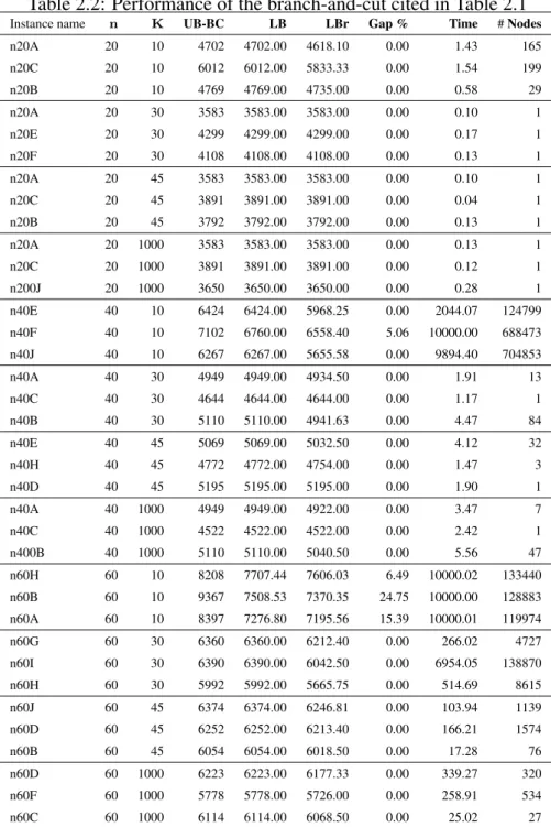
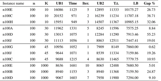
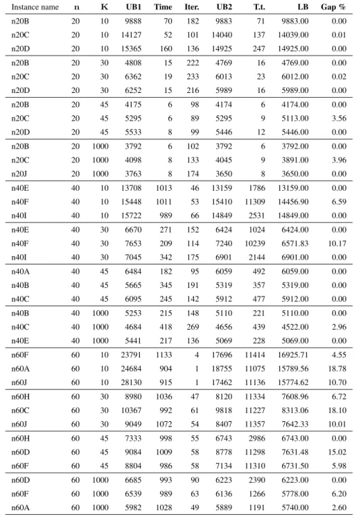
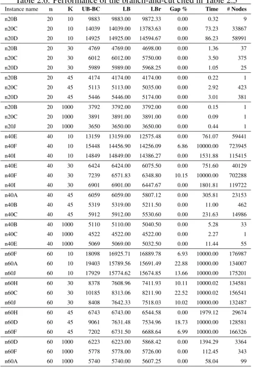
In Chapter 2 the SVOCPDP is studied. Its differences with the swapping problem and the 1PDTSP are explained in detail. A first exact arc-oriented mixed integer programming formulation (MIP) is given. This MIP introduces four sets of variables, some of which are indexed with four indices. The linear relaxation of this model could be very weak and therefore useless, and moreover the model can be intractable. Two consecutive relaxations of the problem are then proposed. They are proven to be equivalent. The meaning of this relaxation is explained, showing that it is a good relaxation, as in most experimental cases, an optimal solution of the relaxation is a solution for the original problem. Several results on the N P-completeness of deciding whether a solution of the relaxation is a solution of the original problem are given. But the last relaxation needs only one set of integer variables, which are the number of times an arc is used. The interest of solving this relaxation appears then clearly. This is solved thanks to a branch-and-cut algorithm. For the branch-and-cut, three separation procedures are used. An upper bound of the optimal solution of the problem is obtained by a tabu search algorithm [49], which is based on some theoretical properties of the solution, once fixed the sequence of the visited stations. It is proven that a solution can be rebuilt knowing only the sequence of visited vertices: bike load can be found using a max-flow algorithm. Computational results are then given for instances with up to 100 vertices, and different capacities for the vehicle. Tests are also done on instances such that the demand at some stations can exceed the vehicle capacity.

Chapter 3 is devoted to the MVBP. Its differences with other pickup and delivery VRPs are emphasized. Several dominances rules and properties of the optimal solutions of the problems are proven. A set partitioning-like model with binary variables is given on the set of all the routes. A route is a tour starting from the depot visiting a subset of vertices with logistic operations to handle at each stop and ending at the depot. The fact that such a model with binary variables exists is not obvious. We can prove that the model is still exact thanks to the dominances aforementioned. However, its linear relaxation is solved with a column-and-cut generation algorithm, since its size being exponential in the size of the instances. The

(42)

relaxation is solved on a subset of variables also called columns. A pricing subproblem is solved to add columns that may improve the cost of the linear relaxation. For that purpose, a two-phase method using dynamic programming is explained. When no more negative reduce cost column can be added, cuts are added to enhance the linear relaxation of the original problem. Once neither cuts nor routes are to be added, a lower bound on the original problem is obtained. A memetic algorithm [62] provides an upper bound on the problem. Then, we add into the subset all columns candidate for being in the optimal solution. They are identified thanks to their reduced cost value. In that case, the original model solved on the subset of routes gives the optimal solution of the original problem. Results are given for instances with up to 40 stations.

Part II deals with the dynamic problem. It refers to the balancing problem in real time. It models the real life problem faced by the operators in the daytime while the system is open. This part is relevant for any shared transport system, so the word vehicle refers this time to the commodity that is shared – bikes in a BSS, cars in a car sharing system – while the word truck is used to represent the regulation activities. In this case, decisions have to be taken regarding balancing vehicles in an uncertain environment. For that purpose, a simulator of shared transport system is described. It models users’ actions on the system. This simulator is used to compare different strategies designed for improving users’ satisfaction. Some of them give instructions to truck driving around the city on where to go and how many vehicles to load or unload at stations. Other strategies use incentives to have the system regulating itself without any truck. Another problem that is studied is the Initial Inventory Problem (IIP). In the IIP, the objective is to find the number of vehicles to deploy in the city and where to deploy them in order to minimize the time users would “lose” using the system, if no regulation activities were done during a time period – a day, a morning.

Chapter 4 describes the simulator OADLIBSim that was developed to model users’ actions in a shared transport system. At first, this mean of transportation is described with its model. The time needed by a vehicle, a truck or a pedestrian to go from vertex i to vertex j are random variables. Users arrive at stations with respect to a Poisson law whose parameters are given. They choose their destination with respect to an O-D matrix. In case users do not find any vehicle at their depart station or any parking place at their destination one, they roam the nearby stations knowing the number of vehicles parked there. Different types of users