ON THE GRENANDER ESTIMATOR AT ZERO
Fadoua Balabdaoui1, Hanna Jankowski2, Marios Pavlides3, Arseni Seregin4 and Jon Wellner4
1Universit´e Paris-Dauphine, 2York University, 3Frederick University Cyprus and 4University of Washington
Abstract: We establish limit theory for the Grenander estimator of a monotone
density near zero. In particular we consider the situation when the true density
f0 is unbounded at zero, with different rates of growth to infinity. In the course of our study we develop new switching relations using tools from convex analysis. The theory is applied to a problem involving mixtures.
Key words and phrases: Convex analysis, inconsistency, limit distribution,
maxi-mum likelihood, mixture distributions, monotone density, nonparametric estima-tion, Poisson process, rate of growth, switching relations.
1. Introduction and Main Results
Let X1, . . . , Xn be a sample from a decreasing density f0 on (0,∞), and let
b
fn denote the Grenander estimator (i.e. the maximum likelihood estimator) of f0. Thus bfn≡ bfnL is the left derivative of the least concave majorant bFn of the
empirical distribution function Fn; see e.g., Grenander (1956a,b), Groeneboom
(1985), and Devroye (1987, Chap. 8).
The Grenander estimator bfnis a uniformly consistent estimator of f0 on sets
bounded away from 0 if f0 is continuous:
sup
x≥c| b
fn(x)− f0(x)| →a.s.0
for each c > 0. It is also known that bfnis consistent with respect to the L1 (kp − qk1 ≡R |p(x) − q(x)|dx) and Hellinger (h2(p, q) ≡ 2−1R hpp(x)−pq(x)
i2 dx)
metrics: that is,
k bfn− f0k1→a.s.0 and h( bfn, f0)→a.s.0;
However, it is also known that bfn(0)≡ bfn(0+) is an inconsistent estimator
of f0(0) ≡ f0(0+) = limx&0f0(x), even when f0(0) < ∞. In fact, Woodroofe
and Sun (1993) showed that b fn(0)→df0(0) sup t>0 N(t) t d = f0(0) 1 U (1.1)
as n→ ∞, where N is a standard Poisson process on [0, ∞) and U ∼ Uniform(0, 1). Woodroofe and Sun (1993) introduced penalized estimators efnof f0 which yield
consistency at 0: efn(0) →p f0(0). Kulikov and Lopuha¨a (2006) study
estima-tion of f0(0) based on the Grenander estimator bfn evaluated at points of the
form t = cn−γ. Among other things, they show that bfn(n−1/3) →p f0(0) if |f0
0(0+)| > 0.
Our view in this paper is that the inconsistency of bfn(0) as an estimator of f0(0) exhibited in (1.1) can be regarded as a simple consequence of the fact that
the class of all monotone decreasing densities on (0,∞) includes many densities
f which are unbounded at 0, so that f (0) = ∞, and the Grenander estimator
b
fn simply has difficulty deciding which is true, even when f0(0) <∞. From this
perspective we seek answers to three questions under some reasonable hypotheses concerning the growth of f0(x) as x& 0.
Q1: How fast does bfn(0) diverge as n→ ∞?
Q2: Do the stochastic processes {bnfbn(ant) : 0 ≤ t ≤ c} converge for some
sequences an, bn, and c > 0?
Q3: What is the behavior of the relative error
sup 0≤x≤cn ¯¯ ¯¯fbn(x) f0(x) − 1 ¯¯ ¯¯ for some constant cn?
It turns out that answers to questions Q1 - Q3 are intimately related to the limiting behavior of the minimal order statistic Xn:1 ≡ min{X1, . . . , Xn}. By
Gnedenko (1943) or de Haan and Ferreira (2006, Thm. 1.1.2)), it is well-known that there exists a sequence {an} such that
a−1n Xn:1→dY, (1.2)
where Y has a nondegenerate limiting distribution G if and only if
for some γ > 0, and hence an→ 0. One possible choice of an is an= F0−1(1/n),
but any sequence {an} satisfying nF0(an) → 1 also works. Since F0 is concave
the convergence in (1.3) is uniform on any interval [0, K]. Concavity of F0 and
existence of f0 also implies convergence of the derivative:
nanf0(anx)→ γxγ−1. (1.4) By Gnedenko (1943), (1.2) is equivalent to lim x→0+ F0(cx) F0(x) = cγ, c > 0. (1.5)
Thus (1.2), (1.3), and (1.5) are equivalent. In this case we have
G(x) = 1− e−xγ, x≥ 0. (1.6) Since F0 is concave, the power γ∈ (0, 1].
As illustrations of our general result, we consider three hypotheses on f0: G0: the density f0 is bounded at zero, f0(0) <∞;
G1: for some β≥ 0 and 0 < C1<∞, (log(1/x))−βf0(x)→ C1, as x& 0;
G2: for some 0≤ α < 1 and 0 < C2 <∞, xαf0(x)→ C2, as x& 0.
Note that in G2 the value α = 1 is not possible for a positive limit C2, since xf (x) → 0 as x → 0 for any monotone density f; see e.g. Devroye (1986,
Thm. 6.2). Below we assume that F0 satisfies the condition (1.5). Our cases G0
and G1 correspond to γ = 1 and G2 to γ = 1− α.
One motivation for considering monotone densities which are unbounded at zero comes from the study of mixture models. An example of this type, as discussed by Donoho and Jin (2004), is as follows. Suppose X1, . . . , Xn are i.i.d.
with distribution function F where,
under H0 : F = Φ, the standard normal d.f.,
under H1 : F = (1− ²)Φ + ²Φ(· − µ), ² ∈ (0, 1), µ > 0.
If we transform to Yi ≡ 1 − Φ(Xi)∼ G, then for 0 ≤ y ≤ 1
under H0 : G(y) = y, the Uniform(0, 1) d.f.,
under H1 : G = G²,µ(y) = (1− ²)y + ²(1 − Φ(Φ−1(1− y) − µ)).
It is easily seen that the density g²,µ of G²,µ, given by g²,µ(y) = (1− ²) + ²
φ(Φ−1(1− y) − µ)
is monotone decreasing on (0, 1) and is unbounded at zero. We show in Section 4 that G²,µ satisfies our key hypothesis (1.5) with γ = 1. Moreover, we show
that the whole class of models of this type with Φ replaced by the generalized Gaussian (or Subbotin) distribution, also satisfy (1.5), and hence the behavior of the Grenander estimator at zero gives information about the behavior of the contaminating component of the mixture model (in the transformed form) at zero.
Another motivation for studying these questions in the monotone density framework is to gain insights for a study of the corresponding questions in the context of nonparametric estimation of a monotone spectral density. In that setting, singularities at the origin correspond to the interesting phenomena of long-range dependence and long-memory processes; see e.g. Cox (1984), Beran (1994), Martin and Walker (1997), Gneiting (2000), and Ma (2002). Although our results here do not apply directly to the problem of nonparametric estimation of a monotone spectral density function, it seems plausible that similar results hold in that setting; note that when f is a spectral density, G1 and G2 corre-spond to long-memory processes (with the usual description being in terms of
β = 1−α ∈ (0, 1) or the Hurst coefficient H = 1−β/2 = 1−(1−α)/2 = (1+α)/2).
See Anevski and Soulier (2011) for recent work on nonparametric estimation of a monotone spectral density.
Let N denote the standard Poisson process on R+. When (1.5), and hence
(1.6) hold, it follows from Miller (1976, Thm. 2.1) together with Jacod and Shiryaev (2003, Thm. 2.15(c)(ii)), that
nFn(ant)⇒ N(tγ) in D[0,∞), (1.7)
which should be compared to (1.3).
Since we are studying the estimator bfn near zero, and because the value
of bfn at zero is defined as the right limit limx&0fbn(x) ≡ bfn(0), it is sensible to
study instead the right-continuous modification of bfn, and this of course coincides
with the right derivative bfnR of the least concave majorant bFn of the empirical
distribution functionFn. Therefore we change notation for the rest of this paper
and write bfn for bfnR throughout. We write bfnLfor the left-continuous Grenander
estimator.
Theorem 1.1. Suppose that (1.5) holds. Let an satisfy nF0(an) ∼ 1, let bhγ denote the right derivative of the least concave majorant of t 7→ N(tγ), t ≥ 0.
Then
(ii) for all c≥ 0, sup 0<x≤can ¯¯ ¯¯ ¯ b fn(x) f0(x) − 1 ¯¯ ¯¯ ¯ →d sup 0<t≤c ¯¯ ¯¯ ¯ t1−γbhγ(t) γ − 1 ¯¯ ¯¯ ¯.
The behavior of bfn near zero under the different hypotheses G0, G1, and
G2 now follows as corollaries to Theorem 1.1. Let Yγ≡ bhγ(0). We then have Yγ= sup
t>0
(N(tγ)/t) = sup
s>0
(N(s)/s1/γ). (1.8)
Here we note that Y1 =d1/U , where U ∼ Uniform(0, 1) has distribution function H1(x) = 1− 1/x for x ≥ 1. The distribution of Yγ for γ ∈ (0, 1] is given in
Proposition 1.5 below. The first part of the following corollary was established by Woodroofe and Sun (1993).
Corollary 1.2. Suppose that G0 holds. Then γ = 1, a−1n = nf0(0+) satisfies nF0(an)→ 1, and it follows that
(i) bfn(0)→df0(0)bh1(0) = f0(0)Y1,
(ii) the processes{t 7→ bfn(tn−1) : n≥ 1} satisfy
b
fn(tn−1)⇒ f0(0)bh1(f0(0)t) in D[0,∞),
(iii) for cn= c/n with c > 0,
sup 0<x≤cn ¯¯ ¯¯ ¯ b fn(x) f0(x) − 1 ¯¯ ¯¯ ¯ →dY1− 1,
which has distribution function H1(x + 1) = 1− 1/(x + 1) for x ≥ 0.
Corollary 1.3. Suppose that G1 holds. Then F0(x)∼ C1x(log(1/x))β so γ = 1, and a−1n = C1n(log n)β satisfies nF0(an)→ 1. It follows that
(i) bfn(0)/(log n)β →dC1Y1,
(ii) the processes{t 7→ (log n)−βfbn(t/(n(log n)β)) : n≥ 1} satisfy
1 (log n)βfbn µ t n(log n)β ¶ ⇒ C1bh1(C1t) in D[0,∞),
(iii) for cn= c/(n(log n)β) with c > 0,
sup 0<x≤cn ¯¯ ¯¯ ¯ b fn(x) f0(x) − 1 ¯¯ ¯¯ ¯ →dY1− 1.
Corollary 1.4. Suppose that G2 holds and set eC2 = (C2/(1− α))1/(1−α). Then F0(x)∼ C2x1−α/(1− α) so γ = 1 − α, a−1n = eC2n1/(1−α) satisfies nF0(an)→ 1, and it follows that
(i) b
fn(0)
nα/(1−α) →dC2e Y1−α, (1.9)
(ii) the processes {t 7→ n−α/(1−α)fbn(tn−1/(1−α)) : n≥ 1} satisfy
b
fn(tn−1/(1−α))
nα/(1−α) ⇒ eC2bh1−α( eC2t) in D[0,∞),
(iii) for cn= c/n1/(1−α) with c > 0,
sup 0<x≤cn ¯¯ ¯¯ ¯ b fn(x) f0(x) − 1 ¯¯ ¯¯ ¯ →d sup 0<t≤c eC2 ¯¯ ¯¯ ¯ tαbh1−α(t) 1− α − 1 ¯¯ ¯¯ ¯.
Taking β = 0 in (i) of Corollary 1.3 yields the limit theorem (1.1) of Woodroofe and Sun (1993) as a corollary; in this case C1 = f0(0). Similarly,
taking α = 0 in (ii) of Corollary 1.4 yields the limit theorem (1.1) of Woodroofe and Sun (1993) as a corollary; in this case C2 = f0(0). Note that Theorem 1.1
yields further corollaries when assumptions G1 and G2 are modified by other slowly varying functions.
Recall the definition (1.8) of Yγ. The following proposition gives the
distri-bution of Yγ for γ∈ (0, 1].
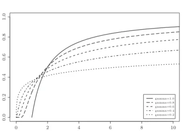
Proposition 1.5. For fixed 0 < γ≤ 1 and x > 0,
Pr µ sup s>0 ½ N(s) s1/γ ¾ ≤ x ¶ = ( 1−1x, if γ = 1, x≥ 1, 1−P∞k=1ak(x, γ) , if γ < 1, x > 0, where the sequence {ak(x, γ)}k≥1 is constructed recursively as follows:
a1(x, γ) = p µµ 1 x ¶γ ; 1 ¶ , and, for j≥ 1, ak(x, γ) = p µµ k x ¶γ ; k ¶ − k−1 X i=1 ½ ai(x, γ)· p µµ k x ¶γ − µ i x ¶γ ; k− i ¶¾ , where p(m; k)≡ e−mmk/k!.
Figure 1. The distribution functions of Yγ, γ∈ {0.2, 0.4, 0.6, 0.8, 1.0}.
Remark 1.6. The random variables Yγ are increasingly heavy-tailed as γ
de-creases; cf. Figure 1. Let T1, T2, . . . be the event times of the Poisson processN,
i.e., N(t) =P∞j=11[Tj≤t]. Then note that
Yγ= supd j≥1 j Tj1/γ ≥ 1 T11/γ ,
where T1∼ Exponential(1). On the other hand Yγ= µ sup t>0 N(t)γ t ¶1/γ ≤ µ sup t>0 N(t) t ¶1/γ d = 1 U1/γ,
where U ∼ Uniform(0, 1). Thus it is easily seen that E(Yγr) < ∞ if and only if
r < γ, and that the distribution function Fγ of Yγ is bounded above and below
by the distribution functions GLγ and GUγ of 1/T11/γ and 1/U1/γ, respectively. The proofs of the above results appear in Appendix A. They rely heavily on a set equality known as the “switching relation”. We study this relation using convex analysis in Section 2. Section 3 gives some numerical results that accompany the results presented here, and Section 4 studies applications to the estimation of mixture models.
2. Switching Relations
In this section we consider several general variants of the so-called switch-ing relation first given in Groeneboom (1985), and used repeatedly by other authors, including Kulikov and Lopuha¨a (2005, 2006), and van der Vaart and Wellner (1996). Other versions of the switching relation were studied by
van der Vaart and van der Laan (2006, Lemma 4.1). In particular, we provide a novel proof of the result using convex analysis. This approach also allows us to re-state the relation without restricting the domain to compact intervals. Through-out this section we make use of definitions from convex analysis (cf., Rockafellar (1970); Rockafellar and Wets (1998); Boyd and Vandenberghe (2004)) that are given in Appendix B.
Suppose that Φ is a function, Φ : D → R, defined on the (possibly infinite) closed interval D ⊂ R. The least concave majorant bΦ of Φ is the pointwise infimum of all closed concave functions g : D → R with g ≥ Φ. Since bΦ is concave, it is continuous on Do, the interior of D. Furthermore, bΦ has left and right derivatives on Do, and is differentiable with the exception of at most countably many points. Let bφL and bφR denote the left and right derivatives,
respectively, of bΦ.
If Φ is upper semicontinuous, then so is Φy(x) = Φ(x)−yx for each y ∈ R. If D is compact, then Φy attains a maximum on D, and the set of points achieving
the maximum is closed. Compactness of D was assumed by van der Vaart and van der Laan (2006, see their Lemma 4.1). One of our goals here is to relax this assumption.
Assuming they are defined, we consider the argmax functions
κL(y)≡ argmaxLΦy ≡ argmaxLx{Φ(x) − yx}
= inf{x ∈ D : Φy(x) = sup z∈D
Φy(z)}, κR(y)≡ argmaxRΦy≡ argmaxRx{Φ(x) − yx}
= sup{x ∈ D : Φy(x) = sup z∈D
Φy(z)}.
Theorem 2.1. Suppose that Φ is a proper upper-semicontinuous real-valued function defined on a closed subset D⊂ R. Then bΦ is proper if and only if Φ ≤ l for some linear function l on D. Furthermore, if conv(hypo(Φ)) is closed, then the functions κL and κR are well defined and for x∈ D and y ∈ R,
S1 bφL(x) < y if and only if κR(y) < x.
S2 bφR(x)≤ y if and only if κL(y)≤ x.
When Φ is the empirical distribution functionFnas in Section 1, then bΦ = bFn
is the least concave majorant ofFn, and bφL= bfnLthe Grenander estimator, while
b
φR = bfn= bfnR is the right continuous version of the estimator. In this situation
the argmax functions κR, κLcorrespond to
bsR
n(y) = sup{x ≥ 0 : Fn(x)− yx = sup z≥0
(Fn(z)− yz)},
bsL
n(y) = inf{x ≥ 0 : Fn(x)− yx = sup z≥0
The switching relation given by Groeneboom (1985) says that, with probability one,
{ bfnL(x)≤ y} = {bsRn(y)≤ x}. (2.1) van der Vaart and Wellner (1996, p.296), say that (2.1) holds for every x and y; see also Kulikov and Lopuha¨a (2005, p.2229), and Kulikov and Lopuha¨a (2006, p.744). The advantage of (2.1) is immediate: the MLE is related to a continuous map of a process whose behavior is well-understood.
The following corollary gives the conclusion of Theorem 2.1 when Φ is the empirical distribution functionFn.
Corollary 2.2. Let bFnbe the least concave majorant of the empirical distribution functionFn, and let bfnL and bfnR denote its left and right derivatives, respectively. Then
{ bfnL(x) < y} = {bsRn(y) < x}, (2.2)
{ bfnR(x)≤ y} = {bsLn(y)≤ x}. (2.3) The following example shows, however, that the set identity (2.1) can fail.
Example 2.3. Suppose that we observe (X1, X2, X3) = (1, 2, 4). Then the MLE is b fnL(x) = 1 3, 0 < x≤ 2, 1 6, 2 < x≤ 4, 0, 4 < x <∞. The process bsRn is given by
bsR n(y) = 4, 0 < y≤ 16, 2, 16 < y ≤ 13, 0, 13 < y <∞.
Note that (2.1) fails if x = 4 and 0 < y < 1/6, since in this case bfnL(x) = bfnL(4) = 1/6 and the event { bfnL(x) ≤ y} fails to hold, while bsRn(y) = 4 and the event
{bsR
n(y)≤ x} holds. However, (2.2) does hold: with x = 4 and 0 < y < 1/6, both
of the events { bfnL(x) < y} and {bsRn(y) < x} fail to hold. Some checking shows that (2.2) and (2.3) hold for all other values of x and y.
Our proof of Theorem 2.1 is based on a proposition that is a consequence of general facts concerning convex functions, as given in Rockafellar (1970) and
Rockafellar and Wets (1998). Let h be a closed proper convex function on R, and let f be its conjugate, f (y) = supx∈R{yx − h(x)}. Let h0−and h0+ be the left and right derivatives of h, and define functions s− and s+ by
s−(y) = inf{x ∈ R : yx − h(x) = f(y)}, (2.4)
s+(y) = sup{x ∈ R : yx − h(x) = f(y)}. (2.5) Proposition 2.4. The following set identities hold:
{(x, y) : h0−(x)≤ y} = {(x, y) : s+(y)≥ x}; (2.6)
{(x, y) : h0+(x) < y} = {(x, y) : s−(y) > x}. (2.7) Proof. All references are to Rockafellar (1970). By Theorem 24.3 the set Γ = {(x, y) ∈ R2 : y ∈ ∂h(x)} is a maximal complete non-decreasing curve. By
Theorem 23.5, the closed proper convex function h and its conjugate f satisfy
h(x) + f (y)≥ xy, and equality holds if and only if y ∈ ∂h(x), or equivalently if x∈ ∂f(y) where ∂h and ∂f denote the subdifferentials of h and f, respectively.
Thus we have Γ ={(x, y) ∈ R2 : x∈ ∂f(x)} and, by the definitions of s− and
s+, Γ ={(x, y) : s−(y) ≤ x ≤ s+(y)}. By Theorem 24.1, the curve Γ is defined
by the left and right derivatives of h:
Γ ={(x, y) : h0−(x)≤ y ≤ h0+(x)}. (2.8) Using the dual representation we obtain
Γ ={(x, y) : f−0 (y)≤ x ≤ f+0 (y)}, (2.9) so s−≡ f−0 and s+≡ f+0 . Moreover, the functions h0−and f−0 are left-continuous,
the functions h0+ and f+0 are right continuous, and all of these functions are nondecreasing.
From (2.8) and (2.9) it follows that {h0−(x) ≤ y} = {f+0 (y) ≥ x}, which implies (2.6). Since the functions h and f are conjugate to each other, the relations between them are symmetric. Thus we have {f−0 (y)≤ x} = {h0+(x)≥
y} or, equivalently, {f−0 (y) > x} = {h0+(x) < y}, which implies (2.7). Before proving Theorem 2.1 we need two lemmas.
Lemma 2.5. Let S = argmaxDΦ and bS = argmaxD bΦ be the maximal super-level sets of Φ and bΦ. Then the set bS is defined if and only if the set S is defined and, in this case, conv(S)⊆ bS.
Proof of Lemma 2.5. Since cl(Φ)≤ bΦ the set S is defined if bS is defined. On
the other hand, if S is defined then Φ is bounded from above on D. Since sup
D
Φ = sup
D
bΦ,
the function bΦ is also bounded from above on D, i.e. the set bS is defined.
By (2.10) we have S ⊆ bS. Since Φ and bΦ are upper semicontinuous the sets
S and bS are closed. Since bS is convex we have conv(S)⊆ bS.
Proof of Lemma 2.6. Indeed, we have conv(hypo(Φ)) ≡ conv(cl(hypo(Φ))),
and conv(hypo(Φ))⊆ hypo(bΦ). Therefore conv(hypo(Φ)) is a hypograph of some closed concave function H such that Φ ≤ H ≤ bΦ. Thus H = bΦ. The set bS is a
face of hypo(bΦ) and the set conv(S) is a face of conv(hypo(Φ)). The statement now follows from Rockafellar (1970, Thm. 18.3).
Proof of Theorem 2.1. To prove the first statement, start with bΦ proper. We have
hypo(Φ)⊆ hypo(cl(Φ)) ≡ cl(hypo(Φ)) ⊆ cl(conv(hypo(Φ))) ≡ hypo(bΦ), (2.10) and therefore hypo(Φ) is bounded by any support plane of hypo(bΦ). This implies that there exists a linear function l such that Φ≤ l.
Now suppose that there is a linear function l such that Φ ≤ l on D. Then cl(Φ) ≤ l and, from (2.10), we have hypo(Φ) ⊆ hypo(l), conv(hypo(Φ)) ⊆ hypo(l), and hypo(bΦ) ≡ cl(conv(hypo(Φ))) ⊆ hypo(l). Thus bΦ < +∞ on D. Since hypo(Φ)⊆ hypo(bΦ) there exists a finite point in hypo(bΦ).
To show that the two switching relations hold, first consider the convex function h = −bΦ. Then bφL(x) = −h0−(x), bφR(x) = −h0+(x), κL(y) = s−(−y),
and κR(y) = s+(−y). By the properness of bΦ proved above and Proposition 2.4,
it suffices to show that
argmaxLx(Φ(x)− yx) = argmaxLx(bΦ(x)− yx), argmaxRx(Φ(x)− yx) = argmaxRx(bΦ(x)− yx).
To accomplish this, it suffices, without loss of generality, to prove the equalities in the last display when y = 0, and this in turn follows if we relate the maximal superlevel sets of Φ and bΦ. This follows from Lemmas 2.5 and 2.6.
Remark 2.7. Note that conv(S) 6= bS in general. To see this, consider the
function
Φ(x) = (
0 x6= 0,
1 x = 0.
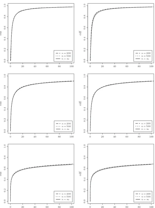
Figure 2. Empirical distributions of the re-scaled MLE at zero when sam-pling from the Beta distribution (left) and the Gamma distribution (right): from top to bottom we have α = 0.2, 0.5, 0.8.
Remark 2.8. Note that if conv(hypo(Φ)) is a polyhedral set, then it is closed
(see e.g., Rockafellar (1970, Corollary 19.1.2)). This is the case in our applica-tions.
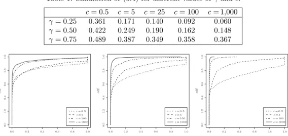
Figure 3. Empirical distributions of the supremum measure: the cutoff values shown are c = 5 (top left), c = 25 (top right), c = 100 (bottom left), c = 1,000 (bottom right).
3. Some Numerical Results
Figure 2 gives plots of the empirical distributions of m = 10,000 Monte Carlo samples from the distributions of bfn(0)/(C2nα/(1− α))1/(1−α)) when n = 200
and n = 500, together with the limiting distribution function obtained in (1.9). The true density f0 on the right side in Figure 2 is
f0(x) = Z ∞ 0 1 y1[0,y](x) yc−1 Γ(c)exp(−y)dy. (3.1) For c∈ (0, 1), this family satisfies (G2) with α = 1 − c and C2 = 1/(αΓ(1− α)). (Note that for c = 1, f0(x)∼ log(1/x) as x & 0.)
The true density f0 on the left side in Figure 2 is
f0(x) = 1
Beta(1− a, 2)x
Table 1. Simulation of (3.4) for different values of γ and c.
c = 0.5 c = 5 c = 25 c = 100 c = 1,000
γ = 0.25 0.361 0.171 0.140 0.092 0.060
γ = 0.50 0.422 0.249 0.190 0.162 0.148
γ = 0.75 0.489 0.387 0.349 0.358 0.367
Figure 4. Empirical distributions of the location where the supremum occurs: from left to right we have γ = 0.25, 0.50, 0.75. Recall that for γ = 1, the (non-unique) location of the supremum is always zero by Corollary 1.2. The data were re-scaled to lie within the interval [0, 1].
For a∈ [0, 1), this family satisfies (G2) with α = a and C2 = 1/Beta(1− α, 2). Figure 3 shows simulations of the limiting distribution
sup 0≤t≤c ¯¯ ¯¯ ¯t1−γ bh(t) γ − 1 ¯¯ ¯¯ ¯ (3.3)
for different values of c and γ. Recall that if γ = 1 the supremum occurs at t = 0 regardless of the value of c, and the limiting distribution (3.3) has cumulative distribution function 1− 1/(x + 1). However, for γ < 1, the distribution of (3.3) depends both on γ and on c, although the dependence on c is not visually prominent in Figure 3. Table 1 shows estimated values of
P à sup 0≤t≤c ¯¯ ¯t1−γbh(t) γ − 1 ¯¯ ¯ = 1 ! (3.4)
for different c and γ < 1, which clearly depends on the cutoff value c (upper bound on the standard deviation in each case is 0.016). Note that (3.3) is equal to one if the location of the supremum occurs at t = 0 (with probability one).
Cumulative distribution functions for the location of the supremum in (3.3) are shown in Figure 4; these depend on both γ and c.
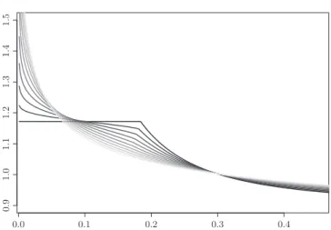
Figure 5. Generalized Gaussian (or Subbotin) mixture densities with ² = .1, µ = 1, r∈ {1.0, 1.2, . . . , 2.0} (black to light grey, respectively) as given by (4.1).
4. Application to Mixtures 4.1. Behavior near zero
Suppose X1, . . . , Xn are i.i.d. with distribution function F , where
under H0 : F = Φr, the generalized normal distribution,
under H1 : F = (1− ²)Φr+ ²Φr(· − µ), ² ∈ (0, 1), µ > 0,
where Φr(x) ≡
Rx
−∞φr(y)dy with φr(y) ≡ exp(−|y|r/r)/Cr for r > 0 gives
the generalized normal (or Subbotin) distribution; here Cr ≡ 2Γ(1/r)r(1/r)−1
is the normalizing constant. If we transform to Yi ≡ 1 − Φr(Xi) ∼ G, then, for
0 ≤ y ≤ 1,
under H0 : G(y) = y, the Uniform(0, 1) d.f.,
under H1: G(y) = G²,µ,r(y) = (1− ²)y + ²(1 − Φr(Φ−1r (1− y) − µ)).
Let g²,µ,r denote the density of G²,µ,r; thus g²,µ,r(y) = 1− ² + ² exp ½ −1 r ¡ |Φ−1 r (1− y) − µ|r− |Φ−1r (1− y)|r ¢¾ . (4.1)
It is easily seen that g²,µ,r is monotone decreasing on (0, 1) and is unbounded at
zero if r > 1. Figure 5 shows plots of these densities for ² = .1, µ = 1, and r ∈
{1.0, 1.1, . . . , 2.0}. Note that g²,µ,1 is bounded at 0, in fact g²,µ,1(y) = 1− ² + ²eµ
Proposition 4.1. The distribution Fµ,r(y)≡ 1 − Φr(Φ−1r (1− y) − µ) is regularly varying at 0 with exponent 1. That is, for any c > 0,
lim
y→0+
Fµ,r(cy) Fµ,r(y)
= c.
Proof. Let κr(y) = Φ−1r (1− y). Our first goal is to show that
lim y→0 κr(y) ˜ κr(y) = 1, (4.2)
where (for y small)
˜ κr(y) = à −r log à Cr y ½ r log µ 1 Cry ¶¾(r−1)/r!!1/r .
To prove (4.2), it is enough to show that lim
y→0κ˜r(y) r−1(κ
r(y)− ˜κr(y)) = 0. (4.3)
This result follows from de Haan and Ferreira (2006, Thm. 1.1.2). Let bn =
˜
κr(1/n), an = 1/bnr−1, and choose F = Φr in the statement of Theorem 1.1.2.
Then, if we can show that
n(1− Φr(anx + bn))→ log G(x) ≡ e−x, x∈ R, (4.4)
it would follow from de Haan and Ferreira (2006, Thm. 1.1.2 and Sec. 1.1.2) that for all x∈ R, lim y→0 U (x/y)− bb1/yc ab1/yc = G −1(e−1/x) = log(1/x),
where U (t) = (1/(1− Φr))−1(t) = Φ−1r (1− 1/t). Choosing x = 1 yields (4.3).
To prove (4.4), we make use of the following, a generalization of Mills’ ratio to the generalized Gaussian family,
1− Φr(z)∼ φr(z)
zr−1 as z→ ∞. (4.5)
This follows from l’Hˆopital’s rule: lim z→∞ R∞ z φr(y)dy z1−rφ r(z) = lim z→∞ −φr(z) (1− r)z−rφr(z) + z1−rφr(z)(−zr−1) = lim z→∞ 1 1− (1 − r)z−r = 1.
Now, n(1− Φr(anx + bn)) ∼ n φr(anx + bn) (anx + bn)r−1 = n Crbrn−1 exp (−(brn/r) (1 + anx/bn)r) (1 + anx/bn)r−1 ∼ n Crbrn−1 exp µ −brn r µ 1 +rx br n ¶¶ = exp µ − µ br n
r + (r− 1) log bn− log n + log Cr
¶¶
exp(−x)
→ exp(−0) · exp(−x)
by using the definition of bn. We have thus shown that (4.2) holds. Then, for y→ 0, by (4.5) and (4.2),
Fµ,r(y) = 1− Φr(κr(y)− µ) ∼ 1 − Φr(˜κr(y)− µ) ∼ φr(˜κr(y)− µ)
(˜κr(y)− µ)r−1 .
Plugging in the definition of φr, we find that
Fµ,r(y)∼ 1/Cr (˜κr(y)− µ)r−1 exp µ −˜κr(y)r r ¯¯ ¯¯1 −κ˜rµ(y)¯¯¯¯r¶ = 1/Cr (˜κr(y)− µ)r−1 exp ½µ
log(Cry) + log(r log(
1 Cry ))¶ ¯¯¯¯1 − µ ˜ κr(y) ¯¯ ¯¯r¶ = 1/Cr (˜κr(y)− µ)r−1 (Cry)|1−µ/˜κr(y)| r · ½ r log 1 Cry ¾[(r−1)/r]|1−µ/˜κr(y)|r .
Note that limy→0˜κr(cy)/˜κr(y) = 1. Therefore,
Fµ,r(cy) Fµ,r(y) ∼ c |1−µ/˜κr(cy)|r · (C ry)|1−µ/˜κr(cy)| r−|1−µ/˜κ r(y)|r · µ ˜ κr(y)− µ ˜ κr(cy)− µ ¶r−1 · n r logC1 rcy o[(r−1)/r]|1−µ/˜κr(cy)|r n r logC1 ry o[(r−1)/r]|1−µ/˜κr(y)|r → c · 1 · 1 · 1 = c.
Thus (1.5) holds with γ = 1.
By the theory of regular variation (see e.g., Bingham, Goldie and Teugels (1989, p. 21)), Fµ,r(y) = y`(y) where ` is slowly varying at 0. It then follows
easily that (1.5) holds for F0 = G²,µ,r with exponent 1. Thus the theory of
Section 1 applies with an of Theorem 1.1 taken to be an= G²,µ,γ(1/n); i.e.
1
n = G²,µ,r(an) = (1− ²)an+ ²Fµ,r(an) ˙= ²Fµ,r(an),
where the last approximation is valid for r > 1, but not for r = 1. When r = 1, the first equality can be solved explicitly, and we find
an=
(
1− Φr(Φ−1r (1− (n²1) + µ), when r > 1, n−1(1− ² + ²eµ)−1, when r = 1.
(4.6)
We conclude that Theorem 1.1 holds for anas in the last display, where bfnis the
Grenander estimator of g²,µ,r based on Y1, . . . , Yn.
Another interesting mixture family is as follows: suppose that Φ1, Φ2 are
two fixed distribution functions, then under H0 : F = Φ1,
under H1 : F = (1− ²)Φ1+ ²Φ2, ²∈ (0, 1).
Using Yi ≡ 1 − Φ1(Xi) ∼ G, then, for 0 ≤ y ≤ 1, we find that under H1 the
distribution of the Yi’s is given by
G(y) = (1− ²)y + ²(1 − Φ2(Φ−11 (1− y))),
g(y) = (1− ²) + ²φ2(Φ −1
1 (1− y)) φ1(Φ−11 (1− y)) .
For Φ2 given in terms of Φ1 by the (Lehmann alternative) distribution function
Φ2(y) = 1− (1 − Φ1(y))γ, this becomes
G(y) = (1− ²)y + ²yγ and g(y) = (1− ²) + ²γyγ−1.
When 0 < γ < 1 this family fits into the framework of our condition G2 with
α = 1− γ and C2= ²γ.
4.2. Estimation of the contaminating density
Suppose that G²,F(y) = (1− ²)y + ²F (y) where F is a concave distribution
on [0, 1] with monotone decreasing density f . Thus the density g²,F of G²,F is
given by g²,F(y) = (1− ²) + ²f(y). Note that g²,F is also monotone decreasing,
and g²,F(y)≥ 1 − ² + ²f(1) = 1 − ² = g²,F(1) if f (1) = 0. For ² > 0 we can write f (y) = g²,F(y)− (1 − ²)
If Y1, . . . , Ynare i.i.d. g²,F, then we can estimate g²,F by the Grenander estimator
bgn, and we can estimate ² by b²n= 1− bgn(1). This results in an estimator of the
contaminating density f , b fn(y) = bg n(y)− (1 − b²n) b²n = bgn(y)− bgn(1) 1− bgn(1) ,
which is quite similar in spirit to a setting studied by Swanepoel (1999). Here, however, we propose using the shape constraint of monotonicity, and hence the Grenander estimator, to estimate both ² and f . We will study this estimator elsewhere.
Appendix A: Proofs for Section 1
For the proof of Theorem 1.1 we need two lemmas. Together, they show that argmaxR and argmaxL are continuous. We assume that (1.5) holds and that nF0(an)∼ 1. Thus both (1.3) and (1.7) also hold.
Lemma A.1. (i) When γ = 1 and x > 1, argmaxL,Rv {nFn(anv)− xv} = Op(1).
(ii) When γ ∈ (0, 1) and x > 0, argmaxL,Rv {nFn(anv)− xv} = Op(1).
Proof. It suffices to show that lim supn→∞P (supv≥K{nFn(anv)−xv} ≥ 0) → 0,
as K→ ∞ under the conditions specified. Let h(x) = x(log x − 1) + 1 and recall the inequality
P (Bin(n, p)/(np)≥ t) ≤ exp(−nph(t))
for t ≥ 1, where Bin(n, p) denotes a Binomial(n, p) random variable; see e.g. Shorack and Wellner (1986, p.415). It follows that
P ( sup v≥K{nFn (anv)− xv} ≥ 0) = P (∪∞j=K{nFn(anv)− xv ≥ 0 for some v ∈ [j, j + 1)}) ≤ ∞ X j=K P (nFn(an(j + 1))− xj ≥ 0) = ∞ X j=K P µ nFn(an(j + 1)) nF0(an(j + 1)) ≥ xj nF0(an(j + 1)) ¶ ≤ ∞ X j=K exp µ −nF0(an(j + 1))h µ xj nF0(an(j + 1)) ¶¶ . (A.1)
Next, since F0 is concave,
nF0(an(j + 1))≤ nF0(an(K + 1)) j + 1 K + 1
for j ≥ K and nF0(an(K + 1))→ (K + 1)γ and n→ ∞. Therefore, for all j ≥ K
and sufficiently large n, we have
xj
nF0(an(j + 1)) ≥ δ(K + 1)
1−γ xj j + 1
for any fixed δ < 1. We need to handle the two cases γ = 1 and γ < 1 sep-arately. Note that if γ < 1, then the above display shows that K, n can be chosen sufficiently large so that (xj)/nF0(an(j + 1)) is uniformly large. On the
other hand if γ = 1 and x > 1, then we can pick δ, K, n large enough so that (xj)/nF0(an(j + 1)) is strictly greater than 1 + ² for some ² > 0, again uniformly
in j.
Suppose first that γ < 1. Then for K, n large, since h(x)∼ x log x as x → ∞, there exists a constant 0 < C < 1 such that for all j≥ K
nF0(an(j + 1))h µ xj nF0(an(j + 1)) ¶ ≥ C(xj) log µ xj j + 1 ¶ ≥ Cx(xj),
for some other constant Cx > 0. This shows that the sum in (A.1) converges to
zero as K→ ∞, as required.
Suppose next that γ = 1. Note that the function h(x) > 0 for x > 1. Therefore, combining our arguments above, we find that for all j≥ K
nF0(an(j + 1))h µ xj nF0(an(j + 1)) ¶ ≥ δ(j + 1)h µ xj nF0(an(j + 1)) ¶ ≥ Cx,δ(j + 1),
again for some Cx,δ > 0. This again implies that the sum in (A.1) converges to
zero as K→ ∞, and completes the proof.
Lemma A.2. Suppose that γ ∈ (0, 1]. Then VxL≡argmaxL v {N(v γ)− xv} =argmaxR v {N(v γ)− xv} ≡ VR x a.s..
Proof. Suppose that VxL < VxR. Then it follows that N((VxL)γ) − xVxL = N((VR
x )γ)− xVxR or, equivalently,
N((VR
x )γ)− N((VxL)γ) = x{VxR− VxL}.
Now (VxR)γ, (VxL)γ ∈ J(N) ≡ {t > 0 : N(t) − N(t−) ≥ 1}, so the left side here takes values in the set{1, 2, . . .} while the right side takes values in x·{r1/γ−s1/γ :
points in J (N) are absolutely continuous with respect to Lebesgue measure, and hence the equality in the last display holds only for sets with probability 0.
Proof of Theorem 1.1. We first prove convergence of the one-dimensional
distributions of nanfbn(ant). Fix K > 0, and let x > 1{γ=1} and t ∈ (0, K]. By
the switching relation (2.3),
P (nanfbn(ant)≤ x) = P (bsLn( x nan )≤ ant) = P (argmaxLs{Fn(s)− xs nan} ≤ an t) = P (argmaxLv{Fn(van)− x( v n)} ≤ t) = P (argmaxLv{nFn(van)− xv} ≤ t) → P (argmaxL v{N(vγ)− xv} ≤ t) = P (bhγ(t)≤ x),
where the convergence follows from (1.7), and the argmax continuous mapping theorem for D[0,∞) applied to the processes {v 7→ nFn(van)− xv : v ≥ 0}; see
e.g. Ferger (2004, Thm. 3 and Corollary 1). Note that Lemma A.1 yields the
Op(1) hypothesis of Ferger’s Corollary 1, while Lemma A.2 shows that equality
holds in the limit.
Convergence of the finite-dimensional distributions of bhn(t) ≡ nanfbn(ant)
follows in the same way by using the process convergence in (1.7) for finitely many values (t1, x1), . . . , (tm, xm), where each tj ∈ R+ and xj > 1{γ=1}.
To verify tightness of bhn in D[0,∞), we use Billingsley (1999, Thm. 16.8).
Thus, it is sufficient to show that for any K > 0, and any ² > 0,
lim M→∞lim supn P Ã sup 0≤t≤K|bh n(t)| ≥ M ! = 0, (A.2) lim δ→0lim supn P ³ wδ,K(bhn)≥ ² ´ = 0. (A.3)
Here wδ,K(h) is the modulus of continuity in the Skorohod topology, wδ,K(h) = inf
{ti}r
max
0<i≤rsup{|h(t) − h(s)| : s, t ∈ [ti−1, ti)∩ [0, K]} ,
where {ti}r is a partition of [0, K] such that 0 = t0 < t1 < . . . < tr = K
and ti− ti−1 > δ. Suppose then that h is a piecewise constant function with
discontinuities occurring at the (ordered) points {τi}i≥0. Then if δ ≤ infi|τi− τi−1| we necessarily have that wδ,K(h) = 0.
First, note that since bhn is non-increasing, kbhnkm0 ≡ sup
0≤t≤m|bhn
(t)| = bhn(0),
and hence (A.2) follows from the finite-dimensional convergence proved above. Next, fix ² > 0. Let 0 = τn,0< τn,1<· · · < τn,Kn < K denote the (ordered)
jump points of bhn, and let 0 = Tn,0< Tn,1<· · · < Tn,Jn < K denote the (again,
ordered) jump points of nFn(ant). Because{τn,1, . . . , τn,Kn} ⊂ {Tn,1, . . . , Tn,Jn},
it follows that inf{τi,n− τi−1,n} ≥ inf{Ti,n− Ti−1,n}, and hence P ³ wδ,K(bhn)≥ ² ´ ≤ P µ inf i=1,...,Jn {Ti,n− Ti−1,n} < δ ¶ .
Now, by (1.7) and continuity of the inverse map (see e.g., Whitt (2002, Thm. 13.6.3)) (Tn,1, . . . , Tn,Jn, 0, 0, . . .)⇒ (T
1/γ 1 , . . . , T
1/γ
J , 0, 0, . . .),
where T1, . . . , TJ denote the successive arrival times on [0, K] of a standard
Pois-son process. Thus lim δ→0P µ inf i=1,...,J{T 1/γ i − T 1/γ i−1} < δ ¶ = 0, and therefore (A.3) holds. This completes the proof of (i).
To prove (ii), fix 0 < c <∞. Write sup 0<x≤can ¯¯ ¯¯ ¯ b fn(x) f0(x) − 1 ¯¯ ¯¯ ¯= sup0<t≤c ¯¯ ¯¯ ¯ nanfbn(tan) nanf0(tan) − 1 ¯¯ ¯¯ ¯. (A.4)
Suppose we could show that the ratio process nanfbn(ant)/nanf0(ant) converges
to the process t1−γbhγ(t)/γ in D[0,∞). Then the conclusion follows by noting
that the functional h7→ sup0<t≤c|h| is continuous in the Skorohod topology as long as c is not a point of discontinuity of h (Jacod and Shiryaev (2003, Prop. VI 2.4)). Since N(tγ) is stochastically continuous (i.e. P (N(tγ)− N(tγ−) > 0) = 0
for each fixed t > 0), t1−γbh
γ(t)/γ is almost surely continuous at c.
It remains to prove convergence of the ratio. Fix K > c, and again we may assume that K is a continuity point. Consider the term in the denominator,
nanf0(ant): it follows from (1.4) that gn(t)≡ (nanf0(ant))−1→ g(t) ≡ γ−1t1−γ,
where g is monotone increasing and uniformly continuous on [0, K]. Thus gn→ g
in C[0, K]. Since the term in the numerator satisfies hn(t) ≡ nanfbn(ant) ⇒
bhγ(t)≡ h(t) in D[0, K], it follows that gnhn⇒ gh in D[0, K], as required. Here,
we have again used the continuity of the supremum. This completes the proof of (ii).
Lemma A.3. Suppose that an = p(1/n) for some function with p(0) = 0 satis-fying limx→0+p0(x)f0(p(x)) = 1. Then nF0(an)→ 1.
Proof. This follows easily from l’Hˆopital’s rule, since lim
n→∞nF0(an) = limx→0+
F0(p(x))
x = limx→0+f0(p(x))p 0(x).
Proof of Corollary 1.2. Under the assumption G0 we see that F0(x) ∼ f0(0+)x as x→ 0, so (1.5) holds with γ = 1. The claim that an = 1/(nf0(0+))
satisfies nF0(an) → 1 follows from Lemma A.3 with p(x) = x/f0(0+). For (i)
note that bh1(0) = bh1(0+) = supt>0(N(t)/t), and the indicated equality in distri-bution follows from Pyke (1959); see Proposition 1.5 and its proof. (ii) follows directly from (i) of Theorem 1.1. To prove (iii), note that from (ii) of Theorem 1.1 that it suffices to show that
sup
0<t≤c
¯¯
¯bh1(t)− 1¯¯¯ =¯¯¯bh1(0+)− 1¯¯¯ = bh1(0+)− 1 = Y1− 1 (A.5)
for each c > 0, where bh1(t) is the right derivative of the LCM of N(t). The
equality in (A.5) holds if bh1(c) > 1, since bh1 is decreasing by definition. By the switching relation (2.3), we have the equivalence{bh1(c) > 1} = {bsL(1) > c}. The equality in (A.5) thus follows ifbsL(1) =∞. That is, if N(t)−t < sup
y≥0{N(y)−y}
for all finite t. Let W = supy≥0{N(y) − y}. Pyke (1959, pp. 570-571) showed that P (W ≤ x) = 0 for x ≥ 0, i.e. P (W = ∞) = 1.
Proof of Corollary 1.3. Under the assumption G1 we see that F0(x) ∼ C1x(log(1/x))β as x → 0, so (1.5) holds with γ = 1. The claim that an =
1/(C1n(log n)β) satisfies nF0(an) → 1 follows from Lemma A.3 with p(x) = x/(C1log(1/x))β. For (i), note that bh1(0) = bh1(0+) = supt>0(N(t)/t), as in the proof of Corollary 1.2. (ii) again follows directly from (i) of Theorem 1.1, and the proof of (iii) is the same as the proof of Corollary 1.2.
Proof of Corollary 1.4. Under the assumption G2 we see that F0(x) ∼ C2x1−α/(1− α) as x → 0, so (1.5) holds with γ = 1 − α. The claim that an={(1 − α)/(nC2)}1/(1−α)satisfies nF0(an)→ 1 follows from Lemma A.3 with p(x) = ((1− α)x/C2)1/(1−α). For (i), note that
bh1−α(0) = bh1−α(0+) = sup t>0 ³N(t1−α) t ´ = sup s>0 ³ N(s) s1/(1−α) ´ ,
much as in the proof of Corollary 1.2. (ii) and (iii) follow directly from (i) and (ii) of Theorem 1.1.
Proof of Proposition 1.5. The part of the proposition with γ = 1 follows from
Pyke (1959, pp. 570-571); this is closely related to a classical result of Daniels (1945) for the empirical distribution function, see e.g. Shorack and Wellner (1986, Thm. 9.1.2).
The proof for the case γ < 1 proceeds along the lines of Mason (1983, pp. 103-105). Fix x > 0 and γ < 1. We aim to establish an expression for the distribution function of Yγ ≡ sups>0(N(s)/s1/γ) at x > 0. First, observe that
P (Yγ≤ x) = P µ sup s>0 ½ N(s) s1/γ ¾ ≤ x 
= P (N(t) ≤ U(t) for all t > 0), (A.6) where the function U (t) = xt1/γ. For j ∈ N, let tj := (j/x)γ and note that t1< t2< . . . and U (tj) = j.
Let B ≡ [N(tk) 6= k ; for all k ≥ 1] and C ≡ [N(s) > U(s) ; for some s > 0].
Then P (B∩ C) = 0 as a consequence of the following argument. Suppose that there exists some t > 0 and k∈ N such that k = N(t) > U(t) and N(ti)6= i, for
all i ≥ 1. It then follows that tk > t, for otherwise k = U (tk) ≤ U(t), as U(·)
is increasing, which is a contradiction. Therefore, tk > t implies that N(tk) >
N(t) = k, as N(·) is non–decreasing and N(tk) = k is disallowed by hypothesis.
Hence N(ti) > i holds for all i ≥ k, for otherwise there would exist some j ≥ k
such thatN(tj) = j, sinceN(·) is a counting process. Therefore, for each i ≥ k we
have that N(s) ≥ i + 1 for all ti ≤ s ≤ ti+1 and, consequently, thatN(s) ≥ U(s)
for all s ≥ tk. This implies that B∩ C ⊆ [lim infs→∞{N(s)/s1/γ} ≥ x] and
therefore P (B∩C) = 0, since the SLLN implies that N(s)/s1/γ → 0 holds almost surely, for fixed γ < 1. Thus P (B∩ C) = 0.
Now P (C) = P (C∩ Bc). Furthermore, since U is a strictly increasing func-tion and since N has jumps at the points {tk} with probability zero, we also
find that P (C∩ Bc) = P (Bc). Finally, write Bc =∪∞k=1Ak for the disjoint sets Ak ≡ [N(tk) = k,N(tj) 6= j for all 1 ≤ j < k], k ≥ 1. Combining the arguments
above, P (Yγ≤ x) = 1 − P (C) = 1 − ∞ X k=1 P (Ak),
where P (A1) = P (N(t1) = 1) = p(t1; 1) and, for k≥ 2, P (Ak) may be written as P (N(tk) = k)− P ({N(tk) = k} ∩ {N(ti)6= i, i < k}c) = P (N(tk) = k)− k−1 X j=1 P (N(tk) = k,N(tj) = j, N(ti)6= i, i < j) = P (N(tk) = k)− k−1 X j=1 P (N(tk)− N(tj) = k− j)P (N(tj) = j,N(ti)6= i, i < j).
The result follows.
Appendix B: Definitions from Convex Analysis
The epigraph (hypograph) of a function f from a subset S ofRdto [−∞, +∞] is the subset epi(f ) (hypo(f )) ofRd+1 defined by
epi(f ) ={(x, t) : x ∈ S, t ∈ R, t ≥ f(x)}, hypo(f ) ={(x, t) : x ∈ S, t ∈ R; t ≤ f(x)}.
The function f is convex if epi(f ) is a convex set. The effective domain of a convex function f on S is
dom(f ) ={x ∈ Rd: (x, t)∈ epi(f) for some t} = {x ∈ Rd: f (x) <∞}. The t-sublevel set of a convex function f is the set Ct = {x ∈ dom(f) : f (x)≤ t}, and the t-superlevel set of a concave function g is the set St={x ∈
dom(g) : g(x)≥ t}. The sets Ct, Stare convex. The convex hull of a set S ⊂ Rd,
denoted by conv(S), is the intersection of all the convex sets containing S. A convex function f is said to be proper if its epigraph is non-empty and contains no vertical lines, i.e., if f (x) < +∞ for at least one x and f(x) > −∞ for every x. Similarly, a concave function g is proper if the convex function −g is proper. The closure of a concave function g, denoted by cl(g), is the
pointwise infimum of all affine functions h ≥ g. If g is proper, then cl(g)(x) = lim supy→xg(y). For every proper convex function f there exists closed proper
convex function cl(f ) such that epi(cl(f ))≡ cl(epi(f)). The conjugate function
g∗ of a concave function g is defined by g∗(y) = inf{hx, yi − g(x) : x ∈ Rd}, and the conjugate function f∗ of a convex function f is defined by f∗(y) = sup{hx, yi − f(x) : x ∈ Rd}. If g is concave, then f = −g is convex and f has conjugate f∗(y) =−g∗(−y).
A complete non-decreasing curve is a subset ofR2 of the form Γ ={(x, y) : x ∈ R, y ∈ R, ϕ−(x)≤ y ≤ ϕ+(x)}
for some non-decreasing function ϕ fromR to [−∞, +∞] that is not everywhere infinite. Here ϕ+ and ϕ− denote the right and left continuous versions of ϕ,
respectively. A vector y∈ Rdis said to be a subgradient of a convex function f at a point x if f (z)≥ f(x) + hy, z − zi for all z ∈ Rd. The set of all subgradients
of f at x is called the subdifferential of f at x, and is denoted by ∂f (x). A face of a convex set C is a convex subset B of C such that every closed line segment in C with a relative interior point in B has both endpoints in B. If B is the set of points where a linear function h achieves its maximum over C, then B is a face of C. If the maximum is achieved on the relative interior of a line segment L⊂ C, then h must be constant on L and L ⊂ B. A face B of this type is called an exposed face.
References
Anevski, D. and Soulier, P. (2011). Monotone spectral density estimation. Ann. Statist. 39, to appear. arXiv:0901.3471v1.
Beran, J. (1994). Statistics for Long-Memory Processes, Vol. 61 of Monographs on Statistics and
Applied Probability. Chapman and Hall, New York.
Billingsley, P. (1999). Convergence of Probability Measures. 2nd edition. Wiley, New York. Bingham, N. H., Goldie, C. M. and Teugels, J. L. (1989). Regular Variation. Vol. 27 of
Ency-clopedia of Mathematics and its Applications. Cambridge University Press, Cambridge.
Boyd, S. and Vandenberghe, L. (2004). Convex Optimization. Cambridge University Press, Cambridge.
Cox, D. R. (1984). Long-range dependence: A review. In Statistics: An Appraisal (H. A. David and H. T. David, eds.). Iowa State University.
Daniels, H. E. (1945). The statistical theory of the strength of bundles of threads. I. Proc. Roy.
Soc. London. A 183, 405–435.
de Haan, L. and Ferreira, A. (2006). Extreme Value Theory. Springer, New York.
Devroye, L. (1986). Nonuniform Random Variate Generation. Springer-Verlag, New York. Devroye, L. (1987). A Course in Density Estimation. Vol. 14 of Progress in Probability and
Statistics. Birkh¨auser Boston Inc., Boston, MA.
Donoho, D. and Jin, J. (2004). Higher criticism for detecting sparse heterogeneous mixtures.
Ann. Statist. 32, 962–994.
Ferger, D. (2004). A continuous mapping theorem for the argmax-functional in the non-unique case. Statist. Neerlandica 58, 83–96.
Gnedenko, B. (1943). Sur la distribution limite du terme maximum d’une s´erie al´eatoire. Ann.
of Math. 44, 423–453.
Gneiting, T. (2000). Power-law correlations, related models for long-range dependence and their simulation. J. Appl. Probab. 37, 1104–1109.
Grenander, U. (1956a). On the theory of mortality measurement. I. Skand. Aktuarietidskr. 39, 70–96.
Grenander, U. (1956b). On the theory of mortality measurement. II. Skand. Aktuarietidskr. 39, 125–153.
Groeneboom, P. (1985). Estimating a monotone density. In Proceedings of the Berkeley
confer-ence in honor of Jerzy Neyman and Jack Kiefer, Vol. II. Wadsworth, Belmont, CA.
Jacod, J. and Shiryaev, A. N. (2003). Limit Theorems for Stochastic Processes. Vol. 288 of
Grundlehren der Mathematischen Wissenschaften [Fundamental Principles of Mathemati-cal Sciences], 2nd ed. Springer-Verlag, Berlin.
Kulikov, V. N. and Lopuha¨a, H. P. (2005). Asymptotic normality of the Lk-error of the
Grenan-der estimator. Ann. Statist. 33, 2228–2255.
Kulikov, V. N. and Lopuha¨a, H. P. (2006). The behavior of the NPMLE of a decreasing density near the boundaries of the support. Ann. Statist. 34, 742–768.
Ma, C. (2002). Correlation models with long-range dependence. J. Appl. Probab. 39, 370–382. Martin, R. J. and Walker, A. M. (1997). A power-law model and other models for long-range
dependence. J. Appl. Probab. 34, 657–670.
Mason, D. M. (1983). The asymptotic distribution of weighted empirical distribution functions.
Miller, D. R. (1976). Order statistics, Poisson processes and repairable systems. J. Appl.
Prob-ability 13, 519–529.
Pyke, R. (1959). The supremum and infimum of the Poisson process. Ann. Math. Statist. 30, 568–576.
Rockafellar, R. T. (1970). Convex Analysis. Princeton University Press, Princeton, N.J. Rockafellar, R. T. and Wets, R. J.-B. (1998). Variational Analysis. Vol. 317 of Grundlehren
der Mathematischen Wissenschaften [Fundamental Principles of Mathematical Sciences].
Springer-Verlag, Berlin.
Shorack, G. R. and Wellner, J. A. (1986). Empirical Processes with Applications to Statistics. John Wiley & Sons Inc., New York.
Swanepoel, J. W. H. (1999). The limiting behavior of a modified maximal symmetric 2s-spacing with applications. Ann. Statist. 27, 24–35.
van de Geer, S. (1993). Hellinger-consistency of certain nonparametric maximum likelihood estimators. Ann. Statist. 21, 14–44.
van der Vaart, A. and van der Laan, M. J. (2006). Estimating a survival distribution with current status data and high-dimensional covariates. Int. J. Biostat. 2, 42.
van der Vaart, A. W. and Wellner, J. A. (1996). Weak Convergence and Empirical Processes. Springer-Verlag, New York.
Whitt, W. (2002). Stochastic Process Limits. Springer-Verlag, New York.
Woodroofe, M. and Sun, J. (1993). A penalized maximum likelihood estimate of f (0+) when f is nonincreasing. Statist. Sinica 3, 501–515.
Centre de Recherche en Math´ematiques de la D´ecision, Universit´e Paris-Dauphine, Paris, 75775, France.
E-mail: [email protected]
Department of Mathematics and Statistics, York University, Toronto, Ontario M3J 1P3, Canada. E-mail: [email protected]
School of Engineering and Applied Sciences, Frederick University Cyprus, Nicosia, 1036, Cyprus. E-mail: [email protected]
Department of Statistics, University of Washington, Seattle, WA 98195, USA E-mail: [email protected]
Department of Statistics, University of Washington, Seattle, WA 98195, USA. E-mail: [email protected]