This is a publisher-deposited version published in: http://oatao.univ-toulouse.fr/
Eprints ID: 3233
To cite this document: SANCHES, Leonardo. MICHON, Guilhem. BERLIOZ,
Alain. ALAZARD, Daniel. Instability zones identification in multiblade rotor
dynamics. In: 11th Pan-American Congress of Applied Mechanics, 04-08 Jan 2010,
Foz do Iguaçu, Brazil.
Any correspondence concerning this service should be sent to the repository
administrator:
[email protected]
INSTABILITY ZONES IDENTIFICATION IN MULTIBLADE ROTOR
DYNAMICS
Leonardo Sanches, [email protected]
Guilhem Michon, [email protected]
Université de Toulouse, ISAE – DMSM – CP: 31055, Toulouse, France
Alain Berlioz, [email protected]
Université de Toulouse, INSA-UPS, LGMT, EA814 - 118 route de Narbonne, CP: 31 077, Toulouse, France
Daniel Alazard, [email protected]
Université de Toulouse, ISAE – DMIA – CP: 31055, Toulouse, France
Abstract. Helicopter ground resonance is an unstable dynamic phenomenon which can lead to the total destruction of
the aircraft during take-off or landing phases. Studies have been developed by researchers which considered a simplified mathematical model. With the goal of further comprehend the phenomenon, predictions of unstable motions are done and compared. First, Floquet’s theory is applied to solve the linear equations of motion including parametric and periodic terms. Then, the multiple scales method is applied on the nonlinear model. The analyses highlight that, by keeping the nonlinear terms in the equations, other instability zones are identified.
Keywords: Ground Resonance, Nonlinear Dynamics, Floquet Method, Multiple Scales Method.
1. INTRODUCTION
The ground resonance phenomenon in helicopters consists of a self-excited oscillation caused by the interaction of the rotor blades’ lagging motion with other helicopter modes of motion. Several accidents have been recorded and show that, under some conditions, it can be very violent and can lead to the total destruction of the aircraft.
Coleman and Feingold (1958) performed some of the earliest research on the phenomenon, and laid the foundation for all of the work that was to follow. Between those, Donham et al. (1969), and Lytwyn et al. (1969) studied this phenomenon taking into account also the air resonance effect. Major contributions in understanding the ground resonance phenomenon in hingeless and bearingless rotors were done by Army researchers, as for example, Dawson (1983) and Hodges (1979). Recently, Kunz (2002) analysed the influence of nonlinear springs and dampers (elastomeric elements) on predicting the rotor’s instability zone. Byers and Gandhi (2006) explored the passive control of the problem.
However, in order to establish the criteria to avoid the unstable oscillations, the equations of motion were linearized and then simplified by eliminating the periodic and parametric termes. This last process, applicable only for isotropic systems, is identified as the Coleman Transformation and more generally called the multi blade coordinate transformation.
A recent study given by Skjoldan et al. (2009) kept the periodic and parametric terms in the equations of motion of a wind turbine. The instability zone predicted by using the Floquet’s theory over a certain range of rotation speeds is similar to that predicted by Coleman and Feingold, for a isotropic rotor.
With the objective of further understanding the ground resonance phenomenon, an analysis of the nonlinear equations of motion is envisioned. This paper sets up the nonlinear equations of motion by considering all terms. Multiple scales method is used to treat the equations of motion.
2. MECHANICAL MODEL
Similar to that proposed by Coleman and Feingold, the present mechanical model is developed to characterize the
dynamical behavior of a helicopter with a hinged rotor. In other words, it consists of figuring out the relation between the longitudinal – x(t) - and lateral displacement – y(t) - of the fuselage, and the kth blade lag angle - ϕk(t) – in terms of the rotor speed Ωand time t. Figure 1illustrates a general schema of the system.
The fuselage is considered to be a rigid body with its center of gravity at point O. At the initial time, the origin of an inertial coordinate system (X0,Y0,Z0) is coincident at this point. The body is connected to springs which represent the
flexibility of the landing skid.
The rotor head system consists of an assembly of one rigid rotor hub with Nb blades. Each blade is represented by a concentrated mass located at a distance b from the lag articulation (point B) and, on each articulation, a torsional spring is present. The origin of a mobile coordinate system (x, y, z), parallel to the inertial one, is located at the geometric center of the rotor hub (point A). Both, body and rotor head, are joined by a rigid shaft and the aerodynamical forces on the blades are neglected.
Yo Kb_X O Xo Zo Kb_Y φk Ω Fuselage Rotor Blade Linear Springs Torsional Spring x y B A Yo Kb_X O Xo Zo Kb_Y φk Ω Fuselage Rotor Blade Linear Springs Torsional Spring x y B A Figure 1. General schema of the mechanical model
2.1 Equation of motion
The equations of motion are obtained by applying Lagrange’s equation on the kinetic and potential energy expressions of the system (body and rotor head). To reach this goal, some conditions have been considered, which are:
• The fuselage has mass mf and the spring constants connected to it are Kf-X and Kf-Y through x and y
directions, respectively;
• The rotor is composed of Nb = 4 blades and each blade k has an azimuth angle of θk =2π
(
k−1)
Nbwith the x - axis;
• Each blade has the same mass mb and moment of inertia around the z - axis is to Izb ; • The angular spring constant for each k blade is Kb-k;
• The k blade position projected in the inertial coordinate system is:
xb_k =acos(Ωt+θk)+bcos(Ω θt+ k+ϕk(t))+x(t) (1)
yb_k =asin(Ωt+θk)+bsin(Ω θt+ k +ϕk(t))+y(t) (2)
where a is the hinge offset.
Considering the general Laplace variable q as
{
q1..6(t)}
{
1(t) 2(t) 3(t) 4(t)}
{
u1..6(t)}
T T
x(t) y(t) ϕ ϕ ϕ ϕ
= = (3)
where u is a vector made up of the degree of freedom variables of the system.
Equations (4 - 6), are nonlinear equations in the function of u. Equations (4) and (5) correspond to the motion equation in the x and y directions, respectively. Equation (6) represents the dynamical equations of blades 1 to 4, changing n from 3 to 6 in that order.
(
) (
)
(
) (
)
(
) (
)
(
) (
)
(
)
2 2 1 2 2 2 2 2 d (t) (t) dt d dcos sin (t) (t) sin cos (t) (t)
dt dt
d d
2 cos cos (t) (t) 2 sin sin (t) (t)
dt dt sin si 1 1 m n 2 n n m n 2 n n m n 2 n n m n 2 n n m n 2 u u r b Ωt u u r b Ωt u u Ωr b Ωt u u Ωr b Ωt u u r b Ωt ω θ θ θ θ θ − − − − − + − + − + − + + + + + +
(
)
(
) (
)
(
) (
)
(
) (
)
2 2 2 2 0 d d n (t) (t) cos cos (t) (t) dt dtcos cos (t) sin sin (t)
6 n 3 n n m n 2 n n m n 2 n m n 2 n u u r b Ωt u u Ω r b Ωt u Ω r b Ωt u θ θ θ = − − − = − + − + + +
∑
(4)(
) (
)
(
) (
)
(
) (
)
(
) (
)
(
)
2 2 2 2 2 2 2 2 d (t) (t) dt d dcos cos (t) (t) sin sin (t) (t)
dt dt
d d
2 cos sin (t) (t) 2 sin cos (t) (t)
dt dt sin cos 2 2 m n 2 n n m n 2 n n n 2 n n m n 2 n n m n 2 u u r b Ωt u u r b Ωt u u Ω αb Ωt u u Ωr b Ωt u u r b Ωt ω θ θ θ θ θ − − − − − + + + − + − + − + + − +
(
)
(
) (
)
(
) (
)
(
) (
)
3 2 2 2 2 0 d d (t) (t) cos sin (t) (t) dt dtcos sin (t) sin cos (t)
6 n n n m n 2 n n m n 2 n m n 2 n u u r b Ωt u u Ω r b Ωt u Ω r b Ωt u θ θ θ = − − − = − + − + − +
∑
(5)(
)
(
) (
)
(
) (
)
(
) (
)
(
) (
)
2 2 2 1 2 2 2 2 1 2 2 2 2 2 2 d d(t) (t) sin (t) sin cos (t) (t)
dt dt
d d
cos sin (t) (t) cos (t) (t)
dt dt d sin sin (t) (t) 0 dt 2 n n n b n b n 2 n b n 2 n b n 2 n b n 2 n u u r a Ω u r Ωt u u r Ωt u u r cos Ω t u u r Ωt u u ; ω θ θ θ θ − − − − + + − + − + + + − + = 3 6 n= ... (6) where 12 _ 22 _ 3..62 _1..4 2 1 , , f X , f Y , b b m b f b f b f b b b K K K m r r b m Nb m ω m Nb m ω m Nb m ω b m Iz = = = = = + + + +
The terms ω1 and ω2 are the resonance frequency of the fuselage in the x and y directions, respectively. Moreover, ω3..6are the resonance frequencies of blades 1 to 4. The terms rm and rb are smaller than one.
3. FLOQUET’S METHOD
In this section a simplified mathematical model is expanded. A Taylor’s series of first order is developed for the terms sin(un) and cos(un) in the equations (4-6) and, furthermore, the nonlinear terms are neglected. Consequently, a
new dynamical system is reached, and is represented as below. ext
M u G uɺɺ+ ɺ+K u=F (7)
where M is the inertia matrix, G is the damping matrix, K is the stiffness matrix, and Fext is the external vector force.
Due to the fact that parametric terms exist, M becomes a symmetric and non-diagonal matrix, G and Kare non-symmetric and non-diagonal matrices. Also, because of the rotor head’s symmetry, Fext is equal to zero.
Then, Floquet’s theory is used to solve differential equations with periodic coefficients. Considering S(t), the state-space matrix with period T of Eq. (7), and its state-state-space representation as
[
]
0 0 0 ( ) ( ) ( ) , ( ) , ( ) ( ) ( ) v S v v v v u u T t t t t t t t t t = > = = ɺ ɺ (8)By Floquet’s Theory, a transition matrixΦ, which relates v( )t and
0 ( ) vt , is defined as
( ) ( )
(
0)
0 0 , , Q Φ t t =P t t et t− (9)The monodromy matrix R and the constant matrix Q are defined, then:
(
0 ,0)
R=Φ t +T t and Q 1log
( )
R TThe dynamical system Eq. (7) is stable if the eigenvalues (µ) of Q are negative or, similarly, if the norm of the eigenvalues of R is less than one.
4. MULTIPLE SCALES METHOD
The perturbation method used to obtain the solution for these nonlinear equations is the multiple scales method (Nayfeh, 2004). It consists of assuming that in any function dependent of time, the independent variable t is a function of multiple scales of the time at the first order. Then, the perturbation substitutions created by introducing a bookkeeping parameterε are:
; 6 .. 1 ) , ( ) , ( ) ( 0 1 0 1 1 0 + = = T T T T n t n n n u u u ε (11) , , m b R r =ε α r =ε β Ω Ω= +ε σ (12)
where, ΩR is the nominal rotor speed, σ is the detuning frequency parameter of the rotation speed and the terms T0 and
T1 correspondent to t and εt, respectively.
The terms sin(un) and cos(un) are expanded by a Taylor’s series of first order in u and, after that, the perturbation
substitutions are done on the equations of motion. Consequently, several sets of equations are obtained by grouping them by power of ε.
4.1. Order ε0 equations
The set of order ε0 equations of the system is collected. They represent the steady-state response of the uncoupled rotor and fuselage system.
(
)
(
)
0 0
2 2
0 0 1 0 1
D un T T, +ωnun T T, =0, n=1..6 (13)
where D0 is the derivative with respect to T0.
The solutions of these equations are trivial and are in the form of
( )
0[ ]
0 1 1 . , 1..6 2 n I T n n u A T e ω c c n = + = , since the
steady-state responses are zero. The term An(T1) is complex and defined asA Tn( )1 =C T en( )1 −I B Tn( )1 , where Cn and Bn
are the amplitude and phase angle of each response, respectively.
4.2. Order ε1 equations
The following, Eq. (14-16), is the set equations of order ε1.
(
)
(
)
( )
(
)
(
)
(
)
(
)
(
)
(
)
(
(
)
)
(
)
(
)
(
)
(
)
(
)
(
)
(
)
( )
1 1 0 1 0 1 0 0 0 0 1 0 1 0 0 1 0 0 2 2 0 1 0 1 1 1 0 1 3 2 2 0 0 1 0 0 1 0 1 2 2 2 2 0 0 1 2 2 3 0 0 1 0 D , , 1 D , D , 2 , 1 1 D , 2 2 1 D , D 2 R R R R R I Ω T T I Ω T T n n n R n n I T T I T T n n n R I T T n n n R n u T T u T T I b u T T e I b u T T e u T T I b u T T e I b e I b u T T e I b u T σ σ Ω σ Ω σ Ω σ ω α α Ω α α Ω α α Ω + + − − + + − − + − − + = + + + − + +(
)
(
)
( )
(
(
)
)
(
)
[ ]
0 1 0 1 0 6 3 0 1 2 3 0 0 1 , . 1 D , 2 R R I T T n I T T n n T e c c I b u T T e Ω σ Ω σ α + = + − + + ∑
(14)(
)
(
)
(
)
(
)
(
)
( )
(
)
(
)
( )
(
(
)
)
(
)
( )
(
)
(
)
( )
(
)
(
)
(
)
1 1 0 1 0 1 0 0 0 0 1 0 1 0 0 1 0 0 2 2 0 2 0 1 2 2 0 1 2 2 3 0 0 1 0 0 1 0 1 2 3 3 2 0 0 1 3 2 2 0 0 1 0 D , , 1 D , D , 2 , 1 1 D , 2 2 1 D , D 2 R R R R R I T T I T T n n n R n n I T T I T T n n n R I T T n n n R n u T T u T T I b u T T e I b u T T e u T T I b u T T e I b e I b u T T e I b u Ω σ Ω σ Ω σ Ω σ Ω σ ω α α Ω α α Ω α α Ω + + − − + + − − + − − + = − + + + − − +(
)
(
)
(
)
(
(
)
)
(
)
[ ]
0 1 0 1 0 6 3 0 1 2 2 0 0 1 , . 1 D , 2 R R I T T n I T T n n T T e c c I b u T T e Ω σ Ω σ α + = + − + − ∑
(15)(
)
(
)
( )
(
)
(
)
(
)
(
)
(
)
(
)
(
)
(
)
(
)
( )
(
)
(
)
[ ]
1 1 0 1 0 1 0 0 0 0 1 0 1 0 0 2 2 0 0 1 0 1 3 2 2 2 0 1 0 1 0 2 0 1 0 1 2 2 3 2 0 1 0 1 0 2 0 1 D , , 1 1 D , D , , 2 2 1 1 D , D , . 3..6 2 2 R R R R n n n I T T I T T n n n I T T I T T n n u T T u T T I u T T e I u T T e u T T I u T T e I u T T e c c n Ω σ Ω σ Ω σ Ω σ ω β β β β + + − − + + − − + = − + − − + = (16)where [c.c] corresponds to the complex conjugate of the previous terms.
As observed, the right-hand side of the above equations is all dependent on the steady-state responses
0
n
u .
4.3. Secular terms – possible instable regions
The developing of Eq. (14-16), after Eq. (13) have been substituted into them, lead to combinations of ωn and ΩR multiplied by T0 as exponent to each equation of motion. Therefore, depending on the applied specific rotor speedΩR,
secular terms may exist. This fact implies that the response(s)
1
n
u grows without limit as t increases and, consequently, it does not provide a small correction to
0
n
u .
Based on that, a set of possible rotor speed values ofΩRfor each equation is listed and it indicates instability zones of the system. These zones are well defined through the analysis of the amplitude responses calculated around a critical value forΩR by shifting the detuning frequency parameter.
Body’s Equation – Eq. (14): 0 ω1 ω1±ωn ω1±2ωn ω1±3ωn n=3..6 (17)
Body’s Equation – Eq. (15): 0 ω2 ω2±ωn ω2±2ωn ω2±3ωn n=3..6 (18)
Blade’s Equations – Eq. (16): ω1,2 ω1,2−ωn ω1,2−2ωn n=3..6 (19)
5. RESULTS
The goal of this section is to predict and collect the speed rotor valueΩRfor which the system becomes instable from
both mathematical models developed previously. Later, the results are compared. The numerical values used for the system’s inputs are defined in Tab. 1.
Table 1. Numerical values of the fuselage and rotor head inputs
Fuselage Rotor
mf = 2902.9 [kg] mb = 31.9 [kg] a = 0.2 [m] b = 2.5 [m]
Kf-X = Kf-Y = 1.077e3 [kN/m] Kb-1..4 = 40.716 [kNm/rad] Izb = 259 [kg m2]
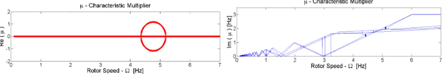
Applying the numerical values, the resonance frequency, in Hz, of the fuselage ω1 and ω2 are equal to 3.00 and, for the bladesω3,ω4,ω5andω6 are equal to 1.50. By varying the rotor speed from 0 to 7 Hz, Fig. 2 illustrates the instability zone for 4.358<Ω<5.187, in Hz, by using Floquet’s Method. It is defined when the real part of the characteristic multipliers are positive and nonzero.
Figure 2. Campbell Diagram by Floquet Method.
However, by using Multiple Scales Method, the rotor speed values in Hz, at which unstable oscillations for the fuselage and the blades may occurs, are ordered as follow:
R
Ω =
[
1.5 3.0 4.5 6.0 7.5]
(20)6. CONCLUSION
As for the comprehension and analysis, this paper envisioned to verify the influence of the nonlinear terms in the equations of motion on the prediction of the rotor speed which the ground resonance phenomenon may occur. Two different models were developed and compared: one keeps the linear, parametric and periodic terms and another considers all terms, including the nonlinear ones.
The numerical results obtained in the first model, by applying the Floquet’s Theory, show a well defined instability zone for the rotor speed between 4.358 and 5.187 Hz. Time response analysis for Ω=4.77 Hz evidences the divergent behaviour of the fuselage displacement.
However, the analysis of the secular terms in the nonlinear model, by using multiple scales method, verifies many others possibilities of instability zones. They are defined as a combination of the resonance frequency of the fuselage and the blades’, by considering the linear system of motion as uncoupled. It evidences the importance of considering the nonlinear terms into the model in order to predict the instability zones.
The perspectives for this work consist in studying the amplitude responses in function of the detuning frequency parameter. It is envisioned too the analysis of the sensibility of each unstable region and the amplitude response in terms of internal detuning frequency parameters.
A passive control and an experimental validation of the results, through an experimental set up, are envisioned.
7. REFERENCES
Byers,L., Gandhi,F., Rotor blade with radial orber’, American Helicopter Society 62nd Annual Forum, Phoenix, May, 2006.
Coleman, R. P., Feingold, A. M., ‘Theory of self-excited mechanical oscillations of helicopter rotors with hinged blades’, NACA Rep. 1351, 1958.
Donham, R.E., Cardinale, S.Y., Sachs, I.B., Ground and air resonance characteristics of a soft inplane rigid rotor system, J. Amer. Helicopter Soc. 14 (4), 1969.
Dawson, S.P., An experimental investigation of the stability of a bearingless model rotor in hover, J. Amer. Helicopter Soc. 28 (4), 1983.
Hodges, D.H., An aeromechanical stability analysis for bearingless rotor helicopters, J. Amer. Helicopter Soc. 24 (1), 1979.
Kunz, D., Nonlinear Analysis of helicopter ground resonance, Nonlinear Analysis: Real World Applications 3 page: 383 – 395, 2002.
Lytwyn, R.T. , Miao, W., Woitch, W., Airborne and ground resonance of hingeless rotors, J. Amer.Helicopter Soc. 16 (2), 1969.
Nayfeh, A. H. and Mook, D. T., ‘Nonlinear Oscillations’, John Wiley, 2nd ed, 2004.
Skjoldan, P.F., Hansen, M.H., ‘On the similarity of the Coleman and Lyapunov-Floquet transformations for modal analysis of bladed rotor structures’, Journal of Sound and Vibration 327(424 - 439), 2009.
8. RESPONSIBILITY NOTICE