This is an author-deposited version published in:
http://oatao.univ-toulouse.fr/
Eprints ID: 2831
To
cite
this
document
: BORDENEUVE-GUIBÉ, Joël. BAKO, Laurent.
JEANNEAU, Matthieu. Adaptive output feedback control based on neural networks:
application to flexible aircraft control. In: The 2nd IFAC International Conference
on Intelligent Control Systems and Signal Processing, 21-23 Sept 2009, Istanbul,
Turkey.
Any correspondence concerning this service should be sent to the repository
administrator:
[email protected]
Adaptive Output Feedback Control Based
on Neural Networks: Application to
Flexible Aircraft Control
J. Bordeneuve-Guib´e∗ L. Bako∗∗ M. Jeanneau∗∗∗ ∗
ISAE, Universit´e de Toulouse, 10 avenue Edouard Belin, 31055 Toulouse, France (e-mail: [email protected]).
∗∗
Ecole des Mines de Douai, 941, rue Charles Bourseul, 59500 Douai, France (e-mail: [email protected])
∗∗∗
Airbus, 316 route de Bayonne, 31300 Toulouse, France (e-mail: [email protected])
Abstract:One of the major challenges in aeronautical flexible structures control is the uncertain or the non stationary feature of the systems. Transport aircrafts are of unceasingly growing size but are made from increasingly light materials so that their motion dynamics present some flexible low frequency modes coupled to rigid modes. For reasons that range from fuel transfer to random flying conditions, the parameters of these planes may be subject to significative variations during a flight. A single control law that would be robust to so large levels of uncertainties is likely to be limited in performance. For that reason, we follow in this work an adaptive control approach. Given an existing closed-loop system where a basic controller controls the rigid body modes, the problem of interest consists in designing an adaptive controller that could deal with the flexible modes of the system in such a way that the performance of the first controller is not deteriorated even in the presence of parameter variations. To this purpose, we follow a similar strategy as in Hovakimyan (2002) where a reference model adaptive control method has been proposed. The basic model of the rigid modes is regarded as a reference model and a neural network based learning algorithm is used to compensate online for the effects of unmodelled dynamics and parameter variations. We then successfully apply this control policy to the control of an Airbus aircraft. This is a very high dimensional dynamical model (about 200 states) whose direct control is obviously hard. However, by applying the aforementioned adaptive control technique to it, some promising simulation results can be achieved.
Keywords: Flexible structures, Neural networks, Adaptive control. 1. INTRODUCTION
Any mechanically flexible structures are inherently dis-tributed parameter systems whose dynamics are described by partial, rather than ordinary, differential equations. In the context of large and flexible aircrafts control, repre-senting the whole dynamic is a real challenge. Considering the rigid body classically leads to a linear model, but adding the effects of flexibility rapidly increases the model size: typically a complete linear model of a large transport aircraft is described by a state vector of dimension 200. Obviously such a model, although linear, is not adapted for control purpose.
The key idea is then to use a reduced order model as a reference model for control design, thus considering the unmodeled dynamics as disturbances with respect to this reference model.
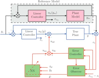
The control scheme under study is depicted on figure 1. A unique linear controller is designed to control the reference model and then applied to the two parallel loops: the reference loop and the complete loop including the whole system, actuators and sensors dynamics. The measured error between these loops is then fed into a compensator
that aims at correcting the linear controller action. The objective is thus to augment the linear control law ulc
with an adaptive element uadso that when applied to the
system, the controlled output y tracks the reference ouput ym. The measured error ym− y is clearly related to the
unmodeled dynamics, so this signal (together with some additional errors, see 1) is treated by the compensator as follows:
• an error observer is designed to extract the unknown dynamics
• a simple neural network computes the extra control signal uadfrom the estimated error and input output
data
As a matter of validation, this control scheme has first been tested on an electromechanical apparatus that represents important classes of ”real life” systems. This test bench represents such physical systems as rigid bodies, flexibil-ity in drive shafts, gearing and belts. The corresponding dynamic model may range from a simple rigid body to a sixth order case with two lightly damped resonances. In that case, the reference model is chosen to cope the rigid body dynamic (order 2), thus neglecting the underdamped
modes. The linear controller is a lead compensator. The results obtained with a 5-neurons 1-hidden layer neural network confirm that this control can cope with the control of simple flexible structures.
The main application treated later is related to the longi-tudinal control of a complete aircraft model of order 193. The reference model (order 7) includes the rigid body dy-namics, the first flexible mode and actuator dynamics. The linear controller is a basic LQR, and the neural network is formed with only 7 neurons on the unique hidden layer. For disturbance rejection scenarii, promising simulation results exhibit a notable decrease in the output signal activity (accelerations, pitch rate, g-load factor).
2. THE ALGORITHM
The global algorithm is represented on figure 1. In the upper loop, the linear controller is associated to the reference model, which is supposed to contain the main dynamic of the real system. Following this idea, main dynamic means that it is known and accurately modeled. On the other hand, the unknown/unmodeled dynamic will be present in the other loop, within the actuator + system transfer. The linear model is designed in a classical way from the knowledge of the reference model. The objective is clearly to use a simple controller with respect to the model complexity. This closed-loop system constitutes the reference model, thus specifying the best performances that should be achieved by the adaptive control process.
The error measured between both control loops is simply
¯ ud ¯ yd ˆ E y ym yc e1 xc unn uad udc ulc(ym) ulc(y) xcm− xc xcm + + + + + + − − − − Linear Controller Linear Controller Error Controller Error Observer True Plant Plant Model Reference Model NN 1
Fig. 1. Adaptive control scheme with reference model the difference between both outputs ym and y. Then the
adaptation signal uadis added to the current control signal
ulc in order to compensate the effects of the unmodeled
dynamics and then to force the lower loop to exhibit the same behavior as the above one. In other words, the idea is to augment the linear control law ulc with an adaptive
element so that when applied to the system, then output y tracks reference output ym. This is achieved by employing
the adaptive control method in [Hovakimyan (2002)]. The adaptation process (lower loop) is composed of different elements with specific tasks:
• the error observer is used to estimate the states of the error dynamics ˆEfrom the output error e1= ym−
y and from the controller state error xcm− xc. This
estimation will be fed into the neural network. • the neural network aims at reconstructing the
sys-tem uncertainty from the estimated error dynamics ˆ
E and from a finite history of available input/output ¯
ud and ¯yd.
• the error controller can be added to accelerate the neural network adaptation and to improve the convergence of the tracking error e1
Considering the closed loop reference model (upper loop on figure 1), the state equations are given by:
˙
Xm= ¯AXm+ ¯Byc (1)
ym= ¯CXm (2)
where yc is the reference signal or setpoint. The state
vector Xm is partitioned sot that XmT = £ χTm zmT xTcm
¤ where χm is the reference model state vector, zm is the
state vector of internal dynamics, and xcm is the linear
controller state vector. In a similar way, and taking into account the control law:
u= ulc− uad (3)
one can write the state equations of the lower loop in a compact form:
˙
X= ¯AX+ ¯Byc− ¯B′uad+ ∆ (4)
y= ¯CX (5)
where X is partitioned so that XT = £ χT zT 1 xTc
¤ with χ being the system state vector, z1 representing
the part of the states of the internal dynamics that are modeled through zm, and xc being the linear controller
state vector. The uncertainties are represented by ∆T =
£ ∆T 1 ∆T2 0
¤
where ∆1 and ∆2 are the matched and
unmatched uncertainties respectively.
As equations (1) and (4) give the current state of the reference loop and the system loop respectively, it is possible to extract the error dynamic by subtracting both equations, leading to:
˙ E= ¯AE+ ¯B′(u ad− ∆1) − B∆2 (6) Z= CE (7) where E≡ Xm− X (8)
is the error dynamic, B and C are matrices of appropriate dimensions, Z represents the signals available for feedback:
Z = · ym− y xcm− xc ¸ (9) Hovakimyan (2002) has demonstrated that ∆1can always
be estimated with an arbitrary accuracy ε∗
using a single hidden layer neural network:
∆1= MTσ(NTη) + ε(η), kε(η)k ≤ ε∗ (10)
where σ(.) is the activation function, M and N are the input and output network weights, ε(η) is the neural network reconstruction error and η is the network input vector (finite history of available input/output data):
η(t) =£ 1 ¯uT
d(t) ¯yTd(t)
¤T
(11) Finally, the adaptive signal uad is designed as:
uad= unn= ˆMTσ( ˆNTη) (12)
The weight adaptation laws are similar to the ones in Hovakimyan (2002). To this, it is needed to estimate error dynamic ˆE. This can be easily performed by the following error observer:
˙ˆ
E= ¯A ˆE+ K(Z − ¯C ˆE) (13) with K chosen so that ¯A− K ¯C is stable and more rapid than ¯A.
3. AIRCRAFT MODEL
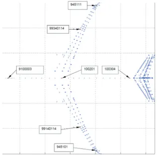
The models used during this work are linear state models corresponding to different Mach numbers and different positions of the center of gravity (depending on fuel tank configurations). There are 7 inputs: 6 command inputs (of which inner aileron IA, outer aileron OA and elevator δ deflections) and 1 disturbance input (wind turbulence). Among the 105 available outputs, some of them are of major interest, like angle of attack α, pitch angle θ and rate q, vertical velocity Vzand acceleration nz. These measures
are made at the center of gravity, but the problem to be treated is clearly related to flexible modes damping, more vertical acceleration measures are needed. On figure 2 are represented the location of the different nz measures.
Fig. 2. Location of the 7 nzmeasures
3.1 Actuators and sensors simulation
Simulation of actuators includes typical nonlinearities like rate limiters and saturations. The bandwidths are approx-imatively 27rd/s for the inner aileron, 10rd/s for the outer aileron and 25rd/s for the elevator.
The measures are simulated using low-pass filters with a 3Hz bandwidth plus a pure delay of 160ms.
Note that the wind turbulence input is simulated using a white noise passing through a Von Karman filter.
3.2 Reduced model
Even if the full order model contains the entire dynamic, the high frequency modes are not considered as essential in the control law design process. In order to reduce the computational burden, a classical order reduction procedure has been used, resulting to model of order 42. Following this idea, the procedure can be continued until reducing the dynamic to its minimum size, i.e. an order 2 corresponding to the rigid body dynamic. On figure 3 are plotted the bode diagrams of the transfer function IA(p)α(p) for the 3 dimensions (193 in blue, 42 in green and 2 in red). Clearly the reduced model is valid up to 50rd/s, which is superior to the desired closed loop bandwidth.
Fig. 3. Bode plots of full order, reduced order and rigid models
3.3 Control objective
The main objective remains the reduction of oscillations produced by either the classical aircraft control or the disturbances (wind gusts and shears). Considering the transfers from wind input to the different nz measures,
it will be asked to reduce as much as possible the main resonant peaks using the inner aileron as control variable. Among the available measures, we will consider more particularly:
• nzCG, vertical acceleration at the aircraft center of
gravity (index 100201 on figure 2), which is directly related to passengers comfort.
• nzL and nzR, vertical accelerations on the left and
right wings (indexes 99140114 and 99340114 on figure 2). These measures give a good feedback of the structure flexibility.
then a combination of these measures will be built, leading to a criterion representing a good trade-off between the passengers feeling due to oscillations and the mechanical energy: the following criterion has been validated:
nzlaw =
nzL+ nzR
4. CONTROL 4.1 Reduced order reference model
The success of the simulation is obviously related to the choice of the reference model. The first idea was to reduce this reference model to its minimal size, i.e. considering the rigid body dynamic and thus discarding the flexible modes, the actuators and sensors dynamics. The resulting model, of order 2, with state vector xm = [ α q ]
T
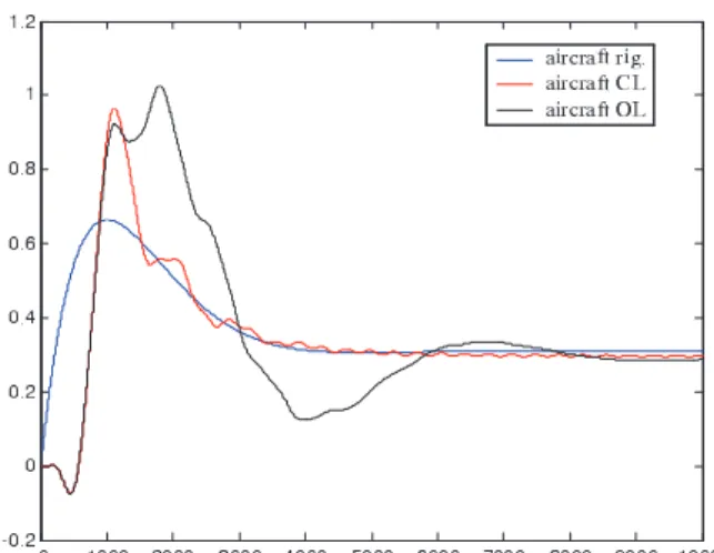
has been combined with a state feedback controller designed to double the damping ratio while keeping the natural frequency. The resulting simulations are not convincing as it can be observed on figures 4 and 5. The simulation corresponds to a tracking problem (step response for α): the blue plot is the output of the reference model (rigid body dynamic of order 2), the red one is the output of the global closed loop model (order 43), and the black plot corresponds to the open loop behavior. Considering first α, the benefit is clear as the output tracks the reference output without exhibiting any flexible modes (fig. 4). On the other hand, the evolution of the pitch rate (fig. 5) is affected by many high frequency modes which are not visible on the open loop dynamic! This phenomenon is also present for any nzmeasure, and of course for nzlaw. Here
this phenomenon is due to spillover: some damping ratios are improved, some others are deteriorated and these mode transitions are not mastered at all. Finally, it appears that there is no way of controlling the whole modes using such a simple reference model (and a simple controller).
Fig. 4. Simulation of the angle of attack α
4.2 More realistic choice for the reference model
The reference model is augmented by adding the first flexible mode (around 1.2Hz) and the actuators dynamic, leading to an order 7. The input variable is still the inner aileron deflection (IA), the available outputs are nzCG,
nzR, nzL, nzlaw, α and q, but only nzlawis considered. The
controller is designed using a LQG strategy by minimizing the following criterion:
Fig. 5. Simulation of the pitch rate q J = ∞ Z 0 (χT mQχm+ Ru2)dt (15)
where χmis the state vector. As the design of the controller
is not the key point, the weighting matrices are not accurately tuned (Q = 5I7 and R = 0.5 in this case).
The resulting controller is
ulc = kcyc− Klqgχm (16)
The neural network is composed of a single hidden layer of 7 neurons. Input/output data history that is fed into the neural network (¯ud and ¯yd) is limited to 19 samples
(sampling period is 2ms). For simplicity reasons, the error observer is not used in that simulation, so that the output error e1 = ym− y is directly fed into the neural network
together with ¯ud and ¯yd. For the same reasons as before,
the error controller is omitted, so that uad= unn(figure 1).
The setpoint is nzCG= 0.1g, so that in steady state nzlaw
Fig. 6. Simulation of the outputs over 10s
should remain null. Simulation results are shown on figure 6: as the open loop evolution of nzlaw is depicted in blue,
ym (green curve) with the controlled output nzlaw (red
curve). First the output error remains weak although both dynamics are clearly different. Indeed, the first flexible mode (around 1.2Hz) is visible on ym (as it belongs to
the reference model) and on nzlaw, but nzlaw also exhibits
higher modes (next one can be measured around 2.7Hz). Then it can be underlined that the transient response of nzlaw is good, including less overshoot than the reference
output.
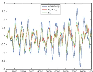
On figure 7 are given the ”classical” control law signal ulc
(red curve) and the effective control signal ulc+uad= ulc+
unn (black curve). Although the difference between both
Fig. 7. Effect of the neural network adaptation
curves is not that obvious, the effect on the output signal nzlaw is clear. That being said, different neural network
tuning would lead to slightly different results: in a classical way, the more sensitive mode is the first flexible mode not belonging to the reference model, i.e. the 2.7Hz mode. One way to improve the efficiency of adaptation is to add an error controller. Here we have chosen a simple lead compensator of transfer function:
Udc(s) = 20
s+ 3
s+ 20E1(s) (17) The simulation setpoint is now zero, that is to say we consider a disturbance rejection problem. Disturbance is simulated using the wind input. Once again, the results presented in figure 8 show an improvement with respect to open loop behavior (green curve). Moreover, the effect of the error compensator through udc allows a reduction
of the nzlaw activity (red curve). As it is quite difficult to
get measurable indexes of the control quality from figure 8 only, it is chosen to build an energy criterion C from the controlled output: C(t) = t Z 0 n2zlawdt (18)
The criterion evolution given on figure 9 confirms the better behavior of the adaptation based on both neural network and error controller. Although the adaptation algorithm has not been detailed in this paper, there are
Fig. 8. nzlaw evolution in case of disturbance rejection
Fig. 9. Evolution of the energy criterion C(t)
many degrees of freedom left to tune the adaptability capabilities of the neural network (see Hovakimyan (2002) and Yang (2004)). This work has shown that it is always possible to find a set of tuning parameters leading to an improvement of the closed loop behavior, this keeping a small sized neural network together with a basic error controller like (17). This last point will become crucial when a real time implementation will be considered.
5. CONCLUSION
Augmenting a linear controller with an adaptive output feedback element based on neural networks is a concept already studied and validated on real-time applications. The open problem treated along this work is the extension to a very high order system composed of many flexible modes. Clearly, it appears that the keypoint is the choice of the ”best” reference model, i.e. getting the optimal balance between simplicity and representability of the main dynamic. The good results obtained during these first steps are encouraging us to come on. More particularly, special effort has to be made to develop a systematic approach for the choice of that reference model.
REFERENCES
B.J. Yang, N. Hovakimyan, A.J. Calise and J.I. Craig. Experimental Validation of an Augmenting Approach to Adaptive Control of Uncertain Nonlinear Systems. AIAA Guidance, Navigation and Control Conference, number AIAA-2003-5715, 2003.
N. Hovakimyan, B.J. Yang, , and A.J. Calise. An Adap-tive Output Feedback Control Methodology for Non-Minimum Phase Systems. Conference on Decision and Control pages 949–954, Las Vegas, 2002.
N. Hovakimyan, F. Nardi, N. Kim, and A.J. Calise. Adap-tive Output Feedback Control of Uncertain Systems using Single Hidden Layer Neural Networks. IEEE, Transactions on Neural Networks, vol.13, n6, Nov. 2002. B.J. Yang. Adaptive Output feedback Control of Flexible Systems. PhD dissertation, School of Aerospace Engi-neering Georgia Institute of Technology, 2004.
M. Jeanneau. Commande Active de Structures Flexibles : Applications Spatiales et A´eronautiques. Lecture notes, Supa´ero, 2000.
Y. Zhang, B. Fidan, and P.A. Ioannou. Backstepping control of Linear Time-Vaying Systems with Known and Unknown Parameters. IEEE, Transactions on Automatic Control, vol.48, n11, Nov. 2003.
L. Bako. Commande adaptative des modes de flexion voilure. MSc dissertation. Ecole Sup´erieure d’Ing´enieurs de Poitiers, 2003.
I.D. Landau. From robust to adaptive control. Control Engineering Practice. vol. 7, pages 1113–1124, 2003.