Pépite | Etude expérimentale et théorique de la capture de radicaux peroxy par la surface d’aérosols organiques

Texte intégral

(1)Thèse de Antoine Roose, Université de Lille, 2019. Ecole Doctorale Science de la Matière, du Rayonnement et de l’Environnement. Thèse de doctorat Présentée par. Antoine ROOSE En vue d’obtenir le titre de Docteur en physique de l’université de Lille. Experimental and theoretical study of the uptake of peroxy radicals by organic aerosol surfaces Etude expérimentale et théorique de la capture de radicaux peroxy par la surface d’aérosols organiques Thèse dirigée par Denis DUFLOT et Véronique RIFFAULT Préparée aux laboratoires PhLAM et SAGE Date de soutenance le 18 décembre 2019 devant le jury d’examen :. Président : Yuri BEDJANIAN – Directeur de recherches CNRS (U. Orléans, ICARE). Rapporteurs : Manuel RUIZ-LOPEZ – Directeur de recherches CNRS (U. Lorraine, LPCT) Barbara NOZIERE – Directrice de recherches CNRS (U. Lyon, IRCELYON). Examinateurs : Delphine VARDANEGA – Maitre de conférences (U. Franche-Comté, UTINAM). Directeur de Thèse : Denis DUFLOT – Maitre de conférences HDR (U. Lille, PhLAM) Co-directrice de Thèse : Véronique RIFFAULT - Professeure (IMT Lille Douai, SAGE). Encadrants : Céline TOUBIN – Professeure (U. Lille, PhLAM) Sébastien DUSANTER – Maitre-Assistant (IMT Lille Douai, SAGE). © 2019 Tous droits réservés.. lilliad.univ-lille.fr.

(2) Thèse de Antoine Roose, Université de Lille, 2019. © 2019 Tous droits réservés.. lilliad.univ-lille.fr.

(3) Thèse de Antoine Roose, Université de Lille, 2019. “They’ve learned to realize that whether they like a theory or they don’t like a theory is not the essential question. Rather, it is whether or not the theory gives predictions that agree with experiment. It is not a question of whether a theory is philosophically delightful, or easy to understand, or perfectly reasonable from the point of view of common sense. […]. So I hope you can accept Nature as She is—absurd.” Richard P. Feynman – QED the strange theory of light and matter. “God made the bulk; surfaces were invented by the devil” Wolfgang Pauli. ii © 2019 Tous droits réservés.. lilliad.univ-lille.fr.


(5) Thèse de Antoine Roose, Université de Lille, 2019. ACKNOWLEDGMENT Je tiens tout d’abord à remercier M. Bedjanian d’avoir accepté de présider ma soutenance de thèse ainsi que Mme. Nozière et M. Ruiz-Lopez d’avoir accepté de lire et évaluer ce manuscrit et enfin, Mme. Vardanega d’avoir examiné mes travaux. Merci pour les discussions scientifiques et les remarques judicieuses apportées lors de la soutenance. Cette thèse a été menée conjointement au sein de deux laboratoires, le laboratoire de Physique des Lasers, Atomes et Molécules ainsi que le laboratoire de Sciences de l’Atmosphère et Génie de l’Environnement. Je tiens donc à remercier Marc Douay et Patrice Coddeville de m’avoir accueilli au sein de leur groupe de recherche. Cette thèse n’aurait pu être ce qu’elle est sans la direction de Denis et Véronique ainsi que la supervision de Céline et Sébastien. Merci à Denis pour ces nombreuses discussions scientifiques ou non, son soutien que ce soit moral, scientifique ou administratif. Merci à Véronique pour tous ses conseils et également pour avoir organisé les rassemblements de ses doctorants et post-doctorants autour de plusieurs repas. Merci à Sébastien pour ses conseils et son soutien tout au long du développement du réacteur. Merci à Céline pour son attention et pour son encadrement qui est toujours efficace. Merci à vous quatre pour m’avoir fait confiance pendant ces 3 ans. Mes travaux expérimentaux n’auraient pas été possibles sans le support de tous les techniciens et ingénieurs de Douai. Je tiens donc à les remercier et tout particulièrement Emmanuel Tison pour son aide pour les réparations du CPC. Je remercie également Florent et Valérie pour la gestion du cluster du PhLAM, vous êtes toujours disponibles pour apporter votre aide, c’est très appréciable. Je remercie également Denis et André pour la gestion des allocations d’heures sur les clusters nationaux. Sans une bonne ambiance de travail, il est plus difficile de mener une thèse à son terme. Je tiens donc à remercier tous mes collègues qui ont participé à cette ambiance qu’ils soient permanents, post-doctorants, doctorants ou stagiaires. Je remercie notamment les habitués du Black night (ils se reconnaitront) avec qui j’ai eu de nombreuses discussions animées. Je remercie également Ahmad, Marius et Asma pour l’ambiance au sein du laboratoire réactivité. Je tiens également à remercier ma famille pour leur soutien tout au long de mes études. Enfin, je remercie Pauline pour son soutien et sa patience tout au long de ces 3 ans. Merci de partager ma vie.. iv © 2019 Tous droits réservés.. lilliad.univ-lille.fr.


(7) Thèse de Antoine Roose, Université de Lille, 2019. Table of contents. TABLE OF CONTENTS Acknowledgment ...................................................................................................................... iv Table of contents ....................................................................................................................... vi List of figures ............................................................................................................................. x List of tables ...........................................................................................................................xvii List of abreviations ................................................................................................................. xix Introduction ................................................................................................................................ 1 Chapter 1: Context and objectives ............................................................................................. 6 I. Chemistry of ROx radicals .................................................................................................. 6 I.1. Radical sources ............................................................................................................ 6. I.2. Radical sinks ............................................................................................................... 8. I.3. Radical chemistry in various areas .............................................................................. 8. I.4. Current understanding of atmospheric ROx chemistry ............................................. 12 Comparison of ROx measurements to atmospheric modeling ........................... 12 Impact of the HO2 uptake on the ROx chemistry ............................................... 14. II. Study of uptake processes................................................................................................. 16 II.1. Theoretical models of uptake .................................................................................... 17 Continuum flux model ....................................................................................... 18 Kinetic resistance model .................................................................................... 18 Kinetic flux model ............................................................................................. 20 Summary ............................................................................................................ 21. II.2. Experimental investigation of HO2 uptake................................................................ 21 Laboratory apparatus ......................................................................................... 21 Dependence of the HO2 uptake on aerosol composition and temperature......... 24 Impact of Relative Humidity (RH) .................................................................... 27 Impact of pH ...................................................................................................... 29 Review of uptake measurements reported in the literature ................................ 30. III. Aerosol simulations at the molecular level ................................................................... 34. III.1. Molecular dynamics (MD) studies ............................................................................ 34. III.2. Quantum Mechanical studies .................................................................................... 37. III.3. Studies investigating the reactivity of HO2 ............................................................... 38. IV. Objectives and strategy ................................................................................................. 42. Chapter 2: Methodology .......................................................................................................... 45. vi © 2019 Tous droits réservés.. lilliad.univ-lille.fr.

(8) Thèse de Antoine Roose, Université de Lille, 2019. Table of contents I. Experimental apparatus for measuring uptake coefficients .............................................. 45 I.1. Aerosol Flow Tube (AFT) design ............................................................................. 45. I.2. Aerosol generation .................................................................................................... 49. I.3. Peroxy radical (HO2, RO2) generation ...................................................................... 51. I.4. Measurements of peroxy radicals - PERCA system ................................................. 52. I.5. Aerosol measurement - Scanning Mobilizer Particle Sizer ...................................... 55. I.6. Uptake measurement procedure ................................................................................ 56. II. Molecular level calculations ............................................................................................. 57 II.1. Molecular dynamics .................................................................................................. 58 Principle ............................................................................................................. 58 Force fields......................................................................................................... 62. II.2. Quantum chemistry ................................................................................................... 63 Schrödinger equation and Born-Oppenheimer approximation .......................... 64 Computational methods ..................................................................................... 65 The ONIOM method .......................................................................................... 72 Conclusion on the quantum mechanics methods ............................................... 73. II.3. Treatment of reactivity .............................................................................................. 74 Transition State Theory...................................................................................... 74 Activated complex theory .................................................................................. 75. II.4. Analysis methods ...................................................................................................... 77 Binding energy ................................................................................................... 77 Radial distribution function ............................................................................... 78 Connolly surface ................................................................................................ 78 Autocorrelation function .................................................................................... 79. Chapter 3: Characterization of the aerosol flow tube and development of a methodology for HO2 uptake measurements ....................................................................................................... 80 I. Characterization of the AFT ............................................................................................. 80 I.1. Parameterization of the radical-aerosol contact time ................................................ 80. I.2. Characterization of the two aerosol generation setups .............................................. 84 Nebulization setup ............................................................................................. 85. Dependence of the aerosol size distribution on the glutaric acid concentration in solution 87 Nucleation setup................................................................................................. 90 Conclusions on aerosol generation .................................................................... 93 I.3. Characterization of aerosol wall losses in the AFT................................................... 94 vii. © 2019 Tous droits réservés.. lilliad.univ-lille.fr.

(9) Thèse de Antoine Roose, Université de Lille, 2019. Table of contents I.4. Characterization of the HO2 radical source ............................................................... 98. I.5. Characterization of HO2 wall losses in the AFT and gas-phase losses from HO2+HO2 100. II. Uptake measurements ..................................................................................................... 104 II.1. Development of a measurement procedure ............................................................. 104 Measurement of the HO2 decay ....................................................................... 104 Determination of the HO2 loss rate due to aerosol uptake ............................... 106 Determination of the HO2 uptake coefficient .................................................. 108. II.2. Measurements of HO2 uptakes on glutaric acid aerosols and dependence on RH .. 109. Chapter 4: Molecular modelling of the HO2 uptake .............................................................. 111 I. Benchmarking of the force field ..................................................................................... 111 I.1. Monomer of glutaric acid ........................................................................................ 111. I.2. Glutaric acid-glutaric acid interactions ................................................................... 118. I.3. Clusters of glutaric acid and water .......................................................................... 122. I.4. Valeric acid ............................................................................................................. 123. II. Aerosol formation ........................................................................................................... 125 II.1. Adjustment of the minimum box size ..................................................................... 125. II.2. Methodological approach ........................................................................................ 126 Dry aggregate ................................................................................................... 126 Wet aerosol ...................................................................................................... 129. II.3. Aerosol characterization .......................................................................................... 130 Impact of the methodology on the stability ..................................................... 130 ACS Earth and Space Chemistry paper ........................................................... 134 Experimental considerations ............................................................................ 145. III. HO2 mass accommodation coefficient computation ................................................... 146. III.1. All in one approach ................................................................................................. 146. III.2. Statistical approach ................................................................................................. 151. IV. Computation of the reactivity ..................................................................................... 155. IV.1 Gas phase reactivity ................................................................................................ 155 IV.2 Aerosol surface reactivity........................................................................................ 158 CONCLUSION ...................................................................................................................... 162 I. Conclusion and perspectives of the experimental part ................................................... 162 I.1. Conclusions ............................................................................................................. 162. I.2. Perspectives ............................................................................................................. 163. II. Conclusions and perspectives of the theoretical part...................................................... 164 viii. © 2019 Tous droits réservés.. lilliad.univ-lille.fr.

(10) Thèse de Antoine Roose, Université de Lille, 2019. Table of contents II.1. Conclusions ............................................................................................................. 164. II.2. Perspectives ............................................................................................................. 165. REFERENCES ...................................................................................................................... 166 APPENDICES ....................................................................................................................... 192 ABSTRACT ........................................................................................................................... 208. ix © 2019 Tous droits réservés.. lilliad.univ-lille.fr.

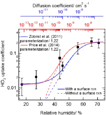
(11) Thèse de Antoine Roose, Université de Lille, 2019. List of figures. LIST OF FIGURES Figure 1: Layers of the atmosphere.2 ......................................................................................... 2 Figure 2: Schematic of chemical and transport processes related to atmospheric composition 7 .................................................................................................................................................... 3 Figure 3: Radiative forcing for the period 1750-2011.11 ........................................................... 4 Figure 4: Pie charts showing the average diurnal modeled OH and HO2 sources and sinks between 12:00 and 13:00 over the tropical Atlantic ocean. Figure taken from Whalley et al. (2010)24 ...................................................................................................................................... 9 Figure 5: Chemical reaction scheme showing the reactions affecting OH and HO 2 concentrations. X=I, Br and R= alkyl group. Figure taken from Whalley et al. (2010) 24 ...... 10 Figure 6: Daytime average ROx budget at Tung Chung (China) on 25 August 2011. The unit is ppb h-1. The red, blue and green lines indicate the initiation, termination and propagation pathways of radicals, respectively.29........................................................................................ 11 Figure 7: HOx budget in a boreal forest. Radical production (green), recycling (blue), and loss (red) pathways are indicated by bold arrows. All rates are given in 106 molecule cm-3 s-1.13 . 12 Figure 8: Diurnal cycle of HO2 between 20 June and 30 July 2009 during the BEARPEX09 field campaign. Modeled HO2 concentration is represented in red and observed HO2 concentration is represented in blue. The interferences coming from FAGE are marked by the shaded area.34 ........................................................................................................................... 13 Figure 9: Impact on the annual mean concentrations of oxidants and sulfur species when moving from a γ(HO2) value of 0.2 (Jacob,2000)35 to the scheme presented in Table 1 (global mean γ(HO2) of 0.028)36 .......................................................................................................... 16 Figure 10: Schematic of the processes that govern heterogeneous radical uptake by aerosol particles.79 ................................................................................................................................ 17 Figure 11: a) Resistor model for an uptake limited by gas-phase diffusion, mass accommodation, and solubility. b) Resistor model for an uptake limited by gas-phase diffusion, mass accommodation, solubility, liquid-phase reaction and surface reaction.72 ..................... 19 Figure 12: Kinetic multi-layer model (KM-SUB): (a) Model compartments and layers with corresponding distances from particle center (rp ± x), surface area (A) and volumes (V); λXi is the mean free path of Xi in the gas-phase; δXi and δYj are the thickness of sorption and quasistatic bulk layers, respectively; δ is the bulk layer thickness. (b) Transport fluxes (green arrows) and chemical reactions (red arrows).83..................................................................................... 21 Figure 13: Different types of reactors to study gas-aerosol interactions. A) Knudsen cell reactor;87 B) Droplet flow reactor;88 C) Aerosol Flow tube reactor;89 D) Cloud chamber system;90 E) Wall coated flow tube91 ....................................................................................... 24 Figure 14: Measurements of HO2 uptake on organic particles.51–54 These measurements were performed by the Research Institute for Global Change of the Japan Agency for Marine-earth Science and Technology in Yokohoma (red) and by the School of Chemistry, of the University of Leeds, England (blue). ......................................................................................................... 25 Figure 15: Summary of laboratory data for γHO2 plotted as a function of temperature. Filled symbols denote that the aerosol was doped with Cu. Colors refer to composition as follows: red, sulfur-containing aerosols; green, Cl- (or Br-) containing salts, i.e. sea salt; black, soot; yellow, ammonium nitrate; blue, water. Solid lines indicate temperature dependencies for NH4NO3 (Gershenzon et al., 199993), and for solid NaCl (Remorov et al., 200263), respectively. x © 2019 Tous droits réservés.. lilliad.univ-lille.fr.

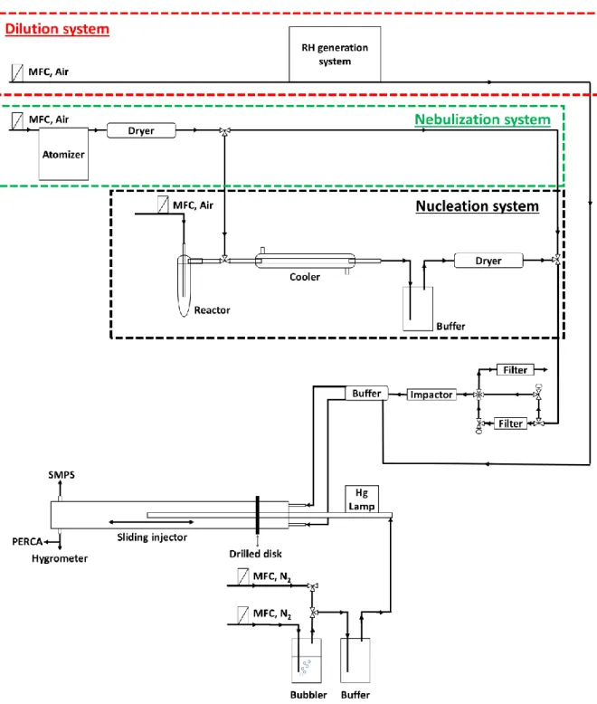
(12) Thèse de Antoine Roose, Université de Lille, 2019. List of figures Error bars as quoted in the references and arrows indicate greater than or less than. The red dot-dash line indicates the temperature dependence of the parameterization assumed in Macintyre and Evans, 201136 (assuming 50% of relative humidity). The black dotted line indicates a value of 0.2, as recommended by Jacob (2000)35, and the dashed black line reports the parameterization of Thornton et al. (2008)42 (assuming pH = 5, r = 100 nm, α = 1, [HO2] = 108 cm-3), used by Mao et al. (2010)92 to fit model based on laboratory data with ARCTAS observation. Letters indicate references as follows: a Mozurkewich et al., 1987,62 b Hanson et al., 1992,43 c Gershenzon et al., 1995,59 d Cooper and Abbatt, 1996,44 e Gershenzon et al., 1999,93 f Thornton and Abbatt, 2005,94 g Taketani et al., 2008,68 h Taketani et al., 2009,67 i Loukhovitskaya et al., 2009,60 j Bedjanian et al., 2005,55 k Saathoff et al., 2001.64 Figure taken from Macintyre and Evans, 201136. ......................................................................................... 26 Figure 16: HO2 uptake coefficient as a function of the estimated Cu(II) molality for ammonium sulfate aerosols at 65 % RH and 293 ± 2 K. The error bars are 2 standard deviations. Red line: fitting of 1/γ = 1/α + 1/(A.[Cu]) with α = 0.26 and A = 197 L mol-1. Blue line: fitting of 1/γ = 1/0.26 + 1/(B.[Cu]0.5) where B = 1.8 (mol L)-(1/2). Figure taken from Matthews 2014, experimental data obtained by Dr. Ingrid George.95 ................................................................ 27 Figure 17: Influence of RH on the HO2 uptake for Arizona Test Dust.56,61 ............................ 28 Figure 18: HO2 uptake coefficient onto Cu(II)-doped sucrose aerosol particles as a function of relative humidity. Figure taken from Lakey et al.52 ................................................................. 29 Figure 19: Theoretical HO2 uptake coefficient as a function of aerosol pH for an aerosol radius of 100 nm, a temperature of 293 K and a HO2 concentration of 5 × 108 molecule cm-3. Figure taken from Matthews 95 ............................................................................................................ 30 Figure 20: Equilibrium snapshots of formic acid aggregates at 100, 150 and 200 K (left, middle, and right) and for 0, 50, 66, and 83 mol. % water concentrations (from top to bottom) (Vardanega et al. 2014).115 ....................................................................................................... 35 Figure 21: A) Schematic of MD scattering simulation; B) Calculated density profile of the liquid film of water (Motsuoka –Clementi-Yoshimine model of water); C and D) Two examples of MD scattering trajectories during 20ps. The solid lines denote the Z coordinates of water molecules, and the dashed lines with the label “ho2” denote two HO2 radicals scattering onto the liquid water surface. Note that the solid region in -20Å<Z<20Å corresponds to the slab of water.119 .............................................................................................................. 36 Figure 22: Optimized B3LYP/aug-cc-pVDZ dicarboxylic acid H2DCn (n = 0-12) structures.124 .................................................................................................................................................. 38 Figure 23: HO2.H2O equilibrium constant as a function of temperature. Keq is in units of cm3 molecule-1 taken from Aloisio and Francisco.125 ..................................................................... 39 Figure 24: Reaction model of electron capture of HOO on ice taken from Tachikawa .128 .... 40 Figure 25: Unconstrained 50 ps MD simulations with the radicals initially placed at the airwater interface. Left: Snapshot at the end of the simulation showing HO 2 at the air-water interface (upper) and O2- in bulk water (lower). Right: Density profiles for the radicals and water (X=0 corresponds to the center of the simulation box or the water slab) taken from Martins-Costa et al.130 .............................................................................................................. 41 Figure 26: Comparison of dicarboxylic acids distribution in urban/continental and remote marine areas7 ............................................................................................................................ 43 Figure 27: Schematic of the Aerosol Flow tube constructed in the SAGE department. ......... 46 Figure 28: Schematic of the whole AFT setup (MFC: Mass flow controller). The impactor used has a 0.071 cm diameter nozzle. .............................................................................................. 47 xi © 2019 Tous droits réservés.. lilliad.univ-lille.fr.

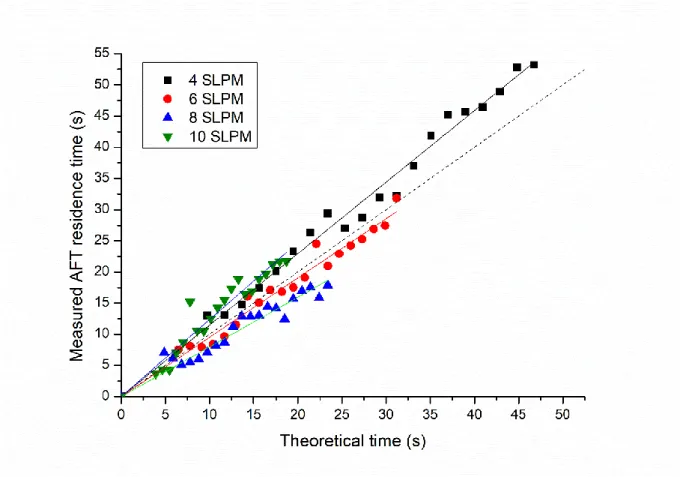
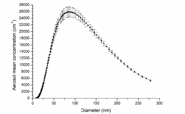
(13) Thèse de Antoine Roose, Université de Lille, 2019. List of figures Figure 29: Picture of the AFT setup. ....................................................................................... 48 Figure 30: Schematic of the velocity gradient for laminar flow conditions. ........................... 49 Figure 31: Schematic of the nebulizer (left) and the denuder (right).144 ................................. 50 Figure 32: Picture (left) and schematic (right) of the aerosol generation setup based on the nucleation of organic vapors. Red and black lines represent the heating wires that are controlled by both temperature controller. ................................................................................................ 51 Figure 33: Schematic of the peroxy radical generation system. .............................................. 51 Figure 34: Dependence of experimental (blue, left y-axis) and modeled (red, right y-axis) CL on RH for the ECHAMP and PERCA approaches (T = 23±2°C). The filled diamond represents calibration experiments performed in the field. Error bars are 3σ standard errors. Figure taken from Duncianu et al. ................................................................................................................ 54 Figure 35: Schematic (left) and picture (right) of the PERCA setup described in Duncianu et al. (2019 in review)153. SV accounts for Solenoid Valve, CAPS for Cavity Attenuated Phase Shift spectroscopy and PFA for Perfluoroalkoxy. ................................................................... 54 Figure 36: Schematics of the DMA (left) and CPC (right). ..................................................... 56 Figure 37: Scheme of the leap-frog integrator with x the position and v the velocity.157 ....... 58 Figure 38: Illustration of the fundamental force field terms.161 ............................................... 60 Figure 39: Definition of the improper angle.161 ....................................................................... 60 Figure 40: Illustration of the boxes and the application of periodic boundary conditions. All the interaction are computed within the radius of the Rc (represented by the red dotted circle). Figure taken from Fotsing164.................................................................................................... 61 Figure 41: Typical time and length scales of different simulation techniques: quantum mechanics (QM), including coupled cluster (CC) and Density Functional Theory (DFT) methods (see below); molecular mechanics (MM) including all-atom molecular dynamics (AA-MD) simulations, implicit solvent and coarse grained MD (IS-MD and CG-MD), and Brownian dynamics (BD) technique; and continuum mechanics (CM). The ranges of time and length are approximate. Figure taken from OzboyacuI et al. 168 ............................................. 62 Figure 42: A 1s-STO orbital modelled by a linear combination of three GTOs (STO-3G).161 .................................................................................................................................................. 67 Figure 43: The molecular orbital (MO) formed by the interaction between the antisymmetric combination of H 1s orbital and the oxygen px orbital. Bonding interactions are enhanced by mixing a small amount of O dxz character into the MO.182 ...................................................... 68 Figure 44: Correlation contributions for a HF molecule in the cc-pVTZ-(f/d) (white) and augcc-pVDZ (black) basis sets.183 ................................................................................................. 70 Figure 45: Substractive QM/MM coupling as implemented in ONIOM.190............................ 73 Figure 46: Schematic of a reaction path (case of isomerization of ozone).161 ......................... 75 Figure 47: Contour plot illustration of the tunneling path161,197 .............................................. 77 Figure 48: Construction of a radial distribution function199 .................................................... 78 Figure 49: Schematic for the probing of a Connolly surface or solvent accessible surface.20179 Figure 50: Experimental setup used to parameterize the radical-aerosol contact time as a function of the injector position.. ............................................................................................. 81 Figure 51: Residence time of a toluene pulse inside the injector and the AFT measured by PTR-ToFMS for a total flow rate of 6 SLPM. ......................................................................... 82 Figure 52: Plot of the contact time vs the injector position for various total flow rates in the AFT. ......................................................................................................................................... 83. xii © 2019 Tous droits réservés.. lilliad.univ-lille.fr.

(14) Thèse de Antoine Roose, Université de Lille, 2019. List of figures Figure 53: Scatter plot of measured AFT residence times vs. calculated residence times (assuming plug-flow conditions). The dashed line corresponds to the 1:1 line....................... 83 Figure 54: Peak distribution of toluene pulses over different positions of the injector for an AFT flow rate of 6 SLPM. The time indicated on the x-axis is the measurement time from the PTR-ToFMS and is not related to the residence time in the AFT. .......................................... 84 Figure 55: Experimental setup for generating aerosols by nebulization of a liquid solution . 85 Figure 56: Concentration of aerosols generated by nebulization of a 5×10-3 M glutaric acid solution at 3 entrance pressures in the atomizer. Error bar are 3σ ........................................... 86 Figure 57: Glutaric acid aerosols size distribution in SMPS mode at various entrance pressures in the atomizer. Glutaric acid concentration of 5 × 10-3 M...................................................... 87 Figure 58: Size distribution of glutaric acid aerosols formed by atomization of a 5 × 10-3 M glutaric acid solution. Error bars are 1σ standard deviation over two hours of experiment. ... 88 Figure 59: Stability of glutaric acid aerosols formed by atomization of a 5 × 10-3 M glutaric acid solution over two hours of experiment for three size bins in SMPS mode. ..................... 88 Figure 60: Aerosol size distribution for various glutaric acid concentrations (mol L-1) in solution for an entrance pressure of 1 bar in the atomizer. Error bars are 3σ. ......................... 89 Figure 61: schematic of the nucleation setup for aerosol generation. ...................................... 90 Figure 62: a) Total concentration of glutaric acid aerosols generated by nucleation vs. upper (Tup) and lower (Tlow) reactor temperatures, b) particle mean diameter, c) particle geometric diameter, d) examples of size distributions produced for different set of temperatures, e) Comparison of size distributions observed using a backward (magenta) and a forward (green) water flow for the cooling system. Error bars are 3σ. ............................................................. 92 Figure 63: Comparison of surface distributions generated by the nebulization and nucleation setups for glutaric acid aerosols ............................................................................................... 94 Figure 64: AFT setup used for the determination of aerosol wall losses. ................................ 95 Figure 65: Decays of aerosol number concentration (whole distribution) in the AFT. The yellow area represents the area suitable for uptake experiment. ............................................. 96 Figure 66: : Plot of aerosol first-order wall loss rates vs. aerosol size bins. ............................ 97 Figure 67: Plot of parameters a and b from Equation 105 vs. the total surface concentration at position 0 cm. The error bar are 1σ. ......................................................................................... 98 Figure 68: Picture of the quartz cell connected at the upstream end of the injector. The mercury lamp was placed outside the cell and covered with aluminum foil to protect the user from UV radiations. ................................................................................................................................. 99 Figure 69: Concentration of HO2 measured in the AFT vs. water mixing ratio in the injector. ................................................................................................................................................ 100 Figure 70: Picture of the AFT whose inner surface has been coated with halocarbon wax. . 101 Figure 71: Characterization of HO2 wall losses in the AFT – Temporal decays of HO2 (markers: experimental data; lines: linear least-square fits) for the determination of first-order loss rates at different values of relative humidity: 0% (black and gray); 30-33% (red and magenta); 6566% (dark and light blue). Decays for uncoated walls are displayed with square markers while decays for wax coated walls are displayed with triangle. ...................................................... 102 Figure 72: PERCA measurements of HO2 during an uptake experiment for glutaric acid aerosols at 29.7% RH. NO2 concentrations measured under amplification and background conditions by the two CAPS monitors during an uptake experiment. Concentrations lower than 4 ppb were measured by the background channel and concentrations higher than 4 ppb by the. xiii © 2019 Tous droits réservés.. lilliad.univ-lille.fr.

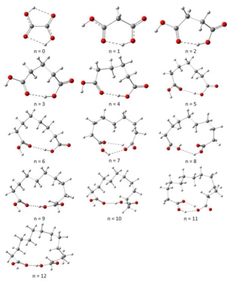
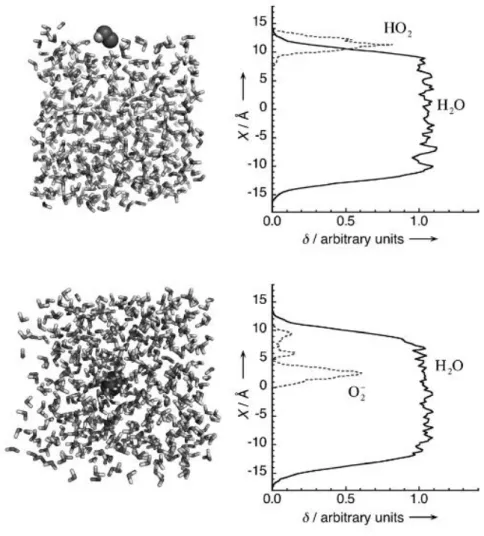
(15) Thèse de Antoine Roose, Université de Lille, 2019. List of figures amplification channel, with the exception of the black symbols (upper panel) displaying the period when both the two channels ran under background conditions (see text). ................. 105 Figure 73: Determination of HO2 loss rates without (wall losses) and with (wall losses+aerosol uptake) aerosols in the AFT for glutaric acid aerosols at 29.7% RH and a total surface concentration of 3.9 cm2 cm-3 - Line: linear least-square fit of the logarithm of HO2 concentrations vs. contact time. Error bars represent 1σ standard deviation. ........................ 106 Figure 74: Determination of the HO2 uptake coefficient for glutaric acid aerosols at 29.7% RH. Line: linear least-square fit of the HO2 first-order loss rate due to aerosol uptake vs. aerosol surface concentration. Error bars represent 1σ standard deviation. ....................................... 108 Figure 75: Scheme representing the glutaric acid molecule. ................................................. 111 Figure 76: Glutaric acid with labeled atoms .......................................................................... 113 Figure 77: Radial distribution of the distance separating the two acid carbons (C7-C8) averaged over the last 5 ns of a 10 ns molecular dynamics simulation of the monomer with AMBER GAFF at 300 K....................................................................................................................... 114 Figure 78: Molecular representation of the three conformers identified for the glutaric acid monomer and the corresponding C7-C8 distances. ............................................................... 114 Figure 79: Variation of the RESP charges for the three conformers as a function of the atom. (Values are in Appendix F) .................................................................................................... 115 Figure 80: Variation of the probability of occurrence of the three conformers as a function of the fudge factor on the Coulomb 1-4 interaction. .................................................................. 117 Figure 81: Scan of the potential energy along the HOCO dihedral angle at MP2/aug-cc-pVDZ. ................................................................................................................................................ 117 Figure 82: Dimers of glutaric acids (GLU)2, dashed lines represent intermolecular H-bonds (in Å ). .......................................................................................................................................... 118 Figure 83: Binding energy distributions for (GLU)2 and (GLU)4 .......................................... 119 Figure 84: Evolution of the C7-C8 radial distribution function with the number of molecules in the cluster. .......................................................................................................................... 120 Figure 85: Structure of the glutaric acid crystal (120 molecules). ......................................... 121 Figure 86: Cluster of one glutaric acid and one water molecules. ......................................... 122 Figure 87: Binding energy distribution of the glutaric acid – water cluster. ......................... 122 Figure 88: Valeric acid dimer minimum energy configuration obtained from ab initio (MP2/6311++G(2d,2p)+ZPE). Bond lengths indicated in Angstroms. ............................................. 123 Figure 89: Valeric acid crystal. .............................................................................................. 124 Figure 90: Radial distribution function of a (GLU)100 aerosol with different box sizes........ 125 Figure 91: A) (GLU)100 in a box of 3.5 nm long after a 10 ns trajectory.; B) (GLU)100 in a box of 20 nm long after a 10 ns trajectory (GAFF). ..................................................................... 126 Figure 92: “One in all” method to form an aerosol of glutaric acid (200 molecules). The molecules are placed randomly in the box followed by a MD run in the NVT ensemble (300K) until stabilization of the potential energy (at least 10 ns). ..................................................... 127 Figure 93: Time evolution of the potential energy showing that the aerosol breaks into two parts or forms again a single particle. .................................................................................... 128 Figure 94: A) (GLU)200 during breaking; B) Two aerosol parts of (GLU)200 before they collide. ................................................................................................................................................ 128 Figure 95: Generation method of wet aggregates by nucleation of water around the dry aggregate. ............................................................................................................................... 130. xiv © 2019 Tous droits réservés.. lilliad.univ-lille.fr.

(16) Thèse de Antoine Roose, Université de Lille, 2019. List of figures Figure 96: Generation method of wet aggregates by cocondensation of both acid and water molecules. .............................................................................................................................. 130 Figure 97: a) Radius of valeric acid aerosols (VA) as a function of the number of molecules N for the different generation processes (GP1: Random generation (Black); GP2: Random generation + annealing (Red); GP3: Random generation + Angular (Blue); GP4: Generation step by step (Pink)). b) Radius of Glutaric acid aerosols (GA) as function of the number of molecules N for the different generation processes. For both figures, the average for a given aerosol size over the generation processes is represented in green. ...................................... 131 Figure 98: Atom surface repartition of (a) the glutaric acid and (b) the valeric acid aggregates made of 50 molecules as a function of the generation process used. .................................... 132 Figure 99: Comparison of the radial distribution functions (RDFs) between the 1:1 ratios of glutaric acid:water aggregates of 100 glutaric acid molecules generated either by cocondensation (Co) method or by nucleation of water on the dry aggregate .......................... 133 Figure 100: Comparison of the atoms repartition at the surface of the glutaric acid aggregate (GA) of 100 molecules (black), the wetted glutaric acid aggregates with a 1:1 glutaric acid:water ratio generated by nucleation of water on the dry aggregate (WA, in red) and by cocondensation (Co, in blue). .................................................................................................... 134 Figure 101: Front cover of the ACS Earth and Space Chemistry issue of March 2019. ....... 135 Figure 102: Computational method used for the mass accommodation coefficient of HO2 (green spheres) on a wetted aggregate, water molecules being represented in blue. ............. 147 Figure 103: Time evolution of the number of gas phase HO2 molecules. ............................. 147 Figure 104: Time evolution of the HO2 concentration in the gas phase determined by the radius method (green), and the gas phase (black), bulk (blue) and surface (red) concentrations determined by the Connolly method. ..................................................................................... 148 Figure 105: Time evolution of the bulk/surface ratio of HO2 molecules .............................. 149 Figure 106: Time evolution of the HO2-glutaric acid (GA, black) and HO2-water (H2O, red) binding energy. ...................................................................................................................... 150 Figure 107: Radial distribution functions of glutaric acid (black), water (blue) and HO2 (red) with respect to the aerosol center of mass. ............................................................................ 150 Figure 108: Snapshots of a) O-acceptor HO2 orientation on a water site, b) H-donor HO2 orientation on a water site, c) O-acceptor HO2 conformation on glutaric acid and d) H -donor HO2 conformation on glutaric acid. The HO2 and the molecule at the adsorption site are represented by spheres, other water molecules in blue spheres and lines and glutaric acid in lines. ....................................................................................................................................... 152 Figure 109: Time evolution of the radial distribution function of HO2, water and glutaric acid (GA) averaged over all trajectories ........................................................................................ 153 Figure 110: Time evolution of the average interactions HO2 - system, HO2 - glutaric acid (GA) and HO2 – water. .................................................................................................................... 154 Figure 111: Snapshot of the two most abundant conformers. The hydrogens with different environment (according to the molecule symmetry) are numbered. ..................................... 155 Figure 112: Potential energy diagram of each reaction way found with both functionals. Values are shown in Appendix H. ..................................................................................................... 156 Figure 113: Geometries of the transition states. The arrows represent the mass weighted imaginary mode. .................................................................................................................... 156 Figure 114: Picture of the transition state (middle) corresponding to a proton exchange. .... 161. xv © 2019 Tous droits réservés.. lilliad.univ-lille.fr.

(17) Thèse de Antoine Roose, Université de Lille, 2019. List of figures Figure 115: A) Double-layer surface model compartments and transport fluxes for the trace gas Xi (left) and non-volatile species Yj (right) B) Classification of chemical reactions between volatile and non-volatile species at the surface.82 .................................................................. 194 Figure 116: Kinetic multi-layer model (KM-SUB): (a) Model compartments and layers with corresponding distances from particle center (rp ± x), surface area (A) and volumes (V); λXi is the mean free path of Xi in the gas-phase; δxi and δYj are the thicknesses of sorption and quasistatic bulk layers; δ is the bulk layer thickness. (b) Transport fluxes (green arrows) and chemical reactions (red arrows).83 ......................................................................................... 196 Figure 117: Size distribution of aerosols generated by atomization of a 5×10-3M glutaric acid solution (black); a 5×10-3M copper sulfate solution (red); a 1:20 Cu/Glutaric acid solution (blue), a solution made of 5×10-3M glutaric acid and 5×10-3M copper sulfate (magenta) a solution made of 5×10-3M glutaric acid and 5×10-3M copper sulfate (green). ...................... 198 Figure 118: Geometries of the reactive Van der Waals complexes (RC) and product Van der Waals complex (PC) of the four different hydrogen environments. ...................................... 204. xvi © 2019 Tous droits réservés.. lilliad.univ-lille.fr.

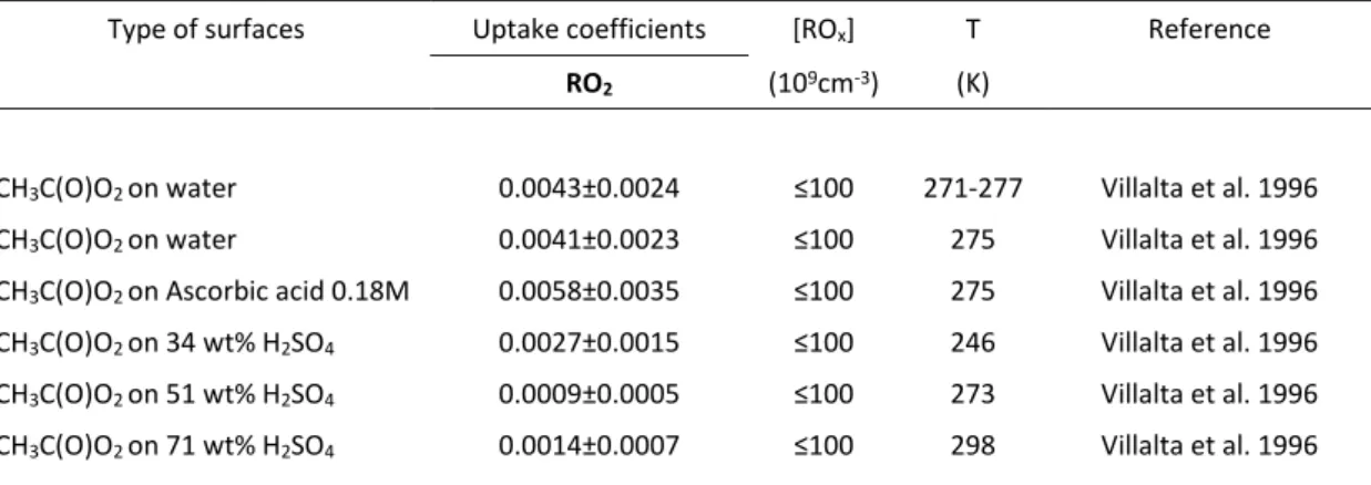
(18) Thèse de Antoine Roose, Université de Lille, 2019. List of tables. LIST OF TABLES Table 1: Uptake coefficients for HO2 used in the Macintyre and Evans (2011) study36 ......... 15 Table 2: Value of HO2 uptake onto glutaric acid found in the literature51,54 ........................... 27 Table 3: Summary of HO2 uptake coefﬁcients for dicarboxylic acids and their dependence on RH at room temperature (from Taketani et al.54)..................................................................... 28 Table 4: Uptake values for inorganic particles and surfaces43,44,56,58,60,61,63,67,68,94,96–99 ........... 31 Table 5: Uptake values for organic particles and surfaces51,52,54,66,98–105 ................................. 32 Table 6: Uptake values for mixed inorganic and organic particles.53 ...................................... 33 Table 7: Efficiency of the diffusion dryer.144........................................................................... 50 Table 8: Specifications of different analytical tools for the quantification of peroxy radicals. .................................................................................................................................................. 52 Table 9: Characteristics of both classifiers used. ..................................................................... 55 Table 10: Characteristics of both condensation particle counters used. .................................. 56 Table 11: Terms of equations 29 - 33. ..................................................................................... 59 Table 12: Comparison of some of the common models used for water 172–175 ........................ 63 Table 13: Summary of the different methods used in quantum mechanics ............................. 73 Table 14: Partition functions for molecular degrees of freedom.194 ........................................ 76 Table 15: parameters of Equation 105 determined for different total aerosol surface concentrations. ......................................................................................................................... 97 Table 16: HO2 wall loss rates as function of humidity and wall coating. .............................. 102 Table 17: HO2 self-reaction contribution to the overall loss rate at different relative humidities in the AFT. ............................................................................................................................. 103 Table 18: Values measured and determined during the uptake measurement at 29.7% RH. 107 Table 19: Operating conditions used during uptake measurements ...................................... 109 Table 20: HO2 uptake coefficient measured on glutaric acid aerosols. Uncertainties have been computed using error propagations. ....................................................................................... 109 Table 21: Details of the energy contributions (kJ mol-1) for a glutaric acid monomer at 300 K with the OPLS/AA FF compared to GAFF. .......................................................................... 112 Table 22: 1-4 Coulomb energy (kJ mol-1) for each interaction pair. ..................................... 113 Table 23: Comparison of the energy differences (kJ mol-1) computed by Energy Minimization (EM) with molecular dynamics (GAFF) and with different quantum methods and basis sets (with ZPE energies). Conformer 1 is taken as the reference. ................................................ 116 Table 24: Comparison of the energy differences (kJ mol-1) along the scan of the potential energy from QM calculations (MP2/aug-cc-pVDZ with ZPE) and MD calculations (GAFF with fudge factor equal to 0.833). .................................................................................................. 118 Table 25: Comparison between the energies of the glutaric acid dimer computed by molecular dynamic and ab initio MP2/6-311++G(2d,2p) method. ........................................................ 119 Table 26: Calculated MD lattice parameters of a glutaric acid crystal (using isotropic pressure and temperature Berendsen couplings) compared to previous works. .................................. 121 Table 27: Binding energies (kJ mol-1) of the valeric acid dimer and valeric acid – water dimer computed by ab initio method and molecular dynamics. ...................................................... 123 Table 28: Calculated MD lattice parameters of valeric acid crystal (using Berendsen isotropic pressure and V-rescale temperature couplings) compared to previous works. ...................... 124 Table 29: Stability of the glutaric and valeric acid aggregates as a function of the number of molecules and the generation process used. ‘-‘: cases not tested. ......................................... 131 xvii © 2019 Tous droits réservés.. lilliad.univ-lille.fr.

(19) Thèse de Antoine Roose, Université de Lille, 2019. List of tables Table 30: Stability of the wetted glutaric acid aggregates formed by co-condensation as a function of the number of molecules, the glutaric acid:water ratio and the generation process used. ‘-‘: cases not tested.. ..................................................................................................... 133 Table 31: Proportion of the adsorption site types (water or glutaric acid (GA)) at the moment when the collision happens (tcollision) and at the end of the simulation (t500ps). The average collision time is about 13.9 ± 5.9 ps. ..................................................................................... 151 Table 32: Summary of the rate constants computed using the transition state theory for both functionnals ............................................................................................................................ 157 Table 33: Summary of the rate constant taking into account the equilibrium constant of the reactive complex formation for both functionals. .................................................................. 158 Table 34: Computations carried out for the deprotonation of HO2 ....................................... 159 Table 35: Computations carried out for the H-abstraction by HO2 ....................................... 160 Table 36: Computation ongoing for the HO2 deprotonation ................................................. 160 Table 37: The atomic unit system. 241 .................................................................................... 197 Table 38: Geometrical parameters used for water and carboxylic acids (glutaric and valeric). Bond distances are given in Ångströms and angles in degrees. ............................................ 200 Table 39: Parameters used for the coulombic interaction potential and the 12-6 Lennard-Jones potential.................................................................................................................................. 201 Table 40: RESP charges (MP2/6-31+G**) of the three glutaric acids conformers. .............. 202 Table 41: HO2 parameters. ..................................................................................................... 203 Table 42: Energies (in kcal mol-1) of the Van der Waals complexes of the glutaric acid Habstraction by HO2. ................................................................................................................ 205. xviii © 2019 Tous droits réservés.. lilliad.univ-lille.fr.

(20) Thèse de Antoine Roose, Université de Lille, 2019. List of abreviations. LIST OF ABREVIATIONS AA-MD: All Atom Molecular Dynamics ACS: American Chemical Society AFT: Aerosol Flow Tube AIMD: Ab Initio Molecular Dynamics AMBER: Assisted Model Building with Energy Refinement AO: Atomic Orbital AU: Atomic Units BD: Brownian Dynamics BEARPEX: Biosphere Effects on Aerosol and Photochemistry Experiment BVOC: Biogenic Volatile Organic Compounds CABINEX: Community Atmosphere Biosphere Interactions Experiment CAPS: Cavity Attenuated Phase Shift CC: Coupled Cluster CCD: Coupled Cluster Doubles CCN : Cloud Condensation Nuclei CCSD: Coupled Cluster Single and Doubles CCSDT: Coupled Cluster Single, Doubles and Triples CCSD(T): Coupled Cluster Single, Doubles with Triples treated perturbatively CG-MD: Coarse Grain Molecular Dynamics CHARMM: Chemistry at HARvard Macromolecular Mechanics CIMS: Chemical Ionization Mass Spectrometry CL: Chain Length CM: Continuum Mechanics COM: Center Of Mass CPC: Condensation Particle Counter CPU: Central Processing Unit DFT: Density Functional Theory DFTB: Density Functional Tight Binding DMA: Differential Mobility Analyzer xix © 2019 Tous droits réservés.. lilliad.univ-lille.fr.

(21) Thèse de Antoine Roose, Université de Lille, 2019. List of abreviations ECHAMP: Ethane-based Chemical AMPlification EE: Electronical Embedding Exp: Experimental FAGE: Fluorescent Assay by Gas Expansion FF: Force Field FMO: Fragment Molecular Orbital GA: Glutaric Acid GAFF: General Amber Force Field GGA: Generalized Gradient Approximation GP: Generation Process GTO: Gaussian Type Orbital HF: Hartree-Fock HUMPPA-COPEC : Hyytiälä United Measurements of Photochemistry and Particles in AirComprehensive Organic Precursor Emission and Concentration study IPCC: International Panel on Climate Change IS-MD: Implicit Solvent Molecular Dynamics LCAO: Linear Combination of (non-orthogonal) Atomic Orbitals LDA: Local Density Approximation LIF-FAGE: Laser Induced Fluorescence – Fluorescence Assay by Gas Expansion LINCS: LINear Constraint Solver LJ: Lennard Jones LPM: Liter Per Minute LSDA: Local Spin Density Approximation MCM: Master Chemical Mechanism MD: Molecular Dynamics ME: Mechanical Embedding MFC: Mass Flow Controller MIESR: Matrix Isolation Electron Spin Resonance MO : Molecular Orbital MP2 : second order Møller-Plesset perturbation MP4: fourth order Møller-Plesset perturbation xx © 2019 Tous droits réservés.. lilliad.univ-lille.fr.

(22) Thèse de Antoine Roose, Université de Lille, 2019. List of abreviations NPT: fixed Number, Pressure and Temperature NVT: fixed Number, Volume and Temperature ONIOM: Own N-layered molecular Orbital Molecular Mechanics OPLS/AA: Optimized Potential for Liquid simulations/All Atoms OVOC: Oxygenated Volatile Organic Compound PC: Product Complex PERCA: PEroxy Radical Chemical Amplifier PES: Potential Energy Surface PFA: PerFluoroAlkoxy PM: Particulate Matter PROPHET: Program for Research on Oxidants: Photochemistry, Emissions, and Transport PTR-TOFMS: Proton Transfer Reaction Time Of Flight Mass Spectrometer QCISD: Quadratic Configuration Interaction Single and Doubles QM: Quantum Mechanics QM/MM: Quantum Mechanics/Molecular Mechanics RACM: Regional Atmospheric Chemistry Mechanism RC: Reactive Complex RDF: Radial Distribution Function RESP: Restrained Electrostatic Potential Fit RH: Relative Humidity SCF: Self-Consistent Field SLPM: Standard Liter Per Minute SMPS: Scanning Mobility Particle Sizer SOA: Secondary Organic Aerosols SR: Short Range STO: Slater Type Orbital TS: Transition State TST: Transition State Theory UMP2: Unrestricted second order Møller-Plesset perturbation UV: Ultra Violet. xxi © 2019 Tous droits réservés.. lilliad.univ-lille.fr.

(23) Thèse de Antoine Roose, Université de Lille, 2019. List of abreviations VA: Valeric Acid VOC: Volatile Organic Compound V-rescale: Velocity rescale wc-AFT: wall coated Aerosol Flow Tube ZPE : Zero Point (vibrational) Energy. xxii © 2019 Tous droits réservés.. lilliad.univ-lille.fr.

(24) Thèse de Antoine Roose, Université de Lille, 2019. Introduction. INTRODUCTION The Earth atmosphere is composed (in numbers of molecules) of 78% of N2, 21% of O2 and 0.9% of Ar, the remaining tenth of percent being mainly trace gases such as carbon dioxide, nitrous oxide, methane or ozone. Water can also be found in the atmosphere but its concentration varies with the position on Earth and the time of the day. Finally, aerosols, a suspension of solid or liquid particles in gas, are also a part of the atmosphere. Their size is comprised between nanometers to tens of micrometers in diameter. There are formed by nucleation or condensation of vapor species but can also be emitted directly in the atmosphere (primary aerosol). They can come from natural sources (volcanic dust, sea salt, biogenic particles, etc.) or from anthropogenic ones (soot, industrial dust, etc.)1 The atmosphere is composed of several layers (Figure 1) characterized by variations in temperature and pressure. The temperature profile along the altitude is used to delimit each layer. The layers are the following: -. -. -. -. Troposphere: the lowest layer goes up to 10-15 km altitude depending on latitude and time of year. The temperature decreases rapidly in this region. Within this layer, the boundary layer can be found between the surface and an altitude of 1 to 2 km. In this layer, the ground has a direct influence on the atmosphere. Stratosphere: from the troposphere, up to 50 km approximatively. In this region, temperature increases with altitude. Within this region one can find the ozone layer where about 90% of the atmospheric ozone can be found. This ozone is produced by the photolysis of O2 molecules by solar UV radiation (Chapman cycle). Mesosphere: This layer is comprised between the stratosphere and 80 – 100 km altitude. The temperature decreases in this region. Thermosphere: This layer goes from the mesosphere up to 600 km altitude. The temperature increases in this region due to the absorption of short-wavelength radiation by N2 and O2. Exosphere: the last region of the atmosphere is above the thermosphere. In this region, molecules with sufficient energy can escape from Earth gravitational forces.. The pressure decreases exponentially as the altitude increases, if the hydrostatic equilibrium is assumed. 2–4. 1 © 2019 Tous droits réservés.. lilliad.univ-lille.fr.

(25) Thèse de Antoine Roose, Université de Lille, 2019. Introduction. Figure 1: Layers of the atmosphere.2. Trace gases and particles emitted from both natural and anthropogenic sources have a large impact on the composition of the atmosphere and thus on human health5 and Earth’s climate.2,6 The removal of these pollutants can be done by wet or dry deposition or by chemical transformations initiated by oxidant species (O3, NO3, OH) during their transport in the atmosphere (Figure 2).. 2 © 2019 Tous droits réservés.. lilliad.univ-lille.fr.

(26) Thèse de Antoine Roose, Université de Lille, 2019. Introduction. Figure 2: Schematic of chemical and transport processes related to atmospheric composition 7. The oxidation of primary pollutants (directly emitted from the source) can leads to the formation of secondary pollutants such as O3 with the NOx cycle and Secondary Organic Aerosols (SOA). Indeed, the oxidation of Volatile Organic Compounds (VOCs) usually leads to less volatile compounds, which can then nucleate and condense to form organic aerosols. However, the formation of these pollutants is still not completely understood.8,9 It has been shown that gaseous pollutants and aerosols can have an impact on human health.5 For example, Heo et al. (2016)10 have estimated that the aggregate social costs for year 2005 due to the PM2.5 (particulate matter with a diameter lower than 2.5 µm) and inorganics pollutant emissions within a 36 km×36 km area in United States were 1.0 trillion dollars. This epidemiological study reveals an association between the particulate air pollution and the daily mortality stronger in winter than in summer. High PM in summer is often associated with the production of SOA, so SOA may have an impact on health also but more studies have yet to be carried out.9 Some pollutants (CH4, N2O, Chlorofluorocarbons, etc…) can play the role of greenhouse gases and impact the climate. Even if greenhouse gases are needed to form a climate suitable for human life (otherwise the mean surface temperature of the Earth would be -18 °C), the increasing release of these compounds in the atmosphere since 1750 has contributed to a global warming effect.11 3 © 2019 Tous droits réservés.. lilliad.univ-lille.fr.

(27) Thèse de Antoine Roose, Université de Lille, 2019. Introduction The consequences of global warming could be catastrophic (increase of sea level, intensity and frequency of cyclones and storms, etc.). It is the reason why the International Panel on Climate Change (IPCC), 11 a group of scientific experts, tries to estimate among many other things what will happen in case of an increase of the temperature of several degrees according to several scenarios. For this, they need to know exactly what is the radiative forcing of each atmospheric species. However, even if the impact of some gaseous pollutants is well known (see for instance CO2, CH4, N2O in Figure 3), there are still large uncertainties associated to the aerosol impacts.. Figure 3: Radiative forcing for the period 1750-2011.11. To check the reliability of atmospheric models, simulations are often compared to field measurements; but some reaction mechanisms are still missing.8,12–14 This is why laboratory measurements are important to study specific mechanisms. An example of mechanism could be the reactivity of primary species with gas-phase oxidants under specific conditions characteristic of different environments (urban, rural, forested, remote). The uptake coefficient of a gas species on environmental surfaces such as aerosols, providing the proportion of a gas species captured by the surface after collision could be another example. When the experiments are impossible to conduct due to hazardousness (radionuclides), technical difficulties or a large experimental cost, simulation tools at the molecular level can be used. They are able to provide 4 © 2019 Tous droits réservés.. lilliad.univ-lille.fr.

(28) Thèse de Antoine Roose, Université de Lille, 2019. Introduction kinetic data of reactions, structural information and thermodynamical observables. As the experiments give only a macroscopic description of the studied system, simulation tools can also be used to understand and describe mechanisms occurring at the molecular level. The ROX (OH + HO2 + RO2) family is one of the major groups of free radicals in the atmosphere. The OH radical is involved in the removal of many atmospheric pollutants15 (e.g. NOX, SOX, VOC). In particular, the comparison between atmospheric models and field measurements in forested areas have shown some discrepancies in OH and HO 2 concentrations,13,14,16,17 with the latter being one of the main sources of OH radicals. One reason for the model-measurement difference may be an incomplete description of HO2 uptake on organic aerosols in the models. The uptake process of HO2 and other organic peroxy radicals (RO2) has not been precisely characterized yet during laboratory experiments or by numerical simulations even if some macroscopic models of uptake have been developed to obtain a better description of the real processes18. The influence of some parameters such as temperature and relative humidity (RH) is not well understood and while the catalytic impact of copper and iron in the aerosol phase has been highlighted,19 measurements of their concentrations in aerosols have not been made concomitantly with HO2 and OH. The latter may lead to a variability within one order of magnitude for the HO2 uptake on aerosols of the same nature.. During this thesis, the peroxy radical uptake on organic aerosols has been studied by both laboratory experiments and molecular-level simulations (using quantum mechanics as well as classical molecular mechanics). The first chapter introduces the chemistry of ROx in the atmosphere, the model used and the discrepancies between them and field measurements. Then the uptake coefficient is defined and a statement on the parameters that affect the uptake is made. The state of the art concerning the HO2 uptake coefficient, HO2 reactivity and then mass accommodation coefficient will be introduced. Finally, the objectives of the work will be explained. The methodology used will be introduced in chapter 2. Firstly, each part of the experimental setup (the aerosol flow tube AFT and each instrument used for the generation and the detection of aerosol and peroxy radicals) will be detailed. The computational method used for the molecular dynamics and the quantum mechanics study will be introduced as well. Chapter 3 introduces the main characterization done on the experimental setup. Then measurement of peroxy radical uptake will be given and compared to the values in the literature. Chapter 4 will introduce the computation done for the benchmark of the force field and the method used for the generation of particles. The formed particles will be characterized. Then the computation of HO2 mass accommodation coefficient will be discussed with the difficulty to treat the heterogeneous reactivity. Finally a conclusion on the work will be done and the perspective will be presented.. 5 © 2019 Tous droits réservés.. lilliad.univ-lille.fr.

(29) Thèse de Antoine Roose, Université de Lille, 2019. Chapter 1: Context and objectives. CHAPTER 1: CONTEXT AND OBJECTIVES I. Chemistry of ROx radicals. The ROx family consists of hydrogen (H), hydroxyl (OH), hydroperoxyl (HO2), organic peroxyl (RO2) and alkoxyl (RO) radicals (with R=CH3, Phenyl, etc.).19 In the atmosphere, their concentrations are about 106 cm-3 for OH radicals, from 107 cm-3 to 109 cm-3 depending on NOx concentrations for HO22 and about 109 cm-3 for RO2 radicals.20 Since ROx species are amongst the most important free radicals in the atmosphere, it is crucial to well characterize their sources, their sinks and their reactivity. As mentioned in the introduction section, these species are involved in the removal of gaseous pollutants such as volatile organic compounds (VOCs),21 thus controlling their lifetime, and are involved in the formation of SOA or ozone,22 two secondary pollutants impacting both air quality and climate.. I.1. Radical sources. The major source of OH on a global scale is the photolysis of O3 through the formation of excited atoms of oxygen, O(1D) and their subsequent reaction with water:23 O3 + hν (λ < 336 nm) → O(1D) + O2. (R1). O(1D) + H2O → 2 OH. (R2). OH can also be produced in urban and forested areas from HONO (reservoir species) and H2O2 photolyses, the former being sometimes the main source of OH:23 HONO + hν (λ < 400 nm) → OH + NO. (R3). H2O2 + hν (λ < 370 nm) → 2 OH. (R4). In the presence of NO concentrations larger than 10 ppt, HO2 is also an important source of OH since it reacts with NO to propagate the radical chain:23 HO2 + NO → OH + NO2. (R5). In marine areas, halogens (X = I, F, Cl, Br) can also act as catalysts to produce OH from the reaction of ozone with hydroperoxyl radicals (R6-R7).24 This chemistry leads to the formation of a photolabile HOX species which is then photolyzed to produce OH (R8). X + O3 → XO + O2. (R6). XO + HO2 → HOX + O2. (R7). HOX + hν → OH + X. (R8). Finally, the ozonolysis of unsaturated compounds such as alkenes can be also an important source of OH as well as HO2 and RO2 during both daytime and nighttime (R9).22 This chemistry involves the formation of Criegee radicals which then decompose to produce RO x species.23 For instance, the ozonolysis of alpha-pinenes and other cyclic terpenes with one double bond leads to the formation of 0.85 HO, 0.10 HO2 and 0.62 RO2 on average25. 6 © 2019 Tous droits réservés.. lilliad.univ-lille.fr.

(30) Thèse de Antoine Roose, Université de Lille, 2019. Chapter 1: Context and objectives O3 + alkene → α OH + β HO2 + γ RO2 + products. (R9). Because of the light dependence of the OH sources mentioned above (R1-R2, R3, R4, R8), OH is considered as the major oxidant of the atmosphere primarily during daylight hours. Additional non-photolytic sources of OH are also operating in the atmosphere through the ozonolysis of unsaturated organics (R9) or nighttime reactions of NO3 with organics. However, photolytic sources are predominant during daytime. Indeed, any reaction that produces H or HCO in the troposphere acts as a HO2 source: H + O2 + M → HO2. (R10). HCO + O2 → HO2 + CO. (R11). The major source of HO2 is the photolysis of aldehydes22 (R12). For instance, formaldehyde (HCHO) is photolyzed at wavelengths lower than 370 nm to produce H and HCO, which in turn propagate to HO2 ((R10) and (R11)). RCHO + hν → R + HCO (R12) It is interesting to note that RO2 radicals are formed through the reaction of alkyl radicals R with dioxygen6 (R13). The photolysis of carbonyl compounds (aldehydes and ketones) is also a source of RO2 radicals in the atmosphere. R + O2 → RO2. (R13). OH radicals can also generate RO2 and HO2 radicals (propagation) by reacting with volatile organic compounds (VOC) ((R14) and (R13)) and with CO ((R15) and (R10)), HCHO ((R16), (R11) and (R10)) and H2 ((R17) and (R10)) respectively. OH + RH → R + H2O. (R14). CO + OH → CO2 + H. (R15). HCHO + OH → HCO + H2O. (R16). H2 + OH → H2O + H. (R17). Organic peroxyl radicals (RO2) are quickly converted into alkoxyl radicals (RO) through their reaction with NO (R18) as well as self- and cross-reactions under low NOx concentrations (R19): RO2 + NO → RO + NO2. (R18). RO2 + RO2 → RO + RO + O2. (R19). Then the reactions of alkoxyl radicals RO (e.g. CH3O, C2H5O, etc.) lead to the formation of HO2 through their reaction with molecular oxygen (R20) as well as isomerization and decomposition reactions (not shown): RO + O2 → R(-H)O + HO2. (R20). The thermal decomposition of species such as HO2NO2 23 (reservoir molecule of HO2) or peroxy acyl nitrate species (reservoir molecule of RO2) such as CH3C(O)OONO2 23 can also lead to the formation of HO2 and RO2:. 7 © 2019 Tous droits réservés.. lilliad.univ-lille.fr.

(31) Thèse de Antoine Roose, Université de Lille, 2019. Chapter 1: Context and objectives. I.2. HO2NO2 ⇌ HO2 + NO2. (R21). CH3C(O)OONO2 + M ⇌ CH3C(O)O2 + NO2 + M. (R22). Radical sinks. Concerning the sink of ROx radicals, in a high NOx environment, the reactions of the peroxy and hydroxyl radicals with NO and NO2 lead to the formation of alkyl nitrate RONO2 (R23) and nitric acid HNO3 ((R24) and (R25)), respectively. RO2 + NO → RONO2. (R23). HO2 + NO → HNO3. (R24). OH + NO2 → HNO3. (R25). Furthermore, the peroxy radicals can react with themselves and lead to the formation of hydroperoxydes through reactions (R26) and (R27). These reactions are in competition with the reaction with NO ((R23) and (R24)) when the concentration of NOx is low. HO2 + HO2 → H2O2 + O2. (R26). RO2 + HO2 → RO2H + O2. (R27). Heterogeneous processes also lead to the sink of peroxy radicals. Indeed, the reaction with atmospheric particles generally leads to the removal of HO2 and OH ((R28) and (R29)). HO2 + aerosol → loss. (R28). OH + aerosol → loss. (R29). By reacting with VOCs, OH can propagate to RO2 as explained in section I.1 (Reactions (R14) and (R13)). Then RO2 can propagate to HO2 by reacting with NO: RO2 + NO → RO + NO2. (R30). Then RO can react with O2 (reaction (R20)) to form HO2. Finally, HO2 propagates to form OH by reacting with NO: HO2 + NO → NO2 + OH. (R31). The propagation of all the ROx can also be done with O3 by the following reactions: HO2 + O3 → OH + 2 O2. (R32). OH + O3 → HO2 + O2. (R33). As listed before, there are many reactions in which HO2 and RO2 are involved and that contribute to the regulation of the oxidative capacity of the atmosphere.. I.3. Radical chemistry in various areas. Both the sources and sinks of ROx radicals vary according to the nature of the area (forested, marine, urban, arctic, etc.). A distinction is made below between the initiation, termination 8 © 2019 Tous droits réservés.. lilliad.univ-lille.fr.