Problèmes de tournées avec gestion de stock et prise en compte explicite de la consommation d'énergie

(1)

THÈSE

En vue de l’obtention du

DOCTORAT DE L’UNIVERSITÉ FÉDÉRALE

TOULOUSE MIDI-PYRÉNÉES

Délivré par :

l’Université Toulouse 3 Paul Sabatier (UT3 Paul Sabatier)

Présentée et soutenue le04/12/2017 par :

Yun HE

PROBLÈMES DE TOURNÉES AVEC GESTION DE STOCK ET PRISE EN COMPTE EXPLICITE DE LA CONSOMMATION

D’ÉNERGIE

Inventory Routing Problems with Explicit Energy Consideration

JURY

Nabil ABSI Professeur École des Mines St-Étienne

Cyril BRIAND Professeur des universités Université de Toulouse III

Nicolas JOZEFOWIEZ Professeur des universités Université de Lorraine

Dominique QUADRI Maître de conférences Université Paris Sud

Frédéric SEMET Professeur des universités Ecole Centrale de Lille

Maria Grazia SPERANZA

Professore Ordinario University of Brescia

École doctorale et spécialité :

EDSYS : Informatique 4200018

Unité de Recherche :

Laboratoire d’analyse et d’architecture des systèmes (LAAS-CNRS)

Directeur(s) de Thèse :

Cyril BRIAND et Nicolas JOZEFOWIEZ

Rapporteurs :

(2)

i

Acknowledgement

First of all, I would like to thank Prof. Maria Grazia Speranza and Prof. Frédéric Semet for accepting to be the reporters of this thesis. Thank you for the reports and the time that you have dedicated for this thesis.

I would also like to thank Prof. Dominique Quadri and Prof. Nabil Absi for accepting to be members of the jury. Thank you for your work as examiners.

Next, I would like to thank my supervisors—Prof. Cyril Briand and Prof. Nicolas Jozefowiez for their guide and help during all these years. Thank you for your knowledge, your patience and your serious way for doing research. I have learnt a lot from you and I really appreciated working with you.

I would also like to pay special acknowledgement to Christian Artigues and Sandra Ulrich Ngeuveu. As a team with my two supervisors, we participated in the ROADEF 2016 Challenge and it has been a really unforgettable experience.

Thank you, all the members in the ROC team. Whether permanent or doctor-ant, you are all so kind and you have helped me a lot. I enjoyed many beautiful moments with you and I felt really lucky and happy being with you here in Toulouse. Thanks to everybody who has helped in one way or another during the three years of thesis.

Finally, I would like to thank my parents and my sister, for all their supports and encouragement in all these years.

Je tiens à vous remercier tous. Merci!

Yun He December 8, 2017

(3)

(4)

iii

Abstract

The thesis studies the Inventory Routing Problem (IRP) with explicit energy con-sideration. Under the Vendor Managed Inventory (VMI) model, the IRP is an integration of the inventory management and routing, where both inventory stor-age and transportation costs are taken into account. Under the new sustainability paradigm, green transport and logistics has become an emerging area of study, but few research focus on the ecological aspect of the classical IRP. Since the classical IRP concentrates solely on the economic benefits, it is worth studying under the energy perspective. The thesis gives an estimation of the energetic gain that a better supplying plan can provide.

More specifically, this thesis integrates the energy consumption into the decision of the inventory replenishment and routing. It starts with a part supplying problem in car assembly lines, where the transported mass, the vehicle dynamics and the travelled distance are identified as main energy influencing factors. This result is extended to the classical IRP with energy objective to show the potential energy reduction that can be achieved. Then, an industrial challenge of IRP is presented and solved using a column generation approach. This problem put the limitations of the classical IRP model in evidence, which brings us to define a more realistic IRP model on a multigraph. Finally, a Lagrangian relaxation method is presented for solving this new model with the aim of energy minimization.

Keywords

Inventory Routing Problem, Logistics, Energy

Résumé

Dans le problème de tournées avec gestion de stock ou “Inventory Routing Problem” (IRP), le fournisseur a pour mission de surveiller les niveaux de stock d’un ensemble de clients et gérer leur approvisionnement en prenant simultanément en compte les coûts de transport et de stockage. Etant données les nouvelles exigences de développement durable et de transport écologique, nous étudions l’IRP sous une perspective énergétique, peu de travaux s’étant intéressés à cet aspect.

Plus précisément, la thèse identifie les facteurs principaux influençant la con-sommation d’énergie et évalue les gains potentiels qu’une meilleure planification des approvisionnements permet de réaliser. Un problème relatif à l’approvisionnement en composants de chaînes d’assemblage d’automobiles est tout d’abord considéré pour lequel la masse transportée, la dynamique du véhicule et la distance parcourue sont identifiés comme les principaux facteurs impactant la consommation énergé-tique. Ce résultat est étendu à l’IRP classique et les gains potentiels en termes d’énergie sont analysés. Un problème industriel de tournées avec gestion de stock est ensuite étudié et résolu, notamment à l’aide d’une méthode de génération de

(5)

colonnes. Ce problème met en évidence les limitations du modèle IRP classique, ce qui nous a amené à définir un modèle d’IRP plus réaliste. Finalement, une méth-ode de décomposition basée sur la relaxation lagrangienne est développée pour la résolution de ce problème dans le but de minimiser la consommation énergétique.

Mots clés :

(6)

(7)

(8)

III Large Scale Problems and Decomposition Methods 85 5 A Real Life Inventory Routing Problem 91 5.1 Background . . . 91 5.2 Problem Presentation . . . 93 5.2.1 Parameters . . . 93 5.2.2 Decision Variables . . . 96 5.2.3 Notations . . . 96 5.2.4 Business-Related Constraints . . . 97 5.2.5 Objective Function . . . 99

5.2.6 Principal Components of the Solution Method . . . 99

5.3 Greedy Heuristics . . . 100

5.3.1 State-Based Greedy Heuristic . . . 101

5.3.2 Urgency-Based Greedy Heuristic . . . 102

5.4 Fixed-Sequence MILFP . . . 104

5.4.1 Parameters and Notations . . . 104

5.4.2 Variables . . . 105

(10)

Contents ix

5.4.4 Linearisation of Fractional Objective . . . 109

5.5 Route-Based MILFP with Time Aggregation . . . 110

5.5.1 Route-Based Formulation with Time Aggregation . . . 111

5.5.2 Pricing Sub-problem . . . 113

5.6 Experimentation and Discussion . . . 121

5.6.1 Instance Analysis . . . 121

5.6.2 Results and Discussion . . . 124

5.7 Conclusion and Perspectives . . . 127

6 Multi-graph IRP-EC 129 6.1 Multi-graph Representation of Real Road Networks . . . 130

6.2 Problem Presentation . . . 131

6.3 Numerical Illustration of the Problem . . . 132

6.4 Mathematical Model . . . 135

6.4.1 Variable Definitions . . . 135

6.4.2 Complete Model . . . 136

6.4.3 Flow Formulation for the Timing of Visits . . . 138

6.5 Lagrangian Relaxation and Decomposition Method . . . 139

6.5.1 Modified Model . . . 139

6.5.2 Lagrangian Relaxation of the Modified Model . . . 139

6.5.3 Inventory Allocation Sub-problem . . . 140

6.5.4 Capacitated Cycle Sub-problem . . . 143

6.5.5 Solution Algorithm Based on Lagrangian Relaxation . . . 144

6.6 Experimentation and Preliminary Results . . . 146

6.6.1 Instance Preparation . . . 146

6.6.2 Preliminary Results . . . 147

6.7 Conclusion and Future Works . . . 150

Conclusion 151

A FS-MILFP 155

B MG-IRP-EC Complete Model 159

(11)

(12)

List of Figures

1.1 Example of TSP with five cities . . . 13

3.1 A straight assembly line view with the supermarket-concept [66] . . 47

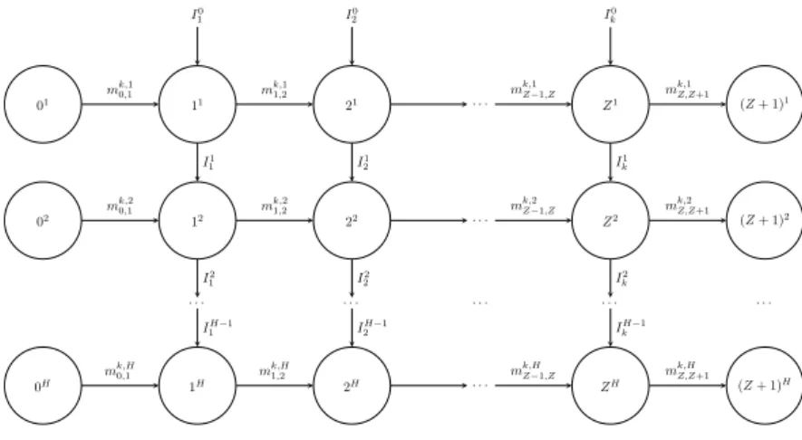
3.2 Network with mass and inventory flow for vehicle k . . . 53

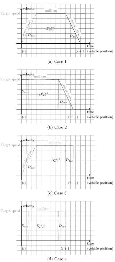
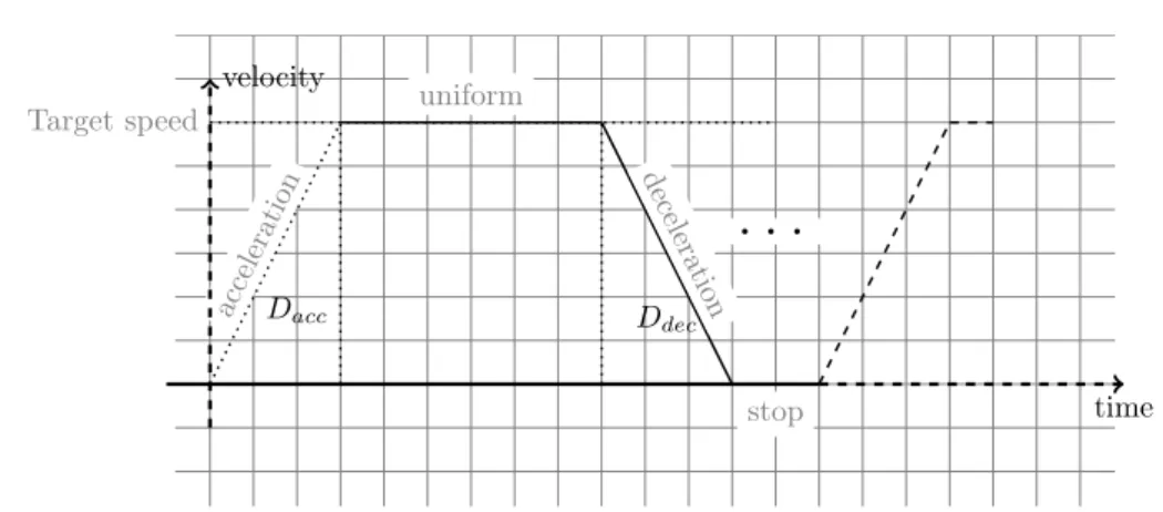
3.3 Vehicle speed profile scenarios . . . 57

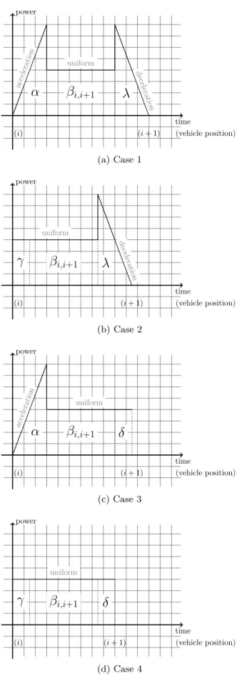
3.4 Vehicle power change scenarios . . . 58

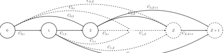
3.5 Simple graph for the supply chain with energy cost Ce i,j on arc (i, j) 59 3.6 Simplified multi-graph for the supply chain with different energy costs on arcs . . . 59

4.1 The speed variation of the vehicle with time . . . 69

4.2 The flows passing through customer i at period t . . . 73

4.3 Number of customers and energy reduction . . . 78

4.4 Distance or inventory cost and energy cost under different configu-rations . . . 79

4.5 Vehicle routes under different objectives . . . 80

4.6 Distance and energy cost under different road types . . . 81

4.7 Inventory and energy cost under different inventory policies . . . 81

5.1 Solution method in three steps . . . 100

5.2 the definition of slack θd,tl,i for driver/trailer pair (d, tl) and customer i101 5.3 Example profits of visit . . . 117

5.4 Example of a time-space graph of a trailer with two customers . . . 118

6.1 Example with 1 depot and 2 customers . . . 132

(13)

(14)

List of Tables

3.1 CPU time in seconds for the determination of Emin. . . 63

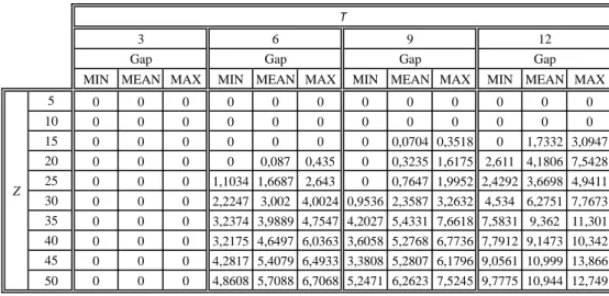
3.2 Gaps to optimality in percentage. . . 63

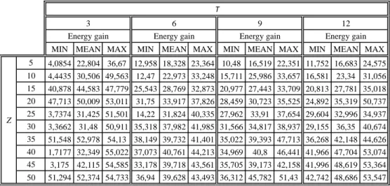
3.3 Energy savings in percentage. . . 64

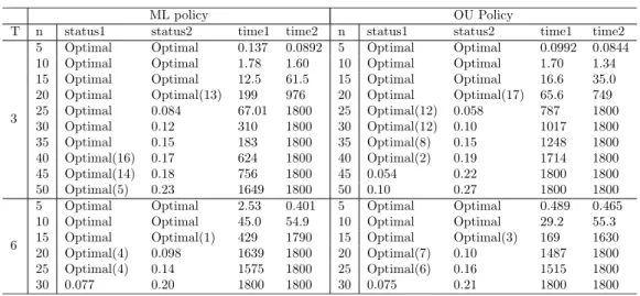
4.1 Solution status and solving time . . . 77

5.1 Notations . . . 96

5.2 Parameters fixed by the greedy heuristics . . . 105

5.3 Variables in the FS-MILFP model . . . 105

5.4 Results for the Final Instances Set B . . . 121

5.5 Characteristics of the Instances Set B and X . . . 122

5.6 The number of feasible solutions obtained by the two greedy heuris-tics on instances H . . . 123

5.7 The average difference of logistic ratio given by the two greedy heuris-tics on instances H . . . 123

5.8 The heuristics alone vs the heuristics with FS-MILFP on instances H 124 5.9 The improvement by the RT-MILFP with column generation com-pared to that by the heuristics with FS-MILFP on instances H . . . 125

5.10 The RT-MILFP with column generation and the heuristics with FS-MILFP on instances C . . . 127

6.1 Routing details of the solutions . . . 135

6.2 Solutions given by CPLEX for models with and without time flow variables . . . 148

6.3 Bounds obtained by the decomposition method with and without time flow variables . . . 149

(15)

(16)

Introduction

With limited natural resources, energy has become a critical factor for the sustain-able development of human beings. Energy consumption has been closely related to the global economic development. Of all the world energy production, 81.2% is attributable to fossil fuels [87].

Nonetheless, the reserves for fossil fuels are quite limited. They could possibly run out by the end of this century with today’s consumption rate. Besides, due to the massive consumption of the fossil energy resources driven largely by eco-nomic and population growth, the high emissions of Greenhouse Gases (GHGs) are extremely likely to have been the dominant cause of the climate change in recent decades [89].

This alarming energy situation requires a reflection on the use of energy and a change in our energy consuming behaviours. According to the World Energy Out-look 2016 of International Energy Agency (IEA), the energy efficiency improvement in various economic sectors could be the motor of change [88].

Industry and transport sectors account for more than 60% of the total final energy consumption worldwide [87]. However, in most of the time, attention is only paid to the economic benefits. The energy efficiency is considered less vital and the potential energy savings are often neglected compared to the economic ones. Therefore, the energy efficiency of the industrial production and transportation systems needs to be taken into consideration. Reports have shown that by adopting renewable energy consumption scenarios with emphasis on sufficiency and efficiency, it is possible to reduce by half the final energy consumption by 2050, while ensuring the same level of energy services [106].

To achieve a future with efficient energy usage, the first step is to study the current systems with energy consideration. This has led to concepts such as Energy Aware Manufacturing (EAM) [110], green logistics, sustainable supply chain man-agement [68], to name just a few. In this thesis, the energy issues of the supplying systems with vehicles are studied explicitly.

In general, the problem studied in this thesis is a problem of combinatorial optimization. It belongs to a family of problems called Vehicle Routing Problems (VRPs). This family of problems is concerned with the distribution of products using a set of vehicles in a transportation network. The VRP has been studied for nearly 60 years and it is still an active area of research with many applications [47, 98]. It involves decisions on which route to take by each vehicle to serve a set of customers under certain restrictions such as the vehicle capacity. The demands of customers are assumed known in advance and are not part of the decisions. The objective is to minimize the total costs of routing. In most of the cases, it is the economic costs such as the distance or the total travel time that are considered.

Since the 1980s, a variant of VRP has emerged under the context of fast evo-lution of information systems, deriving the so-called Inventory Routing Problem

(17)

(IRP). In this variant of routing problems, the decisions on transportation and inventory management are taken simultaneously. It consists of monitoring the in-ventory levels of a set of customers. Deliveries are made whenever it is necessary and cost efficient. It usually expands to a horizon of several days or even longer. A particularity of this problem is that the demands of the customers are now consid-ered as decisions. In addition, decisions made at one period of time influence the decisions to make later. The objective function often includes costs of both inven-tory storage and transportation. The combined decisions in the IRPs can improve the economic efficiency of the inventory management systems. However, the energy issue in the IRP was seldom studied.

Recently, as people are becoming more and more concerned with the energy is-sue, Green Vehicle Routing Problems (GVRPs) emerge as a new variant of VRP. It concerns a family of VRPs with a consideration for energy-efficiency, air-pollution or GHG emissions. In GVRPs, the ecological aspects are integrated into different variants of VRPs by setting new objectives, adding more constraints or new deci-sion variables. It has been shown that the current transportation systems can be improved to be more energy-efficient [25, 64, 72].

Although GVRP is a popular area of study for the integration of energy issues into transportation systems, the study on the energy aspect of the IRP has just started. The problems studied in this thesis are an integration of energy consid-eration into the IRP. It models the energy as a cost that is linearly dependent on the transported mass, which links the inventory control and the product routing. It identifies the most influencing factors to vehicle energy consumption and shows the potential energy improvement in the current inventory routing systems. New features introduced to the IRP by the energy aspect are also highlighted.

According to the theory of complexity, the combinatorial optimization prob-lems can be classified into P—probprob-lems that can be solved in deterministic poly-nomial time, and NP—problems that are solvable in non-deterministic polypoly-nomial time [77]. The category of VRPs is one of the most famous set of NP-hard prob-lems and unless the condition P = NP is proved to be true, it cannot be solved by a polynomial algorithm. To deal with such problems, there are mainly two ways: one is heuristic methods that are fast but do not guarantee the optimality of the solution. The other is exact methods which ensure the quality of solution but are more computationally expensive.

With the ecological considerations, the problem usually gets much more compli-cated. Various approaches have been used to solve the GVRPs. Most of them are adapted from the methods for solving the VRPs. For the IRP, various heuristics exist, as well as a few exact methods. In this thesis, several mathematical models for the solution of the IRP with energy consideration are proposed. These models are helpful for developing advanced solution methods based on mixed integer pro-gramming. Decomposition methods based on column generation are also applied to solve a real-life IRP. Lagrangian relaxation based decomposition is provided for solving a simple version of the real-life IRP with energy consideration.

(18)

Combi-3

natorial Optimization and Constraints (ROC)” of the Laboratoire d’analyse et d’architecture des systèmes of Centre national de la recherche scientifique (LAAS-CNRS) in Toulouse, France. It has been funded by the grant program called “Al-location Prioritaire Thématique” of the University of Toulouse III Paul Sabatier.

The thesis is divided into three parts, each part with two chapters:

Part I is the state of the art. Chapter 1 defines the combinatorial optimization problems in general, presents the VRPs and several variants that has been useful to integrate the energy aspect. It also explains the basic methods for the solution of these problems. Chapter 2 presents the IRP and the GVRP. Different types of IRPs are reviewed with regard to different application backgrounds. Common solution methods for the IRPs are presented as well as some well-known benchmarks. The GVRPs is then introduced with a discussion on energy modelling methods and energy influencing factors. Solution methods for the GVRPs are also presented with some of the benchmarks seen in the literature.

Part II is dedicated to the integration of the energy consumption into supplying and routing problems. Two problems are studied in details in this part. One is the Energy-Efficient Assembly-line Vehicle Supplying Problem (EEAVSP) and the other is the Inventory Routing Problem with Energy Consideration (IRP-EC). In Chapter 3, the EEAVSP is presented. It is a raw-material feeding problem encountered inside the assembly lines, with one fixed delivery route per period. The energy consumption of a vehicle is estimated according to the vehicle dynamics in relation to the supplying planning and the transported mass, assuming a fixed speed profile. Since the energy consumption is linearly dependent on the transported mass, two mathematical formulations based on the flow of mass are presented. The results show that the energy consumed by the transportation of spare parts in a supply chain is connected with the planning of the feeding activity. It can be highly reduced by making better decisions on the feeding quantity and time. Chapter 4 generalizes the EEAVSP to road networks and defines the IRP-EC. The energy cost is added as an objective for the inventory routing. Energy consumption of a vehicle is estimated in the same vein as for the EEAVSP by adding information on traffic conditions on road networks. The results of the experiments reveal the importance of energy consideration for the combined inventory management and routing systems.

Part III includes a real-life IRP in Chapter 5 and a simplified version with en-ergy consideration in Chapter 6. The real–life IRP is adapted from the ROADEF 2016 Challenge problem [6]. It considers many industrial constraints and deci-sions that are not commonly dealt with in classic IRPs, such as the scheduling of the drivers, the timing of visits and the continuous monitoring of the customer inventory levels, among others. It is solved using a decomposition method based on column generation. In Chapter 6, a simplified version of the real-life IRP is presented with consideration on energy consumption. This version keeps the de-cisions on the timing of visits and inventory monitoring in continuous time, and adds the energy consideration. Since travel duration can influence both the energy consumption of the vehicle on a road segment and also the inventory variation of a

(19)

customer, a multi-graph model is proposed, where each arc is characterised by the cost of energy as well as the travel duration. The solution method for this Multi-Graph Inventory Routing Problem with Energy Consideration (MG-IRP-EC) is a decomposition method based on Lagrangian relaxation. Some preliminary results are given at the end.

(20)

Part I

(21)

(22)

1 Routing Problems and Solution Methods 11

1.1 Combinatorial Optimization . . . 11 1.2 Vehicle Routing Problems . . . 12 1.2.1 Travelling Salesman Problem . . . 13 1.2.2 Capacitated Vehicle Routing Problem . . . 13 1.2.3 Other Variations of Vehicle Routing Problems . . . 14 1.3 Solution Methods . . . 16 1.3.1 Heuristics . . . 16 1.3.2 Tools for Developing Exact Methods . . . 17 1.3.3 Decomposition Methods Based on Mathematical programming 20 1.4 Conclusion . . . 23

2 IRP and GVRP 25

2.1 Inventory Routing Problems . . . 25 2.1.1 Problem Presentation . . . 26 2.1.2 Applications . . . 26 2.1.3 Classification of the Inventory Routing Problems . . . 27 2.1.4 Solution Approaches in the Literature . . . 31 2.1.5 Benchmarks . . . 32 2.2 Green Vehicle Routing Problem . . . 32 2.2.1 Problem Presentation . . . 32 2.2.2 Energy Estimation . . . 34 2.2.3 Key Factors Affecting Energy Consumptions . . . 35 2.2.4 Solution Approaches . . . 36 2.2.5 Benchmarks . . . 36 2.3 Conclusion . . . 36

(23)

(24)

Table of Contents 9

In combinatorial optimization, routing is an important part that intervenes in many applications. During all these years, with various application contexts, the problem has evolved and transformed into different variations.

With the development of the information systems, there is a trend to integrate different parts of a large system to achieve a better performance of the whole sys-tem. The IRP is a beautiful example of this integration. It considers inventory management and routing at the same time for a more efficient utilisation of re-sources.

On the other side, in a world with limited natural resources, energy issues are becoming more and more important. The integration of energy consideration is a new tendency among both practitioners and academic researchers. The GVRP is an emergent area of study that analyses the environmental aspect of the distribution systems.

This part is dedicated to the state of the art. In Chapter 1, we make a brief literature review of the general routing problems and principles of some solution methods that are relative to the works presented in this thesis. In Chapter 2, the IRP and the GVRP are presented in general and the integration of energy consumption into the IRP is introduced.

(25)

(26)

Chapter 1 Routing Problems and Their

Solution Methods

Combinatorial optimization arises in everyday applications such as assignment, transportation, scheduling and so on. The Travelling Salesman Problem (TSP) is one of the most widely studied problem of combinatorial optimization. A natural generalisation of the TSP is the VRP, which concerns the distribution of products from central depots to final users.

This chapter introduces the general notion of the routing problems and their solution methods. We start with a formal definition of combinatorial optimization. Then the TSP is presented, which also serves as an example to show the modelling by graph and as an introduction to the notion of complexity. After that, several types of VRPs where energy issues can be integrated are presented. A brief review of some basic solution techniques concerned in this thesis is provided in the end.

1.1 Combinatorial Optimization

To optimize means to minimize (or maximize) a measure of performance of a system by choosing the value of certain variables under certain restrictions. A mathematical model in operations research is the system of equations and related mathematical expressions that describe the essence of the problem [86]. It usually contains a set of quantifiable decision variables, a set of constraints, and an objective function. The constraints are mathematical equations/inequalities or logical relationships for the restrictions of values that can be taken by each variable. The objective is typically a mathematical expression of the decision variables for the measure of performance. The constants (namely, the coefficients and right-hand sides) in the constraints and the objective function are called the parameters of the model. An instance of an optimization problem is a data set for the parameters. The mathematical model might then say that the problem is to choose the values of the decision variables so as to minimize (or maximize) the objective function, subject to the specified constraints [86].

Mathematically, a general optimization problem of n variables in R can be defined as:

minimize c(x)

(27)

where the set S ⊂ Rn _{is defined by some constraints and x ∈ S is a vector of n}

variables. In particular, if the constraints and the objective are all linear and variables are all continuous, then the problem is called linear and can be solved by Linear Programming (LP).

The set S is called the search space or feasible region of the problem. If S 6= ∅, then the initial problem is feasible and S defines the set of feasible solutions. A solution x∗ _{such that ∀x ∈ S, c(x}∗_{) ≤ c(x) is called a globally optimal solution. For} a subset S1⊂ S, if x1 has the property that ∀x ∈ S1, c(x1) ≤ c(x), then x1 is called a local optimum.

If an optimization problem contains a set of M ≥ 2 objective functions (c1, c2, . . . , cM) it is a multi-objective optimization problem. In the

minimiza-tion case, a soluminimiza-tion x1 is said to be dominated by a solution x2 if and only if ∀i ∈ {1, 2, . . . , M}, c_i(x₁) ≥ c_i(x₂) and ∃j ∈ {1, 2 . . . , M}, c_j(x₁) > c_j(x₂). A solu-tion x ∈ S is called Pareto optimal if it is not dominated by any other x0_{∈ S}_{. And} the set of Pareto optimal solutions defines the Pareto optimal set and its mapping in the objective space is called the Pareto front.

The distinguishing feature of discrete, combinatorial, or integer optimization is that some of the variables are required to belong to a discrete set, typically a subset of integers. These discrete restrictions allow a mathematical representation of phenomena or alternatives where indivisibility is required or where there is not a continuum of alternatives [107].

Generally, let N = {1, . . . , n} be a finite set and c = (c1, ..., cn) be an n–vector.

For F ⊆ N, we define c(F ) = X

j∈F

cj. Given a collection F of subsets of N, the

combinatorial optimization problem is defined as [107]:

CP:

minimize c(F )

F ∈ F

If the problem is linear and if the set N contains both continuous and inte-ger values, then this problem is considered a Mixed Inteinte-ger Linear Programming (MILP) problem.

In the following section, the TSP is introduced followed by the presentation of a category of combinatorial optimization problems—the VRPs, which is the basic problem of this thesis.

1.2 Vehicle Routing Problems

Vehicle Routing Problems (VRPs) is a family of problems encountered notably in transportation. These problems are to find the most efficient way to dispatch either passengers or goods from central origins to certain destinations under certain restrictions. In addition to the application in transportation and logistics, VRPs

(28)

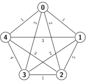
1.2. Vehicle Routing Problems 13 4 0 3 2 1 1 1 3 2 2 2 3 4 ₅ 1

Figure 1.1: Example of TSP with five cities

are also widely applied to the design of electric circuit or computer networks, for instance.

1.2.1 Travelling Salesman Problem

Given a list of cities, a salesman, starting from his home city, is to visit each city on the list exactly once, and return home. Suppose that the salesman knows the distance between each two cities, the Travelling Salesman Problem (TSP) is to find the order of visit to each city to minimize the total travelled distance from all the possible combinations of the orders. The TSP is one of the most studied combinatorial problems. Figure 1.1 shows an example of TSP with five cities. Each city is represented by a node numerated from 0 to 4 and the cost between each pair of cities is marked by the number beside each arc of the graph. This example shows a symmetric TSP since the graph is not directed.

To solve such a problem is not easy. Actually, the TSP as expressed above can be categorized into a type of problems called “NP-hard”. That is to say, all the problems in the class of Non-deterministic Polynomial time (NP) can be reduced to the TSP [82] and unless the condition P = NP is proved to be true, it is not sure to be solved by a polynomial algorithm.

A formal mathematical definition of the TSP can be given using some notations in the graph theory. Let G = (V, A) be a graph (directed or undirected) with V the set of vertices and A the set of arcs. Each vertex represents a city and each arc (i, j) ∈ A represents the way between two cities i and j. The distance Dij

between each pair of cities i, j ∈ V is assumed known. The tour that visits each city in the list once and exactly once is also called a “Hamiltonian cycle” in the graph theory. Then the TSP is to find a tour (Hamiltonian cycle) in G = (V, A) such that the total costs of edges on the tour is the smallest.

1.2.2 Capacitated Vehicle Routing Problem

In general, Vehicle Routing Problems (VRPs) are a family of problems that consid-ers the distribution of goods to a set of customconsid-ers in a given time period by a fleet (a set of vehicles). The vehicles are located in one or more depots and operated by a set of drivers. They move inside an appropriate road network. In particular, the

(29)

solution of a VRP calls for the determination of a set of routes, each performed by a single vehicle that starts and ends at its own depot, such that all the requirements of the customers are fulfilled, that all the operational constraints are satisfied and that the global transportation cost is minimized. [124]

The Capacitated Vehicle Routing Problem (CVRP) is the simplest and most studied member of the family of VRPs. It first appeared in [47] under the name of “truck dispatching problem”. In this problem, there is a set of customers Z, each i ∈ Z having a known non-negative demand Ri to be delivered by a fleet K of

identical vehicles, each with the same capacity B. Each time the vehicle traverses an arc (i, j), there is a cost ci,j that can be either the distance or the travel time

on this arc. In the CVRP, each vehicle performs at most one route. Each route starts and ends from a central depot and visits each customer at most once. Each customer is visited by at most one vehicle route.

The CVRP is a generalisation of the TSP since in each vehicle tour a TSP has to be solved. What distinguish the CVRP and the TSP is the fact that B P

i∈ZRi,

so all the customers cannot be delivered in the same vehicle route. To ensure feasibility, it is assumed that Ri ≤ Bfor all i ∈ Z. The total demands of customers

visited in one route should not be larger than the vehicle capacity. The objective is to find the routes of vehicles that minimize the total costs of arcs belonging to the routes.

The CVRP is at the source of many routing problems. Please refer to the book [125] for the presentation of the problem and its solutions. A more recent book [127] presents the VRP with some new variants and new solution methods. In the remainder of this section, several variants are briefly presented as basic problems of the IRP and GVRP that we are going to present in Chapter 2.

1.2.3 Other Variations of Vehicle Routing Problems

Closely related to real-life applications, the VRP has attracted extensive research attention for over 50 years. Interests for the VRPs have never ceased and efforts are continuously being made to develop more realistic models and more efficient algorithms. Here are some variants of VRP that are mentioned in Chapter 2 to show the wide possibility of the integration of energy consideration into routing problems.

1.2.3.1 Vehicle Routing Problem with Time Windows

The Vehicle Routing Problem with Time Windows (VRPTW) is the extension of the CVRP where the service at each customer must start within an associated time window and the vehicle must remain at the customer location during service [45]. In addition to demand, each customer is associated with a visiting time window defined by an earliest and a latest visiting time, and also a service time smaller than the duration of the time window. Each visit of a customer by a vehicle must be included in the corresponding visiting time window. The VRPTW models can

(30)

1.2. Vehicle Routing Problems 15

better reflect the situation where customers are not open all the time. The presence of time windows can also have an influence on the energy consumption on route. For example, in order to arrive in time to a customer, the vehicle might choose a fast route with more consumption than a slow one with less consumption.

1.2.3.2 Time-Dependent Vehicle Routing Problem

Traditional VRP considers constant travel distances or travel times. This is obvi-ously not true in the real road network where traffic parameters change from the morning to the night. The distinctive characteristics of the Time-dependent Vehi-cle Routing Problem (TD-VRP) is that the travel time between any pair of points depends on the starting time of tour, the starting time of traversing an arc, or the distance between the points. An early review of the TD-VRP can be found in [104]. Due to its distinctive characteristics, TD-VRP is relevant and useful to account for the actual conditions such as urban congestion, where the speed of the vehicle is not constant (as well as the travel time) due to variation in traffic density as in [71]. Since speed and travel time is important for energy, the TD-VRP is often considered a starting point for energy integration.

1.2.3.3 Vehicle Routing Problem with Heterogeneous Fleet

The VRP with heterogeneous fleet can be seen as an example of “rich” VRP which is closer to the reality with multiple depots, multiple trips per vehicle, multiple vehicle types and so on. In the VRP with heterogeneous fleet, the vehicles are not identical. They are often associated with different capacities and different using costs. Together with the VRPTW, the problem could also account for the situation where the vehicle works in different times of a day. In addition, different types of vehicles could introduce different energy costs because of their different weights and engine powers. Please refer to the book chapter [19] for a detailed review of the VRP with heterogeneous fleet.

1.2.3.4 Vehicle Routing Problem with Pickup and Delivery

In the Vehicle Routing Problem with Pickup and Delivery (VRPPD), a heteroge-neous fleet based at multiple terminals must satisfy a set of transportation requests. Each request is defined by a pickup point, a delivery point and a demand to be trans-ported between these two points. There are often time windows to be satisfied at each stop [50]. In addition, the pickup and delivery points are to be visited exactly once in a route of the same vehicle without exceeding the capacity of the vehicle. Precedence constraints are also imposed to make sure that pickup points are visited before delivery points. The vehicles should return to the corresponding terminals at the end of each tour and there are resource restrictions on the number of drivers and vehicle types. The VRPPD can model the problem for the pickup and throw of wastes in urban areas [14, 54].

(31)

1.3 Solution Methods

For solving NP-hard problems in general, two strategies are applied in practice. The first defines the category of solution methods called “heuristics”, which is fast and accepts the possibility of a suboptimal solution, while the second is called the “exact methods”, which focus on the optimality of the solution but can be very time-consuming [100].

In this section, a brief review on these two categories methods is made with emphasis on exact methods. Then, decomposition methods for solving real size instances are particularly introduced to make clear some basic ideas of the solution methods applied in this thesis.

1.3.1 Heuristics

The heuristics are fast solution methods without optimality guarantees. There are many types of heuristics for the solution of combinatorial optimization problems. Simple heuristics are often applied to find an initial feasible solution in a short time for further improvement. The metaheuristics are methods that employ special strategies to explore the neighborhood structures of complex solution spaces.

Taking the VRP as an example, classical heuristic methods include constructive heuristics, two-phase heuristics and improvement methods [99]. The constructive heuristics gradually build a feasible solution while keeping an eye on the cost. The two-phase heuristcs decompose the solution into two parts, one aiming at clustering vertices into feasible routes and the other constructing the routes. The improve-ment methods upgrade a feasible solution by performing a sequence of edge or vertex exchanges within or between vehicle routes. Besides, there exist a wide va-riety of metaheuristics. The most popular and successful ones for the VRP are, among others, Simulated Annealing (SA), Tabu Search (TS), Genetic Algorithms (GA), Greedy Randomized Adaptive Search Procedure (GRASP), Variable Neigh-bourhood Search (VNS) and Adapted Large NeighNeigh-bourhood Search (ALNS). For a literature review on the heuristics and metaheuristics for the CVRP, please refer to the book chapters in [125].

Recently, there is a new category called “hybrid metaheuristics” that integrate various solution methods and take advantage of each of the integrated methods. The hybrid methods may exclusively combine metaheuristic concepts, or also involve algorithmic ideas and modules from mathematical programming, deriving the so-called “matheuristics”. Efficient solution methods can also be obtained by the joint effort of heuristics with constraint programming, tree-search procedures, to mention a few [131]. For a survey of such hybrid metaheuristics, please refer to [115]. More recently, a new category of heuristics called “hyper-heuristics” is emerging for the solution of industrial problems. Although not annonced officially, the ALNS can be seen as a simple version of hyper-heuristics. The hyper-heuristics operate on a search space of heuristics (or heuristic components) rather than directly on the search space of solutions [32], which tries to automatically design or select the

(32)

1.3. Solution Methods 17

adapting heuristic methods according to the structure of the problem.

1.3.2 Tools for Developing Exact Methods

Contrary to the heuristics that are content with finding rapidly a good solution even if it is suboptimal, the exact methods insist on the optimality of the solution, even though a lot of computation time may be spent. Classic exact methods for the VRP include direct tree search methods and Dynamic Programming (DP). They are usually derived from some special mathematical programming formulations.

In the following, we first introduce some of the mathematical formulations of CVRP , which have been used to derive exact methods in the literature and have also inspired some of the formulations in this thesis. Then, the principles of the Branch-and-Bound (B&B) are presented, which served as the general solution scheme for many exact solution methods. After that, the dynamic programming method are sketched. For a recent review of exact methods for CVRP please refer to [20, 119, 126].

1.3.2.1 Mathematical Programming

To apply the mathematical programming to an optimization problem in general, the first step is to formulate the problem using a mathematical model. Solution approaches vary a lot from one formulation to another. For the CVRP, there exist different types of formulations. In the following, we present three most common mathematical formulations for the CVRP ordered by the number of index of the principal variables.

Remember that the problem is modelled on a graph G = (V, A). Node 0 de-notes the depot. Other nodes denote customer locations. Let Z denote the set of customers, each with demand Ri. Let K denote the set of vehicles, each with the

capacity B. The total number of vehicles is denoted by K.

One index formulation In this formulation, the CVRP is considered as a Set

Partitioning Problem. Let Ω be the set of feasible routes. A feasible route is defined as a route starting and ending at the depot that make a hamiltonian tour among the set of customers to satisfy their demands. Binary parameter ai,r equal to 1 if

the customer i ∈ Z is in the route r, 0 otherwise. Cost cr for each route r ∈ Ω is

computed as the sum of costs of arcs taken in the route. Binary variables λr equal

to 1 if the route r is selected and 0 otherwise. The CVRP is then formulated as

minimize X r∈Ω crλr subject to X r∈Ω ai,rλr= 1 ∀i ∈ Z X r∈Ω λr= K

(33)

λr∈ {0, 1} ∀r ∈Ω

This formulation was first proposed in [21]. It is a binary integer formulation with potentially exponential number of variables. It is very general and can take into account various constraints on a route since route feasibility is implicitly considered in the definition of the set Ω. It can also serve as basic formulation for the column generation scheme detailed in section 1.3.3.1.

Two index formulation This type of formulation is also known as vehicle flow

formulation or assignment based formulation. It contains an explicit arc-based binary variable xi,j, which equals 1 if arc (i, j) is used in a solution, 0 otherwise.

xi,jcan be seen as a flow variable for the number of vehicles circulate on an arc (0 or

1). Let ci,j the cost of arc (i, j), and for each set S ⊂ Z, r(S) the minimum number

of vehicles needed to serve the customers in S. The CVRP can be formulated as:

minimize X (i,j)∈A ci,jxi,j subject to X i∈Z x0,i = K X i∈Z xi,0 = K X j:(i,j)∈A xi,j = 1 ∀i ∈ Z X j:(i,j)∈A xj,i = 1 ∀i ∈ Z X i /∈S X j∈S xi,j ≥ r(S) ∀S ⊂ Z (SEC1) xi,j ∈ {0, 1} ∀(i, j) ∈ A

The constraints (SEC1) is the set of subtour elimination constraints (SEC). It says that for all subset S of Z, there is at least r(S) vehicles entering or leaving the nodes in S. Since these constraints are for all the subsets of Z, which are expo-nential in number, the formulation is not compact. In practice, there are various ways to eliminate the subtours. One way is to add auxiliary variables to generate compact formulation. Another way is the cutting plane method and the algorithm of Branch-and-Cut (B&C). A wide variety of B&C algorithms are derived from this formulations (see [20] for a review of these algorithms).

Three-index formulation Explicit arc-vehicle-based binary variable z_i,jk for the

(34)

It is equal to 1 if arc (i, j) ∈ A is traversed by vehicle k ∈ K, and 0 otherwise.

minimize X (i,j)∈A ci,jzi,jk subject to X i∈Z z_0,ik = 1 ∀k ∈ K X j∈Z z_j,ik −X j∈Z z_i,jk = 0 ∀i ∈ Z, ∀k ∈ K X j:(i,j)∈A z_i,jk = 1 ∀i ∈ Z X j:(i,j)∈A zk_j,i= 1 ∀i ∈ Z X i∈Z Ri X j:(i,j)∈A z_i,jk ≤ Q ∀k ∈ K (SEC2) z_i,jk ∈ {0, 1} ∀(i, j) ∈ A, ∀k ∈ K

This formulation is particularly useful when modelling heterogeneous vehicle fleet. Some formulations contain an additional set of binary variables yk

i which equal to

1 if vehicle k serves customer i and 0 otherwise.

1.3.2.2 Branch and Bound

The Branch-and-Bound (B&B) is a useful tool for solving large scale NP-hard com-binatorial optimization problems. It is often used as a basic scheme, in which different components can be developed according to the structure of the problem concerned.

Let us take a combinatorial optimization problem (CP) in general defined in Section 1.1. It is a minimizing problem with S denoting the feasible region of the problem, c denoting the objective function, LB(S) and UB(S) the lower and upper bound on the objective in the region S, c∗ _{the best objective encountered for the} best current solution x∗_{. A prototype of the B&B is given by Algorithm 1. In this} algorithm, SL denotes a list of feasible regions to be explored.

The key to success of the B&B is often the quality of bounds used to guide the tree search. In addition, different branching strategies can be tried for the partition of the feasible region to speed up the search. Various search strategies can complement the solution process. Diverse bounds derived from different kinds of relaxations can be applied to the CVRP. For detailed presentation of the B&B algorithm applied to CVRP, please refer to the book chapter [119].

1.3.2.3 Dynamic programming

Dynamic Programming (DP) applies to problems with an optimal substructure and overlapping sub-problems. The basic idea of dynamic programming is to break

(35)

Algorithm 1 Branch and Bound

1: Initialize a set SL with a feasible region R0, with associated bounds −∞, +∞

2: while SL 6= ∅ do

3: Select a feasible region R ∈ SL and SL ← SL\{R}

4: Bound the objective c in the region R: LB(R) ≤ c(x) ≤ UB(R) for all x ∈ R

5: if LB(R) ≥ c∗then

6: Discard R

7: else

8: Branch R by dividing it into k subsets R1, . . . , Rk

9: SL ← SLS{R1, . . . , Rk}

10: if U B(R) < c∗ and the associated solution x(R) is feasible (where c(x(R)) = U(S))

then

11: c∗← U B(R) and x∗← x(R)

12: return c∗ and x∗

down the initial problem into a sequence of overlapping sub-problems, so that the optimal solution of the sub-problems leads to the optimal solution of the initial problem. It is often used as a subroutine in other algorithms. Let us consider a general combinatorial optimization problem with the same notations as given in Section 1.1. The DP can be applied, if the feasible region S can be divided into subsets S0 ⊂ S1 ⊂ . . . ⊂ Sk= S, and the solution of the complete problem can be

decomposed in to sequential solutions of each Sk with f(Si−1, Si) something easy

to solve depending on Si−1and Sifor each i ∈ {1, . . . , k}. A general presentation of

the optimal solution c∗ by dynamic programming can be resumed by Equation 1.1. c∗=

( c(S0)

c(Si) = c(Si−1) + f(Si−1, Si) ∀i ∈ {1, . . . , k} (1.1)

1.3.3 Decomposition Methods Based on Mathematical program-ming

The idea behind the decomposition methods is to decompose the problem into several subproblems that can be easily solved. The solution of one sub-problem can provide information for the solution of other sub-problems or the original problem. By adding feedbacks or adjusting loops between sub-problems and the original one, a good quality solution is obtained in an acceptable time. Both the B&B and DP applies this idea by exploring special structures of the problem. Based on the mathematical programming, there exist other ways of decomposition. In the following, we present two classical decomposition methods that has served in this thesis: the column generation and the Lagrangian relaxation.

(36)

1.3.3.1 Principles of Column Generation

In this section, the one index formulation of CVRP (1.2)—(1.5) is taken as an example. This is what we call the Master Problem (MP).

minimize X r∈Ω crλr (1.2) subject to X r∈Ω ai,rλr = 1 ∀i ∈ Z (αi) (1.3) X r∈Ω λr = K (β) (1.4) λr ∈ {0, 1} ∀r ∈Ω (1.5)

Recall that in this formulation, Ω is the set of feasible routes, which are exponen-tial in number. Thus, this formulation contains exponenexponen-tial number of variables λr, ∀r ∈ Ω and the feasibility of a route r is hidden in the definition of the set Ω.

To solve such a problem, one way is to start by solving the linear relaxation of the master problem by relaxing the integrality constraints (1.5).

The appealing idea of the column generation is to work only with a sufficient meaningful subset of variables, forming the so-called Restricted Master Problem (RMP) [53]. In our example, RMP is defined by (1.2)—(1.4). To do this, an iterative approach is needed. In each iteration, we have to solve the RMP to determine the current objective value and the dual values of each set of constraints (denoted by αi, β on the right of constraints (1.3)—(1.5)). Then, we try to find a

variable λr to enter RMP by solving a pricing problem defined by:

c∗ = min

r∈Ωcr−

X

i∈Z

αiai,r− β (1.6)

with ai,ra binary variable equal to 1 if customer i is in the route r, and 0 otherwise.

For a fixed route r, the value cr−Pi∈Zαiai,r−βis called the reduced cost. Each

iteration of column generation is to find a route (column) with negative reduced cost. If the solution of the pricing problem is negative, then the corresponding variable λr is added to the RMP and the process repeats. Otherwise, there is no

improvement for the linear relaxation of the master problem. The problem is then converted to the initial MP with integer variables. Usually, a branching procedure is used to fix the integer values.

The pricing problem can be seen as a sub-problem of the initial problem. It can be solved by another scheme different from the mathematical programming, such as dynamic programming or heuristics. Thus, it is usually a point of integration when developing hybrid method.

Due to the fact that column generation only works with a sufficient subset of variables, this method is often used to solve large-scale combinatorial optimization problems. However, ensuring a good management of the set of columns is not an easy job. The way to generate columns of good quality within a reasonable size and

(37)

computation time needs special care. Moreover, the solution of the final integer problem after the column generation stays also a big challenge.

The column generation is often implemented as a component of B&B, introduc-ing the so-called Branch-and-Price (B&P). In B&P, the linear relaxation in each node of a branch-and-bound tree are solved by the method of column generation and the term “price” refers exactly to the solution of the pricing sub-probem. It can also be integrated into a method called Branch-and-Price-and-Cut, where addi-tional cuts to strengthen the relaxation are inserted to the master during the column generation phase according to the information given by the generated columns. The book [51] gives more detailed information about the column generation.

1.3.3.2 Principles of Lagrangian Relaxation

The Lagrangian relaxation is a tool for solving large-scale combinatorial optimisa-tion problems. It works by moving hard-to-satisfy constraints into the objective function by associating a penalty.

Consider an integer problem in general:

P:

minimize cx (1.7)

subject to A1x ≥ b1 (complicating constraints) (1.8)

A2x ≥ b2 (easy constraints) (1.9)

x ∈ Zn+ (1.10)

The idea of the Lagrangian relaxation is to relax the complicating con-straints (1.8) with the so-called Lagrangian multipliers (denoted by γ ∈ Rn

+ here). Consequently, the relaxed problem, called the Lagrangian relaxation with respect to A1_{x ≤ b}1 _{becomes much easier to solve. It is defined as:}

L(γ):

minimize cx+ γ(b1− A1_x₎ _(1.11)

A2x ≥ b2 (easy constraints) (1.12)

x ∈ Zn+ (1.13)

It is obvious that the optimal solution of the (L(γ)) with a fixed γ is a lower bound of the original problem.

If we set zD(γ) = max

x∈χ{cx − γ(A

1_{x − b}1_{)} with χ ⊂ Z}n

+ the domain defined by constraints (1.12). The maximization of zD(γ) defines the following problem:

LD:

maximize zD(γ)

(38)

1.4. Conclusion 23

The problem coincides with the Lagrangian dual of (P) with respect to con-straints (1.8). Its optimal solution gives the best lower bound for the original problem. According to the duality theory, this bound is better than the linear relaxation bound except in the case with integrality property. For details of the theoretical demonstrations, please refer to [78].

The Lagrangian relaxation is often integrated in a B&B scheme. In each itera-tion, the easier relaxed problem with a fixed multiplier is solved to provide a lower bound. Then, the Lagrangian multipliers are updated. Additional component can be added to get a feasible solution from the solution of relaxed problem to update the upper bound. The process repeats until a certain stop condition is reached. In the B&B scheme, the lower bound is given by the best lower bound found by the Lagrangian relaxation, the upper bound is updated by feasible solutions found during the iterative process.

To apply such a method, several issues have to be kept in mind [69]. The first is how to choose the constraints that are to be relaxed. The method only works if the relaxed problem is really easy to solve, since the solution of the relaxed problem will be repeated many times in the whole solution process. The second is how to compute good multipliers. A common way is the subgradient method [69]. The third is how to deduce a good solution to the original problem from the solution of the relaxed problem.

The Lagrangian relaxation is often integrated with some heuristic components for the solution of the relaxed problem or to obtain a feasible solution [46]. It can also be used as a sub-routine for the solution of some large scale problems. [26, 37]

1.4 Conclusion

This chapter has defined the general routing problems and some of its variants. Exact solution methods can be developed from mathematical programming formu-lations. General solution methods such as Branch-and-Bound (B&B) and dynamic programming has been presented. Column generation and Lagrangian relaxation are two decomposition methods based on mathematical programming that are often used to solve large scale instances. These two methods are going to be applied later in Chapter 5 and 6 to solve a real IRP and its integration with energy consideration. In the next chapter, the IRP and the GVRP are presented. The IRP is a gen-eralization of the VRP in which the customer demands are not given by customers but also a decision variable. The compromise between the cost of routing and the cost of inventory storage has to be considered in the IRP. The GVRP is an integra-tion of energy efficiency into the VRP, which is an emerging area of study in recent years.

(39)

(40)

Chapter 2 Inventory Routing Problems

and Green Vehicle Routing

Problems

The Inventory Routing Problem (IRP) has been introduced since the 1980s. It in-tegrates both the vehicle routing and inventory management problems. The Green Vehicle Routing Problem (GVRP) has emerged in recent years covering the en-vironmental issue met in the product distribution or public transportation. This chapter reviews these two problems in detail to give the general problem settings, different variants, well-known benchmarks as well as the solution approaches.

2.1 Inventory Routing Problems

The Inventory Routing Problem (IRP) is developed under the Vendor Managed Inventory (VMI) model. In this model, the vendor (or supplier) is usually the man-ufacturer but sometimes can be a reseller or distributor. He or she acts as a central decision maker and monitors the inventory level of each buyer (customer or retailer) physically or via electronic sensors and messaging. The vendor has to make peri-odic resupply decisions regarding delivery quantities and timing. In practice, with respect to the traditional Retailer Managed Inventory (RMI) where the buyers set orders for the suppliers, the VMI can results in reduced costs and improved ser-vices for both suppliers and buyers. For suppliers, smaller buffers of capacity and inventory are possible as the uncertainty of demands is mitigated. The coordina-tion of services to several customers also allows for more efficient distribucoordina-tion and more predictable delivery planning. For the buyers, they devote less resources to inventory monitoring while having the guarantee that stock-out will never happen. In this section, we start with a general presentation of the problem, followed by a classification and applications, and finish with some of the solution approaches. This is only a brief introduction to show the basic problems considered in this thesis. For a detailed explanation of the IRP, please refer to the tutorials [29, 30], which introduce the IRPs with examples, present different models and policies for different classes of the problems and explain the relations with classical routing problems. An early review is proposed in 1998 by [18] with a first classification, but the problem was named “dynamic routing-and-inventory problems (DRAI)” at that time. The review [10] describes the industrial aspects of combined inventory management and routing in maritime and road-based transportation and gives a literature survey

(41)

of the state of the art in 2010. A more recent comprehensive literature review is provided by [43] with a new classification and more accentuation on solution methods.

2.1.1 Problem Presentation

The IRP is an integration of inventory management and vehicle routing and dis-patching. In general, there are a set of suppliers and a set of customers. Each supplier or customer maintains a set of products in their inventory. Customers consume the products gradually. The suppliers monitor the inventory level of cus-tomers and make deliveries to make sure that no one is out of stock. The products are transported using a fleet of vehicles. Each vehicle has a capacity that should not be exceeded. Each unit of product stored in the supplier or customer has an inventory storage cost. Each unit of product transported on road has a transporta-tion cost. The problem is to find the best distributransporta-tion plan that minimizes the combined costs of inventory storage and transportation.

In summary, there are three simultaneous decisions to make: i) when to serve a customer; ii) how much to deliver when serving a customer; iii) how to route the vehicle among the customers to be served [34].

2.1.2 Applications

In industry, combined routing and inventory management problems are mainly found in road-based and maritime supply chains. An important road-based appli-cation is the distribution of industrial gases or petrol oil using trucks, where VMI model is implemented [35, 56, 61, 62, 118, 121, 136]. In fact, the first studies by Bell et al. in the 1980s [26] were to develop an integrated management system for the distribution of industrial gases. The main characteristics of this type of appli-cation are that the inventory monitoring is performed in a very fine granularity of time (often every few hours) during a very long period of time (weeks or years) and that the stock-out is strictly forbidden or costs a lot. The problem could also be integrated with the scheduling of drivers and the assignment of driver to trucks. Furthermore, constraints on the customer side can also complicate the problem, such as customer time windows or consistency of visits. Other road-based applica-tions include, among others, the distribution of spare parts of the car manufacturing industry [31] and the distribution of perishable goods [12, 101, 8, 123].

The maritime inventory routing for Liquefied Natural Gas (LNG), called LNG-IRP is also an important area of applications [9, 79, 120]. It is different from road-based applications due to specialities met in the maritime context. Normally, the planning horizon of the maritime inventory routing is longer with bigger time granularity. There could be more types of vehicles in the maritime applications, too. Please refer to [10] for the comparison of road-based and maritime IRPs and [40] for a literature review of maritime routing and scheduling.

(42)

2.1. Inventory Routing Problems 27

2.1.3 Classification of the Inventory Routing Problems

Due to the different possibilities of problem settings in practice, a wide variety of IRPs exist in the literature. The following classification is based on that given in [43] with some remarks on recently appeared features .

2.1.3.1 General Settings

Different supply chain structures and lengths of planning horizon generate different versions of IRPs

Types of supply chains According to the applications, different structures of

supply chains are studied. Here we only list the types and some of the related papers. For detailed explanation of different types of supply chains and their impacts please refer to [10].

• one-to-one: there is only one central depot and one single customer. This case is studied in an early paper [57] to show the compromise between the transportation costs and the inventory costs.

• one-to-many: there is one central depot (the supplier) and a set of customers. The transporter makes a tour among the set of customers to deliver products. This is the most commonly studied version of the problem [15, 26, 42]. • many-to-many: there are a set of pick-up points (suppliers) and a set of

deliv-ery points (customers), resulting in a pick-up and delivdeliv-ery routing problem, which is often the case in maritime applications [9, 39, 79, 118].

Planning horizon The length of the time horizon can also change the nature of

the problem. Even though the default setting is the inventory monitoring on a long time horizon, mainly two categories of time horizon are studied in the literature: infinite and finite.

• The problem with infinite horizon is to find the replenishment strategy with minimum costs in the long term. In this category of IRPs, the customer demands are usually given by a rate (fixed or variable) in each time unit. A common type of IRP in this category is the Cyclic Inventory Routing Problem (CIRP), in which the decision on replenishment and routing is defined by cycles that repeat infinitely [4, 12].

• With a finite horizon, the long-term problem is reduced to a short period of time and the adequate costs are chosen to reflect long-run inventory costs [57]. The time horizon can be divided into periods and a routing strategy is to be find for each period [16, 17].

(43)

2.1.3.2 Inventory Decisions and Policies

Based on inventory decisions and inventory policies, the problem can be divided into different categories.

Supplier production It can be fixed, variable or to be determined. Most of the

papers on IRP do not deal with the production side. In general, the supplier is sup-posed to have a fixed production rate higher (or not) than the total demand rate of all the customers [16, 117]. In the LNG-IRP, the production rates of suppliers could be variable over time [116]. The integration of decisions on production, inventory and distribution is studied in [22]. If the production decisions are integrated, the problem becomes a Production Routing Problem [3].

Supplier capacity The supplier capacity can be unlimited or limited. In most

of the literature of IRPs, it is assumed infinite but a cost related to the inventory storage at the supplier is taken into account.

Inventory decisions Concerning the case where inventory is not enough to cover

the demands of customers, mainly two options are applied in practice: one is to make sure that there is always enough inventory in the customers; the other is to allow the shortage of inventory but to pay for it with a huge cost. They correspond to the following two strategies:

• no stock-out or non-negative: a stock-out happens when the customer or re-tailer does not have enough inventory in stock. In most IRPs, stock-outs are strictly forbidden. That is to say, the vendor (supplier) should make sure that the inventory level of each customer is never negative or below a safety level defined by the customer.

• lost sales or back orders: lost sales occur when the customer’s inventory is not refilled in time. Customers that are not able to be refilled in time can also be back logged and treated later. Lost sales or backlogging can be allowed but with a penalty on the total cost [1, 109].

Inventory policy Among the various inventory policies applied in practice, two

of them are often mentioned in the IRP literature: Maximum Level (ML) and Order-up-to Level (OU). Under the ML policy, the inventory level of each customer is flexible but bounded by his capacity. Under the OU policy, the inventory of each customer is automatically refilled to his capacity each time he is visited. The inventory policy can have an influence on the combined cost of transportation and inventory. Most early papers on IRP deal with ML policy. Recent papers usually test both policies to show the possible influence of inventory policy to the decisions of inventory routing. In papers regarding supply chain management, the inventory policy could also be tackled as a decision for optimizing the configuration of supply chains [60, 81], which aids to decide the size of the stock, the control strategies or