Can It Happen Again?
Sustainable policies to mitigate and prevent financial crises
Macerata Italy, Oct.1-2, 20
10
The Myth of Demonetarization of Gold
Jean-Guy Loranger
Université de Montréal
Jean.guy.loranger@umontreal.ca
Abstract
The aim of this paper is to discuss the crisis of the international financial system and the necessity of reforming it by new anchor or benchmark for the international currency, a money-commodity. The need for understanding the definition of a numéraire is a first necessity. Although most economists reject any connection between money and a particular commodity (gold) – because of the existence of legal tender money in every country – it will be shown that it is equivalent to reduce the real space to an abstract number (usually assumed 1) in order to postulate that money is neutral. This is sheer nonsense. It will also be shown that the concept of fiat money or state money does not preclude the existence of commodity money. This paper is divided in four sections. The first section analyses the definition and meaning of a numéraire for the international currency and the justification for a variable standard of value. In the second section, the market value of the US dollar is analysed by looking at new forms of value -the derivative products- the dollar as a safe haven, and the role of SDRs in reforming the international monetary system. In the third and fourth sections, empirical evidence concerning the most recent period of the financial crisis is presented and an econometric model is specified to fit those data. After estimating many different specifications of the model –linear stepwise regression, simultaneous regression with GMM estimator, error correction model- the main econometric result is that there is a one to one correspondence between the price of gold and the value of the US dollar. Indeed, the variance of the price of gold is mainly explained by the Euro exchange rate defined with respect to the US dollar, the inflation rate and negatively influenced by the Dow Jones index and the interest rate.
Introduction
Since the publication in 1981 of the late professor Kindleberger’s International Money, the word numéraire has almost disappeared from economic textbooks. The debate in the 70s was very rich about the international currency, gold and foreign exchange rates. Professor Kindleberger’s remarkable essay on “The Price of Gold and the N-1 Problem” was originally published in the French economic review Économie Appliquée in 1970. Nowadays, most economists reject any connection between money and a particular commodity (gold) and postulate state money. They ignore the need of the international
currency to be linked to the real world by a benchmark as a standard of values or prices
- which is not the same as a unit of account. Following Ricardo’s thinking, they consider money as a mean of circulation and forget or minimize the store of value function. The whole idea of a hoard fund or the existence of a store of value - that can be used for the payment commitments inherited from the past - is completely ignored in a Walrasian general equilibrium for money as it is also incompatible with an equilibrium circuit of money so frequently postulated by some post-Keynesians1.
Through the exchange rate system, each domestic currency is linked to this international currency, and, consequently, is linked to such a benchmark elected as a general
equivalent.2 The main point is how do we define that benchmark and, if necessary, can it
be changed or reinterpreted? Two recent publications invite us to rethink the problem in terms of money-commodity: P. Patnaik (2009), The Value of Money, and D. Bryan & M. Rafferty (2006), Capitalism with Derivatives. Patnaik’s conclusion is that oil is the money benchmark while Bryan and Rafferty’s conclusion is that derivatives are the new
“commodity” (risk as a meta-commodity) serving as a benchmark for money.
The first aim of this paper is to discuss the crisis of the international financial system and the necessity of reforming it by new anchor or benchmark for the international currency. The need for understanding the definition of a numéraire is a first necessity. We will demonstrate the exact correspondence between Walras’ and Marx’s numéraire which is defined as a quantum of a certain commodity assumed to be gold in Marx’s form IV. Although most economists reject any connection between money and a particular
1 The question of disequilibrium in the circuit of capital has already been looked at in Loranger (1982,
1986, 1991).
commodity (gold) – because of the existence of legal tender money in every country – it will be shown that it is equivalent to reduce the real space to an abstract number (usually assumed 1) in order to postulate that money is neutral. This is sheer nonsense because
the equivalence between money and the real world is cut off
.
In addition, it ignores thefact that state money must be connected to the world of finance. A second interest of this paper is to give some theoretical foundation to the recent Chinese position in favour of replacing the US dollar as an international currency by SDRs based on a basket of other currencies. This may be a necessary but not a sufficient condition. The sufficient
condition is to have a market value for SDRs where the price of gold or any other commodity chosen as general equivalent is expressed in SDR and a larger role of the IMF as lender of last resort that can establish confidence in the world money. Finally, with the help of an econometric model, a third aim is to show that a strong link exists between the price of gold and the US dollar. Therefore, the demonetarisation of gold is a myth as well in theory as in reality.
This paper is divided into four sections. The first section analyses the definition and meaning of a numéraire for the international currency and the justification for a variable standard of value. In the second section, the market value of the US dollar is analysed by looking at new forms of value -the derivative products- the dollar as a safe haven, and the role of SDRs in reforming the international monetary system. In the third section, empirical evidence concerning the most recent period of the financial crisis is presented and an econometric model is specified to fit those data. The lengthy last section contains various econometric results. After estimating many different specifications of the model – linear stepwise regression, simultaneous regression with GMM estimator, error
correction model- the main econometric result is that there is a one to one
correspondence between the price of gold and the value of the US dollar. Indeed, the variance of the price of gold is mainly explained by the Euro exchange rate defined with respect to the US dollar, the inflation rate and negatively influenced by the Dow Jones index and the interest rate.
1.0 Numéraire and variable standard of value
Many if not most economists prefer to avoid the discussion about a numéraire by limiting their conception of money within a national framework, thus avoiding the discussion of the international reserve currency. They assume that the central bank is the highest
authority and imposes a consensus by declaring the domestic currency legal tender money. This legal tender status is extended to private commercial banks because the central bank acts as the lender of last resort. Nobody denies that fact but it is no excuse to remain silent about the exchange rate and the need of an international currency that can make a consensus about the general equivalent accepted at the world level. The mobility of capital at the world level is in contradiction with state money. This is the view often repeated by Bryan and Rafferty (2006, ch.6). Neoclassical economists postulate a general equilibrium for money and commodities where money is neutral and based on an abstract number equals to 1.The postulate of money neutrality assumes that money can affect the general price level but has no effect on the output level. By ignoring the store of value function, the quantity theory denies the influence of financial transactions on the real economy and, on the business cycle in particular.3 The Chartalist post-Keynesian school4, following Knapp (1924) and Kaldor (1964), argues that, even if
central bank money is a debt, there is no obligation to reimburse it because …”The general acceptability of both state and bank money derives from their usefulness in settling tax and other liabilities to the state. This… enables them to circulate widely as means of payment and media of exchange” (Bell, 2001, 161)5. A similar view is also
found in Smithin (2009). When applied to the US economy, this concept is equivalent to assume that the US dollar is the numéraire for the whole world. How can a state be a benchmark accepted universally? How can a superpower be a good unit of
measurement for value? Using Keynes’ basic assumption that the money wage rate is fixed in each period (in the short run), Patnaik (2009, ch. 13) well pointed out that the commodity behind such a hypothesis is the labor force and, although paper or fiat money is the only form of money circulation, money still rests on a commodity basis (labor power). The same can be said for the international currency which is nowadays the US dollar if one accepts Keynes’ assumption. However, if the US power is
challenged because its money liabilities exceed its taxation capacity or is no more accepted as a value reserve by the rest of the world, because the money wage rate and inflation are out of control, there is a need for a new consensus concerning the form of the general equivalent at the world level.
3 Our concept of non neutrality of money is extended to the real world: money is a commodity (numéraire)
and a store of value that cannot be reduced to an abstract number, although a change in its price does not affect the relative prices.
4 The term chartalist derives from a latin word meaning ticket or token (Knapp 1924). 5 Note in passing the absence of any reference to money as a store of value.
Chosen as a general equivalent, a money commodity (gold) is isolated from the world of ordinary commodities, but its market price (not its cost) is the key link to money. This fact does not imply that there is a fixed proportion between the US dollar and the price of gold. As already mentioned in earlier works (Loranger 1982), it is more realist to specify the price of gold as a variable standard of value6.
1.1 Definition of Walras’ numéraire
Refering to Kindleberger’s article of the N-1 problem, let [ x1 , x2 , ---, xn-1 , xn ] be a bundle of goods
[ p1 , p2 , ---, pn-1 , pn ] be their absolute prices
Assume that xn is chosen as the general equivalent good (numéraire)
The (n-1) relative prices are [p1 /pn, p2 /pn, ---, pn-1 /pn]
Assume that pn = 1, a usual assumption in an elementary macroeconomic course.
The relative prices are [p1, p2, ---, pn-1], and they are now expressed in absolute
money prices.
According to the definition of a price, it is a quantity of money per unit of a particular commodity. In dimensional analysis, let assume that M is money and xn is gold G.7
[pn] = [M/xn ] = 1 → [M] = [xn]= [ G ] . Therefore, money M is gold G. For most
economists, this is an unacceptable statement. In order to avoid it, they refuse to discuss the absolute price system and prefer to stick to the relative price system, avoiding
committing themselves to choose a particular commodity. In a Walrasian equilibrium, prices are determined when there is no excess supply and demand for any commodity. Such an equilibrium rules out the possibility that money can function as a store of value. Many economists think that by assuming pn =1, they have defined a purely abstract
numéraire with no real foundation. Then xn should be an abstract number [1], which is a
contradiction with respect to the real space to which it belongs by definition8.
6 It should be noted that Keynes’assumption of a fixed money wage rate in each period is also a variable
standard of value since the fixed value in each period is not necessarily the same for each period. Bryan and Rafferty’s assumption is another example of variable standard of value since the value of derivatives can change continuously in time and space.
7 A good introduction to dimensional analysis is F.J. De Jong (1967). In economics, there are four
fundamental dimensions: M, R, T and 1 for money, real object, time and abstract number without dimension. All other variables have secondary dimensions derived from the fundamental ones.
8 The real space cannot contain an abstract number. Another embarrassing question is how can x n be a
universal equivalent outside the community of economists if it is an abstract number with no particular reference to the real world? It would boil down to assume that a dollar is a dollar, a tautological statement.
1.2 The Marxian formulation
Let xA ↔ yB ↔---↔wD ↔ zC be equivalence relations between commodities Let [ A, B, ---D, C ] be the bundle of commodities
and [ x, y, ---w, z ] be their absolute values
Assume that C is chosen as the general equivalent commodity (numéraire). The relative form of values are [x/z, y/z, --- w/z]. Assume that z = 1.
The relative values become [x, y, ---w] and they are now expressed in absolute
money form values. According to the definition of a money form value, it is a quantity of
money per unit of a particular commodity. In dimensional analysis, let assume that M is money defined in a value space and C is in the space of real world. Hence, z = [M/C] = 1 → [M] = [C]. C belongs to the space of physical dimension -for instance a quantum of gold. Therefore, there is no difference between Walras’ and Marx’s numéraire. The numéraire cannot be an abstract number equal to unity: money is linked to the real world and, hence, money matters!
1.3 Definition of a variable standard of value
Let us first define a variable standard of value for G which is elected the general (universal) equivalent for all the other commodities. The word elected means chosen and accepted universally by people around the world9. This may not be the case any
longer. One could speak instead of Marx’s form II – total or expanded form of value – where each commodity is taken as a specific equivalent for other commodities –it could be gold, petroleum, etc- Speculation on certain basic commodities such as oil, potash, aluminum, copper, silver and gold cannot be understood otherwise. Speculators are seeking to protect the value of their wealth by exchanging money for these commodities quoted in US dollar. This is a clear indication that the US dollar maintains a link with the real world of commodities. Money is not neutral or abstract for speculators! If one compares for instance the price of oil and the price of gold between 1979 and 2010, the price of oil is around $75 a barrel (only $35 more than 30 years ago) while the price of gold is around $1200 an ounce, an increase of 26 times its official price ($46) and 3.4
9 Bryan and Rafferty (2006) in a note on page 150 outline that Menger (1892) saw money as a commodity
selected by the market, not nominated by the state. “It is the marketable characteristics of the commodity money …that sets it apart from other possible money: a process of natural selection by market processes. Menger contended that it was these sorts of qualities, not state decree, that saw precious metals be nominated as money.”
times its market price ($355) over that period.10 The price of gold is surely a more
acceptable standard of value, reflecting the successive devaluations of the international currency. For instance, there has been a sharp devaluation of the US$ from1971 to 1979: the price of gold shut up from $35 to $355 during that turbulent period of adjustment (a tenfold increase) and has reflected a devaluation which is close to the inflation rate since 1980. Indeed, the consumer price index in the USA based 100 in 1983 is estimated around 214 in 2008. Knowing that its value was 79 at the beginning of 1980, its value has increased by 2.7 times between 1979 and 2008. With the priced of gold at above $1200 in 2010, its increase is now 3.4 times its market value of 1979. This fact is in accordance with what many observers noticed about gold: in the long run, gold is a conservative investment because its price, after adjustment for inflation, gives a low yield and constitutes a rather stable store of value. Moreover, the quantity of world gold reserve, which was around 1150 millions ounces in 1971, felt to 950 millions in 1979 and remained at that level up to 1988. Although “demonetarisation” of gold was proclaimed, central banks continued to keep a large reserve of gold until 1988 (36%). This level has dropped to 10% over the last twenty years. 11 When calculated in tons,
the decrease is around 150 tons per year during the last 20 years. However, this is less than the recent purchase of 200 tons of gold by the Indian central bank. The demand increase of gold by the private sector for speculative purpose was near 500 tons
between 2007 and 2008. This far exceeds the annual decrease in world gold reserves12.
Therefore, gold remains a safe haven and its price remains important and deserves some explanation.
Assume z(t) is the variable price of gold which is equal to a number ≠ 1. We now add a third fundamental dimension [T] for time or [1/T] per period of time. z(t) = a(t) = [M(t)/G] or [M/T] = [a/T] [G]. What does this mean? Simply that a certain quantity of money per period [M/T] is equal to a certain quantity [a/T] of G for the same period. It is easy to see that, if the price of G is constant over time – for example in a discrete time period - the
10 Statistics from the IMF international reserves gives an estimate of $233 at the end of 1979 and $476 for
1980.Because of the wild fluctuations between the two periods, we take the average figure $355. 8 That proportion was 30% in 1971, 38% in 1978, 36% in 1988, 17% in 1998 and 10% in 2008 (IMF 2008).
12 The most spectacular increase is in the form of ETF: 221 t. in 2008 and 617t. in 2009, (Source: GFMS
dimension T cancels itself on both sides of the equality and we have M = aG, that is M is a certain (fixed) proportion of G during that discrete time period13.
What is the particular nature of G? Marx pointed out clearly (Book1,1967) that G has two use values : one as an ordinary commodity with its price related to its cost measured in term of labor power (congealed and living labor); the second as an extraordinary
commodity used as a general equivalent and its price not related to its cost price. One
can call it the speculative or market price as a reserve of value. It is this price which links
the foundation of money with the real world.14 As outlined by D. Parkinson (G&M
08/22/2009): “….while manufacturers of gold-related products had little use for gold, investors have been gobbling it up. Total demand for investment purposes [in Q2 09] rose 157% from a year earlier…In the first six months of 2009, investment accounted for 45% of total demand; historically, it has been hovering around 10 to 15%.” Updating these data for [Q2 10], the increase is 118% with respect to [Q2 09]. In the first 6 months of 2010, investment accounted for 40% of total demand, (World Gold Report 2010).
2.0 The market value of the US dollar
2.1 The form of the universal currency
In ancient times, each empire had the power to create its own money, allow it to circulate in other countries and support it by conquering the wealth of other nations. Nowadays, the situation is not so different, but the form of value is much more sophisticated with the
financial innovations around the U.S. dollar. In the 80s when I wrote my first essays on
that topic, the international financial markets were not as sophisticated as they are today. We witnessed the development of the euro dollar phenomenon which allowed private banks or other investors to have access outside their domestic financial markets and borrow dollars on the world market. This was particularly useful for countries that had enough credit worthiness and were able to escape the control of the IMF and the World Bank for their development. However, this was insufficient since many developing countries were forced to accept structural adjustment plans with strict conditionality. Continuous deregulation starting in the early 80s with the Reagan administration, led to
13 This is analogous to the Keynesian fixed money wage for a time period.
14 Note in passing that if oil were chosen as the standard of value, its market price is around its cost price
and perhaps below for a number of producers in Canada. Therefore, oil would not have a dual price to reflect its role as a general equivalent. Some economists argue that the quality of a money commodity is the stability of its price. This is certainly not the case of oil the value of which has fluctuated from $140 to $40 a barrel in 2008 and now at $75 in 2010. This fact contradicts Patnik’s choice of oil as the commodity standard at the world level: oil can be a temporary refuge for value but it is not a stable value as he argued.
uninhibited development of financial markets, the emergence of many kinds of derivative products and the securisation of debts (slicing and repackaging debts). The risk factor became a new commodity that could be exchanged on a market like any other financial products. Therefore, ABS, ABCP, CDO, CDS15 etc… became the new craze developed
by Wall Street bankers and their imitators across Europe and in other countries that had enough financial strength to issue and sell them. Since many of these products were difficult to price according to their risk factor, the market for them brutally collapsed and created the biggest financial meltdown at the world level.16
2.2 Expansion of derivatives
The notional value of a derivative contract corresponds to the value of the underlying security (shares, bonds, etc.). Since the underlying security is related to a physical capital asset, the notional value of a derivative is simply another measure derived from that asset which transcends time and space. Therefore, the market value of the derivative contract is the amount of money required to buy the derivative instead of buying the security. This has an important advantage for banks, other financial institutions (hedge funds), firms and individuals. It gives them a leverage to buy large amounts of notional capital with a small quantity of liquidities or by borrowing instead of reducing their liquidity17. Securities can be unbundled, repackaged and sold as another
security where the risk is divided and spread over many other investors who buy ABS, ABCP, CDO, CDS. Bryan and Rafferty (2006) see these financial instruments as a new way to value the firm assets in time and space.
“The central, universal characteristic of derivatives is their capacity to ‘dismantle’ or ‘unbundle’ any asset into constituent attributes and trade those attributes without trading the asset itself” (B&R p.52).
“The commensuration properties of financial derivatives mean that the logic of capital is driven to the center of corporate policy making. Assets that do not meet profit-making benchmarks must be depreciated, restructured and/or sold. The decision not to do so is
15 These acronyms are for Asset Back Securities, Asset Back Commercial Papers, Collateralized Debt
Obligations, Credit Default Swaps.
16 The market collapse for these products was not supposed to happen because all traders were using
financial econometric models based on the assumption of risk randomness. Their model could not
incorporate the systemic risk derived from the mimetic behaviour of investors and concentrated the risk on certain financial institutions. They totally ignored Minsky (1982) hypothesis of financial fragility where risky behaviour (Ponzi finance) increases with the length of the business cycle. See in particular Barbera (2009).
17 Because derivatives are contingent values, they are not reported in the balance sheet of firms. But the
now more readily exposed to market scrutiny, as investment bankers use derivatives and derivatives’ prices to unbundle the performance of the different assets and liabilities of firms” (B.&R p.66).
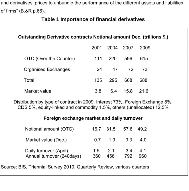
Table 1 Importance of financial derivatives
Outstanding Derivative contracts Notional amount Dec. (trillions $,)
2001 2004 2007 2009
OTC (Over the Counter) 111 220 596 615 Organised Exchanges 24 47 72 73 Total 135 295 668 688 Market value 3.8 6.4 15.8 21.6
Distribution by type of contract in 2009: Interest 73%, Foreign Exchange 8%, CDS 5%, equity-linked and commodity 1.5%, others (unallocated) 12.5%
Foreign exchange market and daily turnover
Notional amount (OTC) 16.7 31.5 57.6 49.2 Market value (Dec.) 0.7 1.9 3.3 4.0
Daily turnover (April) 1.5 2.1 3.4 4.1 Annual turnover (240days) 360 456 792 960 Source: BIS, Triennial Survey 2010, Quarterly Review, various quarters
There is no unanimous consent about the definition and measurement of derivatives. According to the Bank of International Settlements (BIS), the notional amount of OTC derivatives contracts and the notional amount on organised exchanges totalised 688 trillions of dollars at the end of December 2009.The largest part of these transactions is with interest rate (73%). Financial derivatives (interest rate, Foreign exchange and CDS contracts) account for more than 85% of all the derivative contracts. The growth over the 7 year period (2001-2007) is 410%, which represents an average annual growth of 59%. One can observe however that the financial meltdown 2008-09 has brutally stopped that growth which is only 3% since December 2007. However, the market value of these
derivatives has increased by 37% since 2007. Another interesting characteristic of this phenomenon is that transactions on organised markets are continuously loosing ground and represent since 2007 only 10% of the total value of derivative contracts. Even if the foreign exchange contracts represent only 8% of the total transactions, the interest of studying this subsector is in terms of turnover if one wants to impose a tax on this particular type of transaction. One observes a rapid growth of the notional foreign exchange contracts between 2001 and 2007, but this growth stopped and even turned negative (-15%) between 2007 and 2009. As already noted above, its market value has continued to expand (21%) during the same period. The turnover growth over the whole period (173%) is maintained for the last three years (20%). The financial meltdown in 2008-09 had the effect of reducing the stock of outstanding foreign exchange contracts but the turnover increased. The yearly turnover of foreign exchange derivatives is now hovering to 1000 trillions. A Tobin tax of one tenth of one percent would give revenue of one trillion dollars. This is not even the size of the US deficit. The scale of these
transactions may appear to be exaggerated because hedging in financial derivatives (offsetting an existing position) is quite frequent. “Unwinding positions (by means of an opposite trade) in exchange-traded markets tends to result in a growth in turnover, while in OTC markets it tends to add to the notional principal amounts” (B&R p. 57). Anyhow, since the world GDP is estimated around 60T in 2009,18 it is about ten times less than
the notional figure of OTC derivative contracts. A natural question comes to our mind: what is the cause of this amazing development and is it possible to reduce (if not
eliminate) these new financial products - which create and reflect the volatility of financial markets - by a more severe regulation?
According to Bryan and Rafferty, It is not possible neither desirable to eliminate these financial derivatives because they are the new vehicles for storing the value of money.
They consider that derivatives are the new standard of value and form of holding wealth which changes in time and space.
“…valuation across space, time, and between different asset forms is the stuff of derivatives. Derivative traders….operate in a world of perceived equivalence but, and this is critical, it is not a fixed equivalence – for if equivalence were fixed, there would be no need for derivatives” (p. 36).
“[Derivatives] are crucial to the link between money, prices and fundamental value not because they actually determine fundamental values (for there are no truths here) but
because they are the way in which the market judges or perceives fundamental value. They turn the contestability of fundamental value into a tradable commodity. In so doing, they provide a market benchmark for an unknowable value (p.37).”
“[Derivatives] are commodities that manage risk. And because risk exposure is so changeable, the market for these risk management commodities has acquired a high level of liquidity (volume and mobility) with many of the characteristics of money…. Derivatives constitute new private global money (page 38)”.
If derivatives were a benchmark for money, they would constitute universal money like gold. But this is assumption does not stand in the real world. Outside financial
institutions and firms, derivatives are useless as means of exchange and means of payment for ordinary people. It would be more accurate to describe derivatives as a new form of money such as coins, bills, credit cards and credit money that are preferred as a means of exchange and means of payment in particular situations. In fact, Bryan and Rafferty affirm that there is no difference between derivatives and money, but derivatives are a benchmark for unknowable fundamental values. A standard of value for money cannot be an unknowable value because money needs to be defined with respect to a commodity if one wants to maintain a clear distinction between the two fundamental dimensions in economics: money space and real space or real world. In Marxian
analysis, abstract labor values are unknowable values and money is the raison d’être for revealing these values through the market place. Therefore, the definition of the
standard of value or benchmark for money is an unresolved problem.
It would be foolish to eliminate these financial instruments without a major overhaul of the international financial system, because the origin of that new way of trading uncertainty and risks emerged with the regime of fluctuating exchange rates and deregulation in all directions of banking and financial institutions at the world level. According to Bryan and Rafferty, the underlying factors of derivative growth can be summarized as following (p.50):
the end of the Bretton Woods Agreement and the collapse of many national and international commodity price stabilisation schemes;
the increase importance of finance (especially international finance) in investment takeovers, typified by the growth of Eurofinance markets;
the internationalisation of trade and investment, especially with the rise of the multinational firms.
In my opinion, the most important cause is the end of the fixed definition of the US dollar with gold proclaimed in 1971. The Chicago Mercantile Exchange introduced the first derivative on currency in 1972. The Chicago Board of Trade introduced the first
derivative on interest rate in 1975 and the Chicago Board Option Exchange (CBOE) was created in 1973 as a market for options that were previously exchanged as OTC (B&R. p. 94). All these new financial institutions were created to counteract the volatility on exchange rates and other financial instruments (shares, bonds…) after the collapse of the Bretton Woods Agreement.
2.3 The strength of the U.S. dollar and the gold rush
Since the variable exchange rate regime is the consequence of the abandonment of any
official link between the US dollar and gold, what is then the value benchmark of the
dollar as a currency reserve? A bad answer is to state that the value of a dollar is defined by a basket of strong currencies such as euro, yen, Swiss franc, sterling pound, etc …That boils down to say a tautology: a dollar is a dollar! Unfortunately, this is the standard teaching in most macroeconomic
courses.
No wonder then that certain students are quickly disgusted of economics as a science. Economists are unable to justify a fundamental dimension in economics: money - which is at the basis of the definition and measurement of value expressed by market prices - has lost its function of a standard of value and, hence, its function of store of value because its unit ofmeasurement is undefined. As already mentioned previously, this opinion has been challenged by Patnaik (2009) and Bryan and Rafferty (2006). Since the latters’ opinion has been well presented in the previous section, our observations will be limited to Patnaik’s viewpoint.
“A monetary world necessarily requires, according to a propertyist view, the fixity of the value of what is used as money vis-à-vis some commodity, be it gold or silver or labor power… Fiat money is as much commodity money as money fixed against gold; it is just that the commodities in the two cases are different. The world has never succeeded in getting out of commodity money” (Patnaik, pp.163-64). The propertyist view assumes that money is determined outside supply and demand, a view contrary to the monetarist approach and to the post-Keynesian concept of state money.
“State backing can at best confer juridical acceptability, but for it to actually function in the economy in a meaningful manner something more is needed and this something is
the fact that it has a commodity backing, of the commodity labor power, through the fixity of the money wage rate in any single period” (p.164).
However at the world level, the fixed money wage rate in the dominant economy does not apply even if Patnaik admits that …”the possibility of a threat to the value of the dollar through an autonomous increase in the dollar price of labor power in the leading country is remote” (p. 207).
In Patnaik’s view, the stability of the US dollar is nowadays based on the oil price. “It follows that the present currency arrangement hinges crucially on the stability of the price of the dollar in terms of oil, in the sense at least of the absence of persistent declines in it, which is why it can be called the oil-dollar standard. No matter what the de jure situation, the world has not moved away from commodity money” (p.208).
Patnaik finished writing his book in June 2008, just before the start of the financial meltdown that had a tremendous impact on the oil price fluctuating wildly from $140 to a low of $40 and now around $75. Patnaik’s hypothesis about oil-dollar standard is not supported by the recent economic situation. It will be seen in the next section that the price of gold has been much more stable through the crisis and that is the reason why gold is preferred by wealth holders in the present crisis.
Before a new world order emerges, what is happening to the US dollar now?
Paradoxically, despite the near two trillion dollar deficit in 2009 and additional trillions pumped into the monetary system by the FED, the strength of the US dollar has reached a maximum between August 08 and March 09. All currencies have been substantially devalued. For instance, the Canadian dollar lost around 25% between Aug. 1st 08 and
mid-March 09. Euro lost around 20% over that period. Of course, the CDN dollar has completely recovered since.19 The only plausible explanation was a flight to quality by
rentiers and speculators around the world who considered that the U.S. dollar was their
only safe haven. Fearing a global meltdown of the financial order and bankruptcy for
many states, rentiers and speculators wanted to buy U.S. treasury bonds and any other U.S. titles except the toxic assets that created the financial mess. The fear of a serious deflation brought down the value of gold and the price of any other commodities. But it is no more the case in 2010: even if the fear of a deflation is still in the air, the investment demand for gold is boosting its price to new highs as already mentioned in the first section. To paraphrase Patnaik “The current international monetary system,
19 On October 14 2009, the exchange rate was 1.03, the same value as on August 1st 08. On mid-October
notwithstanding its apparent novelty compared to what has prevailed in the past, shares de facto the same general features as the earlier systems”.
This is a unique advantage for an imperialist power: even if its financial system is in a fragile state, the US economy can finance their restructuring debt at a near 0 interest rate with savings coming from the rest of the world. Any other country in such a situation would be declared a failed state. This crisis will last as long as financial instability
continues. It is Happening Again as would have written the late H.P. Minsky (1982). As reported by the World Gold Council (2009), estimated total gold demand for 2008 was 3804 tons, 70% of the world gold demand is for gold as an ordinary commodity (jewellery and industrial/dental use) and 30% for other purposes (investment or reserve value). In 2007 that share was only 19%. An update including the first half of 2009 is pushing that proportion to 46%. In the first quarter of 2009, demand of gold for investment purpose jumped to 60% of total demand. When compared to the same quarter in 2008, the jump represents an increase of 252%. Will this gold rush continue? Let’s quote the opinion of some pundits. According to Parkinson (G&M 03/19/09), “The 2009 recession and banking crisis have set off a rush to invest in gold and other precious metals at unprecedented levels—a move that has tightened the global supply/demand picture and helped push prices to record highs.” Parkinson quotes James DiGeorgia, a dealer in precious metals and editor of the Gold and Energy Adviser newsletter: “People are scared to death that all this debt is going to debase the dollar and other currencies around the world.” Parkinson observes that …”legitimate concerns …have sent investors to gold as a stable safe haven for their money, and a way to diversify their portfolios away from more risky asset classes.”
Parkinson (G&M 09/09/09) quotes again the same guru: “The divergence of opinions is startling. Yesterday, James DIGeorgia …suggested gold could reach $2500 an ounce in the next 18 months and $5000 within five years.”
2.4 Reform of the international monetary system
In March 2009, the governor of the Central Bank of China, Zhou Xiaochuan, launched a call in favour of the need of reforming the International Monetary System. This call received the support of other countries such as India, Russia, France, Brazil, to name only a few of them. The main proposition made by Mr. Zhou is to give an enlarged role to the SDRs as the new reserve currency which would be independent from major currency economies. “As an international currency, the SDR should be anchored to a stable
benchmark and issued according to a clear set of rules”. The main question is how do we define the benchmark? It cannot be simply defined as a basket of other strong
currencies as the SDR is actually defined. Mr. Zhou seems to favour Keynes’ proposition of the Bancor …”based on the value of 30 representative commodities”. Therefore, in Mr. Zhou’s view, the Bancor would not be simply fiat money as proclaimed by Keynesian and post-Keynesian economists. Is it necessary to have 30 commodities instead of one like gold or oil? The economic acceptability of a numéraire depends on the market and not on law or regulation by a superpower or an international institution like the IMF.
Therefore, the market price of gold in SDR is all that is necessary for grounding the international currency to the real world. The importance of a variable price of SDR in gold is to show to the world that a particular commodity is backing the value of money in SDR. This might be seen purely symbolic, but symbols are important in real life. The management of the supply of SDR and its price will depend on a large consensus of the international community to give a larger role to the IMF and, in particular, on the will of the United States to accept that their currency is to be confined to the exclusive role of a national currency. IMF must control the change of the market value of the SDR in a similar way that each country can control the exchange rate of its money. For instance, IMF could favour a controlled devaluation of the SDR in the same way as it can augment the quantity of SDRs like any central bank does when it wants to augment the liquidity in the system. This position is not a return to a gold standard or a gold exchange standard. It is the continuation of the existing state (a variable standard) with a new independent currency. After a transition period, international financial transactions should be done in SDRs instead of US dollars. Then a new international monetary system will bring more stability in the financial markets.
Recall that the suppression of any official link between gold and the international currency reserve of the US dollar caused the phenomenal expansion of derivatives the role of which is to counter balance the risk generated by uncertainty about the store of value function of the international currency. It has also been stated that volatility of financial markets cannot be reduced unless there is a major change in the international monetary system and a new set of regulations. Mr. Zhou seems to share a similar viewpoint.
“The centralized management of part of the global reserve by a trustworthy international institution with a reasonable return to encourage participation will be more effective in
deterring speculation and stabilizing financial markets…With its universal membership, its unique mandate of maintaining monetary and financial stability, and as an
international ‘supervisor’ on the macroeconomic policy of its member countries, the IMF, equipped with its expertise, is endowed with a natural advantage to act as the manager of its member countries reserves (Z. Xiaochuan, p.4, 2009).
.
3.0 Some empirical evidence on the crisis
3.1 The data
The CIRANO Center affiliated to Université de Montréal developed a new tool for analysing the crisis of 2008-09 by collecting a variety of indices from various sources (Chicago Board of Options Exchange, Bloomberg, Standard &Poor, etc…). This tool can combine three indices on the same graph from a pool of 24 indicators. Unfortunately, data are available only for 2008, and the update is not available for 2009.
We first picked the fear index VXO, the Dow Jones index, and the price of gold. We then chose another combination of three variables: the interest rate, the expected inflation rate, and the value of Euro expressed in US dollar. In order to keep the model to a small number of variables, we did not want to include other relevant variables such as net demand for gold, monetary stock and the debt ratio because these latter are most likely strongly correlated with interest rate and inflation.
Euro is most likely correlated with the price of gold since it can be viewed as an alternative to gold for some investors who prefer to speculate on Euro or European assets instead of assets in US dollars or gold. Moreover, Euro being expressed in US dollars is an alternative expression of the value of the US dollar. Therefore, if there is a strong link between Euro and gold price, it will simply illustrate how the US dollar is linked to gold. The series for 2009 have been drawn from various other sources. The expected inflation series is replaced by realized inflation on a monthly basis. An interpolation was done to generate bi-weekly observations. A dummy variable will be specified to take account of the possible discrepancy in the series on inflation between the observations in 2008 and 2009.
Table 1 Evolution of the price of gold with respect to
(source CIRANO) January-October 2009 (other sources) 20
Date Gold VXO DJ Interest Inflation Euro 08/01 914 24 11330 1.63 2.17 1.56 08/15 786 21 11660 1.81 1.95 1.47 09/01 818 22 11540 1.69 1.72 1.45 09/15 832 39 10610 0.23 1.02 1.44 10/01 878 45 10830 0.84 0.95 1.41 10/15 796 70 8980 0.80 0.04 1.35 11/01 728 61 9340 0.44 -0.96 1.27 11/15 738 72 8420 0.14 -1.10 1.27 12/01 779 69 8420 0.06 -0.08 1.27 12/15 875 52 8820 0.05 0.09 1.44 12/31 877 38 9030 0.08 -0.25 1.39 01/15 840 50 8212 0.24 -0.11 1.31 02/01 928 48 8001 0.29 0.02 1.28 02/15 941 45 7850 0.29 0.13 1.28 03/01 948 56 6673 0.27 0.24 1.26 03/15 924 38 7217 0.22 -0.07 1.30 04/01 925 43 7762 0.21 -0.38 1.32 04/15 870 33 8029 0.15 -0.56 1.32 05/01 889 31 8212 0.15 -0.74 1.33 05/15 930 30 8269 0.17 -1.01 1.35 06/01 980 33 8721 0.13 -1.28 1.42 06/15 930 28 8612 0.17 -1.35 1.38 07/01 940 27 8447 0.17 -1.42 1.40 07/15 938 24 8600 0.18 -1.75 1.39 08/01 954 25 9172 0.18 -2.09 1.43 08/15 953 28 9321 0.18 -1.80 1.42
20 Data for 2009 have been drawn from various sources on the web : Kitco.com for gold price, Globe and
Mail MVX, Google finance for the DJ, Federal Reserve for 3 month T-Bill rate and monthly inflation rate, Bank of Canada for the Euro. The series on volatility is an approximation read from the G&M graph when blown to 150%. The series on expected inflation has been replaced and interpolated from the monthly inflation rate in the USA (CPI-all items) between January and October.
09/01 955 27 9496 0.15 -1.50 1.42 09/15 996 22 9683 0.13 -0.75 1.46 10/01 1004 20 9712 0.14 0.20 1.46
There is an obvious inverse correlation between the Dow Jones index and the fear factor VXO. The correlation between the price of gold and the DJ index (or the fear factor) is less obvious: an inverse correlation is observed between August 08 and end of February 09 when the DJ reached its minimum. However, the two series seem to be positively correlated for the last quarter. It coincides with the reduction of fear index. A more rigorous analysis of the data is required.
3.2 An econometric model
The interesting point here is not gold as such, but its variable standard a(t). What are the determinants of a(t)? The short answer is the political, economic, cultural and military power of a dominant nation. In other words, there are countless numbers of
determinants. As usual in economics, the ability of an economist is to select the most important ones and add a random variable for the others.
Therefore, let a(t) =f[X’(t); u(t)]
where X(t) is a column vector of the most significant determinants of the price of gold and u(t) a random variable which accounts for all other (stochastic) influences on the price of gold. With the data chosen, the vector of explanatory variables is
X’(t) = (VXO, DJ, EURO, INTEREST, INFLATION).
Therefore, the linear regression of the price of gold on these five determinants is: z(t) = α+ β’ X(t) + u(t)
where X(t) is a column vector of 5 components, β’ is a line vector of 5 parameters, z(t), u(t) and α are scalars.21 Of course, this simple form can be complicated in many ways
depending upon the assumptions made about u(t) and X(t). If for instance u(t) and X(t) are not independent from each other because of multicollinearity between the
explanatory variables (which is surely the case for some of them), then the model could be transformed into a simultaneous model of two or more equations. It is also quite likely that it is not as much the simultaneous interdependence which matters most, but the lagged response of the price of gold to the various determinants. Some of these
21 A dummy variable(DUM09) is also specified in the regression in order to take into account any
determinants could be expected values instead of actual values. In which case, the model could take the form of
z(t) = α+ β’[H(L) X(t)] + u(t)
where H(L) is an infinite polynomial in the lag operator L. This can always be
approximated by a rational function of two finite polynomials A(L) and B(L) of order m and n respectively. Hence,
z(t) = α+ β’[A(L)/B(L)]X(t) + u(t) or B(L)z(t) = α’+ β’[A(L)X(t)] + v(t).
Therefore, an autoregressive and/or a moving average process can be specified. One can also specify that the vector X(t) is stochastic and an Error Correction Model would be the proper specification (co-integration analysis).
4.0 Regression analysis
4.1 Simple regression
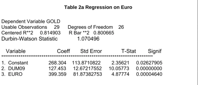
Let us start with the link between the price of gold and Euro which is the key link between gold and the value of the US dollar.
Table 2a Regression on Euro
Dependent Variable GOLD
Usable Observations 29 Degrees of Freedom 26 Centered R**2 0.814903 R Bar **2 0.800665
Durbin-Watson Statistic 1.070496
Variable Coeff Std Error T-Stat Signif
******************************************************************************* 1. Constant 268.304 113.8710822 2.35621 0.02627905 2. DUM09 127.453 12.67217552 10.05773 0.00000000 3. EURO 399.359 81.87382753 4.87774 0.00004640
The price of gold is significantly and positively linked with the value of the Euro defined with respect to the US dollar. Therefore, the price of gold is negatively influenced by the value of the US dollar. The constant and the dummy variables are also highly significant and the explained variance of the dependent variable is at 80%. A low D-W (1.07) indicates the need for an AR(1) correction.
Table 2b Hildreth-Lu regression on Euro
Dependent Variable GOLD
Usable Observations 28 Degrees of Freedom 25 Centered R**2 0.864848 R Bar **2 0.854036 Durbin-Watson Statistic 1.659831
Q(7-1) 5.739178 Significance Level of Q 0.45303254
Variable Coeff Std Error T-Stat Signif ******************************************************************************* 1. DUM09 117.554 24.41804522 4.81424 0.00006030 2. EURO 600.636 16.54742741 36.29790 0.00000000 ******************************************************************************* 3. RHO 0.647 0.16616559 3.89847 0.00064275
With the exception of the constant term, all the other coefficients are significant and the D-W stat. is at a better level of 1.66. The Euro coefficient has increased by 50% and is much more significant. Note also an increase of the explained variance of the gold price now at 85%. The correction for autocorrelated disturbance is significant and could be interpreted as a lagged response of gold price to Euro.
Another important simple correlation is the regression of interest rate on inflation. As expected, the coefficient is positive and strongly significant but the dummy variable is not. The interest rate is not affected by the data discrepancy between 2008 and 2009.
Table 3a Regression of interest rate on inflation
Dependent Variable INTEREST
Usable Observations 29 Degrees of Freedom 26 Centered R**2 0.598334 R Bar **2 0.567436 Uncentered R**2 0.754447 T x R**2 21.879 Durbin-Watson Statistic 0.883576
Variable Coeff Std Error T-Stat Signif ******************************************************************************* 1. Constant 0.521 0.09826985 5.30925 0.00001488 2. DUM09 -0.028 0.15388657 -0.18809 0.85226395 3. INFLATION 33.253 6.89576249 4.82229 0.00005372
There is however a strong positive autocorrelation of the residuals and a correction with an AR(1) process is well indicated.
Table 3b Hildreth-Lu regression of interest rate on inflation
Dependent Variable INTEREST
Usable Observations 28 Degrees of Freedom 24 Centered R**2 0.661291 R Bar **2 0.618952 Uncentered R**2 0.792090 T x R**2 22.179 Durbin-Watson Statistic 2.029347
Q(7-1) 4.561001 Significance Level of Q 0.60121626
Variable Coeff Std Error T-Stat Signif
******************************************************************************* 1. Constant 0.442 0.16835599 2.63018 0.01466648 2. DUM09 -0.027 0.20675529 -0.13218 0.89594102 3. INFLATION 25.032 10.92006565 2.29231 0.03095665 ******************************************************************************* 4. RHO 0.533 0.16220461 3.28865 0.00309646
The relation between interest rate and inflation remains positive and significant with a DW equals to 2 - no autocorrelation. The fact that the explained variance is 62% with a rho coefficient of 0,53 indicates that there are other determinants to explain the variation of the interest rate, but inflation is a major one, specifically in terms of lagged response.
4.2 Multiple regression
In order to reduce multicollinearity, VXO and interest rate were left out of the regression and, because of a possible lagged response, inflation lagged by one period was also introduced. The constant term is excluded from the regression but the dummy is highly significant. Perhaps the dummy does not simply reflect a discrepancy in the data but a break in the behavioural equation between 2008 and 2009.
Table 4a Stepwise Regression of gold price
Dependent Variable GOLDUsable Observations 28 Degrees of Freedom 23 Centered R**2 0.886272 R Bar **2 0.866493 Durbin-Watson Statistic 1.291474
Variable Coeff Std Error T-Stat Signif ******************************************************************************* 1. EURO 838.058 58.058159 14.43481 0.00000000 2. DJ -0.034 0.008241 -4.19537 0.00034600 3. INFLATION 3523.779 1503.835765 2.34319 0.02813358 4. INFLATION{1} -2533.824 1381.456032 -1.83417 0.07959987
5. DUM09 99.109 15.425944 6.42483 0.00000148
All contemporaneous variables are significant at less than 5% level with the expected sign. The importance of the Euro coefficient is becoming overwhelming with another jump to more than 800; the DJ is significantly and negatively related to gold price which can be interpreted that gold price could be positively related to fear. Gold price also reacts positively to inflation and to the rate of change of inflation22 – a validation of the
hypothesis that gold is a hedge against inflation. Since the DW stat. is rather low (1.29), a correction for autocorrelation is necessary.
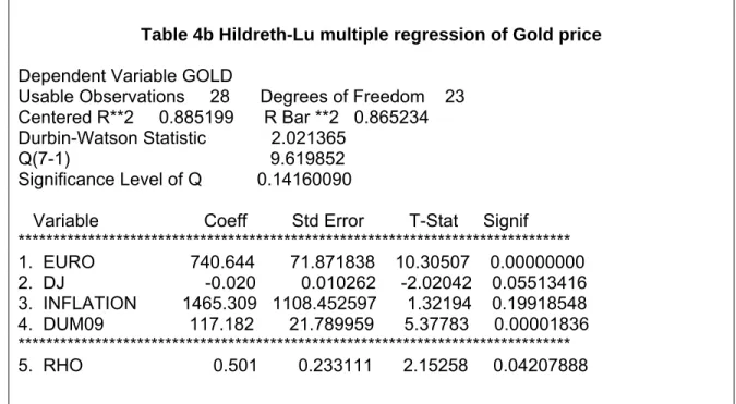
Table 4b Hildreth-Lu multiple regression of Gold price
Dependent Variable GOLD
Usable Observations 28 Degrees of Freedom 23 Centered R**2 0.885199 R Bar **2 0.865234 Durbin-Watson Statistic 2.021365
Q(7-1) 9.619852 Significance Level of Q 0.14160090
Variable Coeff Std Error T-Stat Signif ******************************************************************************* 1. EURO 740.644 71.871838 10.30507 0.00000000 2. DJ -0.020 0.010262 -2.02042 0.05513416 3. INFLATION 1465.309 1108.452597 1.32194 0.19918548 4. DUM09 117.182 21.789959 5.37783 0.00001836 ******************************************************************************* 5. RHO 0.501 0.233111 2.15258 0.04207888
With a DW now equal to 2, the autocorrelation coefficient is significant and changes the magnitude of the other coefficients:
the Euro coefficient has deceased to 740;
the correction for autocorrelation reduces the significance of inflation to the 20% level and forces inflation lagged by one period out of the regression;
there seems to exist a collinearity between DJ and inflation – stocks are used as a hedge against inflation.
22 The fact that gold price is negatively related to inflation lagged by one period could illustrate that it is not
However, the assumption of independence between some regressors and the error term is violated if there is collinearity or simultaneity. Therefore, the use of an instrumental variable regression such as 2SLS or GMM (Generalized Method of Moments) is necessary. In order to have a just identified model - where the number of instruments is equal to the number of free parameters to be estimated - the instruments chosen are DUM09 VXO INTEREST INFLATION
Table 5 Linear Regression - Estimation by GMM
Dependent Variable GOLD
Usable Observations 29 Degrees of Freedom 25 Durbin-Watson Statistic 1.662127
Variable Coeff Std Error T-Stat Signif ******************************************************************************* 1. EURO 963.922 66.025361 14.59928 0.00000000 2. DJ -0.053 0.009370 -5.69114 0.00000001 3. INFLATION 1280.167 525.889019 2.43429 0.01492094 4. DUM09 87.089 15.287461 5.69681 0.00000001
The effect of the GMM estimator is important since it reinforces the significance of the variables - all coefficients are significant at 1% level with the expected sign; the Euro coefficient now reaches a summit of 964 and the DJ coefficient is more than the double. Since the variables are not measured in the same units, it is difficult to judge which variable has the greatest impact on the gold price. However, by standardizing the value of the explanatory variables by the value of the price of gold (1000) on Oct 1st 2009and
multiplying these standardized values by their respective coefficients, we obtain EURO: 964x 0.00146 = 1.407
DJ: -0.053x 9.7 = -0.514 INFLATION: 1280x -0.00001 = -0.012 DUM09: 87x 0.001 = 0.087 ERROR = 0.032 GOLD PRICE (or TOTAL) 1.000
Although these results are not elasticity coefficients, it seems obvious that the two most important regressors are EURO and DJ, the contribution of the latter being almost three times less than the Euro coefficient in absolute value. Note that a decrease of the DJ has a positive impact on the price of gold.
Up to now the analysis has been conducted in terms of level instead of relative change of the variables. Except for the inflation variable that already measures the relative change of the price level, the other variables are transformed in log and, by taking the first differences, elasticity coefficients are obtained and are independent of the unit of measurement of variables –a prefix DL is added to each variable. The coefficient will now indicate which determinant has the greatest impact on variation of gold price.
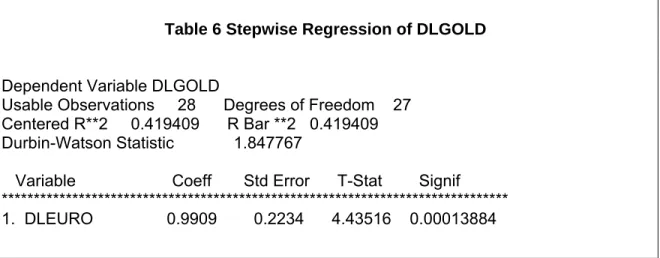
Table 6 Stepwise Regression of DLGOLD
Dependent Variable DLGOLD
Usable Observations 28 Degrees of Freedom 27 Centered R**2 0.419409 R Bar **2 0.419409 Durbin-Watson Statistic 1.847767
Variable Coeff Std Error T-Stat Signif ******************************************************************************* 1. DLEURO 0.9909 0.2234 4.43516 0.00013884
Contrary to the results obtained with variables in levels, there is only one variable that is significant when measured in relative change: it is Euro with an elasticity coefficient of unity. This shows again that the variation of the price of gold is directly linked with the variation of the value of the US Dollar. The value of the D-W stat (1.85) shows that the null hypothesis of autocorrelation is accepted.
On the other hand, a stepwise regression of DLEURO on the five other variables gives only two significant results: the variation of the price of gold and the variation of the Dow Jones index.
Table 7 Stepwise Regression of DLEURO
Dependent Variable DLEURO
Usable Observations 28 Degrees of Freedom 26 Centered R**2 0.513613 R Bar **2 0.494906 Durbin-Watson Statistic 2.537239
Variable Coeff Std Error T-Stat Signif
******************************************************************************* 1. DLGOLD 0.3937 0.0905 4.34819 0.00018768
2. DLDJ 0.1765 0.0787 2.24237 0.03368552
Although the Euro is rather inelastic to any of these two variables, the most interesting result is that the elasticity of Euro with respect to the price of gold is more than twice the elasticity with respect to DJ. This seems to confirm the existence of a simultaneous relation between Euro and the gold price. Note also the positive impact of the DJ on the Euro.
This is an interesting result and can explain the more complex relation between fear VXO, the DJ index, the Euro, and the gold price GOLD. We already observed from table 1 a negative correlation between a fear of deflation ΔVXO>0 and a fall of the stock exchange index ΔDJ<0. Econometric results from table 5 show a negative relation between the DJ and GOLD while results in table 7 show a positive link between DLEURO, DLGOLD and DLDJ. What happen if the fear of deflation falls or the fear of inflation rises? The fear of inflation is the negative of the fear of deflation. Therefore, we observe a sign change for DLVXO<0. Consequently,
DLVXO<0 → DLDJ>0 → DLGOLD<0 from table 5
DLDJ>0 → DLEURO>0 → DLGOLD>0 from tables 7 and 5.
Since the influence of Euro is about three times more important than the influence of the DJ index on the price of gold, the end result is that a fear of inflation has a positive impact on the price of gold.
The estimation of a two equation model by the GMM estimator -variables measured in levels- validates the results already obtained by OLS for the price of gold equation and the Euro equation. The coefficients have the same expected sign and they are all significant at a critical level of less than 2% with a reasonable DW.
Table 8 a) GMM estimation of the price of gold equation
Dependent Variable GOLD
Usable Observations 29 Degrees of Freedom 25 J-Specification(1) 1.758140
Significance Level of J 0.18485671 Durbin-Watson Statistic 1.642413
Variable Coeff Std Error T-Stat Signif *******************************************************************************
1. EURO 936.652 64.988781 14.41253 0.00000000 2. DJ -0.049 0.009211 -5.34712 0.00000009 3. INFLATION 1212.597 519.988152 2.33197 0.01970217 4. DUM09 87.758 15.293071 5.73847 0.00000001
b) GMM estimation of the Euro equation
Dependent Variable EURO
Usable Observations 29 Degrees of Freedom 25 J-Specification(1) 6.381521
Significance Level of J 0.01153146 Durbin-Watson Statistic 1.100718
Variable Coeff Std Error T-Stat Signif ******************************************************************************* 1. GOLD 0.0017 0.000065313 26.60197 0.00000000 2. VXO -0.0017 0.000834293 -2.06082 0.03932057 3. INTEREST 0.0437 0.027689110 1.57942 0.11424025 4. DUM09 -0.2103 0.038654830 -5.44287 0.00000005 Recall that that the best two significant variables in the DLEURO equation were DLGOLD and DLDJ with positive sign. A similar case is observed with the GMM estimator where the most significant variables are the price of gold and VXO with a negative sign for the latter. Since there is a negative correlation between VXO and DJ, it is another way of confirming the positive relation between Euro and DJ. The
interpretation is rather straightforward: an increase of fear of deflation pushes investors toward a safe haven – the US dollar. Note that the interest rate is positive but significant only at the 11% level. This result is contrary to expectation unless it sends a signal to the European central bank to raise their interest rate to protect their currency against
devaluation. Therefore, we have a simultaneous model which could be of the following form:
Gold = f( Euro, DJ, Inflation ) Euro = g( Gold,VXO, interest ).
4.5 Co-integration analysis
The results obtained above are based on the assumption that the series observed on gold price and Euro are stationary –no unit root- and the exogenous variables are non stochastic regressors. These assumptions must be abandoned after carrying unit root tests on all variables. Two unit root tests were carried:
Augmented Dickey-Fuller test with a constant and 4 lags and with critical value of -2.985 at 5% level;
Phillips-Perron test with a constant and a critical value of -2.966 at the 5% level. All variables except the interest rate have a unit root – they have a calculated t-value below the above critical values. The interest rate has a calculated t-value of -9.29 with the ADF test and -3.49 with the PP test.
Despite the small sample, a integration analysis was done by assuming one co-integration relation normalized with respect either to the price of gold or to the value of euro. The other variables are stochastic regressors, the variations of which are random shocks on the endogenous variable. Note that with 3 lags, we have only 7 degrees of freedom left.
Table 9 Error correction model with rank = 1
Sample: 1 to 29 (29 observations) Effective Sample: 4 to 29 (26 observations) Obs. - No. of variables: 7
System variables: GOLD VXO DJ INTEREST EURO INFLATION Constant/Trend: Unrestricted Constant
Lags in VAR: 3
THE EIGENVECTOR(s)(transposed)
GOLD VXO DJ INTEREST EURO INFLATION 0.021 0.056 0.002 5.050 -22.318 -68.273: BETA NORMALIZED WITH RESPECT TO EURO
-0.001 -0.002 -0.0001 -0.226 1.000 3.059 (-36.818) (-21.946) (-48.863) (-35.287) (.NA) (16.678) BETA NORMALIZED WITH RESPECT TO GOLD
1.000 2.667 0.095 240.476 -1056.190 -3251.095
Let us examine the results of the co-integration equation normalized with respect to gold price. There is a positive and significant link between Euro and gold price (1056.19). 23
Hence, the market value of the US dollar is significantly and directly linked to gold – a devaluation of the US dollar is directly reflected by an increase of the gold price. Note also a 10% increase in the magnitude of the coefficient when compared to the GMM estimation. Inflation is also positively and significantly related to gold price (3251). Note also an increase in magnitude of 150% of the coefficient when compared with the GMM
23 One should remember that a co-integration equation is a stationary linear combination of the form E[
β’Z] =E[e] = 0. Hence, except for the standardized variable, all other coefficients of explanatory variables should have an opposite sign when they are read as the right hand side of the equation.
result. A new feature is the significant negative relation between the interest rate and the price of gold (-240.5). This variable was excluded from the stepwise regression. This result is fully in accordance with our expectation: a substantial increase of the interest rate would raise the value of the US dollar, hence decrease the Euro and the gold price. As observed before, the DJ index is negatively related to gold price (-0.095). Note that the value of its coefficient has almost doubled when compared to the GMM result. Note also that a negative relation exists between the fear index and the price of gold (-2.667) – a fear of deflation would bring down the price of all commodities including gold as an ordinary commodity. It is interesting to note that this co-integration relation is well identified with the gold price and improve greatly the results obtained by other estimators.
Let’s turn now to the Euro standardized equation. Note that all the coefficients seem to be significant: gold and interest rate are positively related with Euro as in the previous GMM results. However, since VXO and DJ variables are negatively correlated, the change of sign of VXO is somewhat intriguing. The DJ coefficient remains positive as in the case of the GMM result. One way to have a better identification is to impose a priori restrictions on some coefficients of explanatory variables.
The estimation of a two equation model (GOLD and EURO) with two restrictions in each equation – in accord with the model specified at the end of section 4.4 - necessitates the specification of an Error Correction model of rank 2, that is two co-integration relations. Results contained in table 9 gives an even better identification.24
Table 9 Error correction model with rank = 2 and 2 restrictions
BETA(transposed)
GOLD EURO VXO DJ INTEREST INFLATION Beta(1) 1.000 -2136.264 0.000 0.132 0.000 -4529.446 (.NA) (-41.587) (.NA) (42.998) (.NA) (-27.438) Beta(2) 0.001 1.000 0.007 0.000 0.724 0.000 (12.387) (.NA) (18.796) (.NA) (56.070) (.NA)
The first co-integration relation is well identified to the gold price equation with significant coefficients and the latter have increased substantially with respect to the co-integration without restrictions: the magnitude of Euro coefficient (2136.3) has increased by more than 100%, the inflation coefficient (4529) has increased by 40%, and the magnitude of DJ coefficient (-0.132) has also increased by nearly 40%. Note also the great
improvement in the significance of the coefficients when compared with the GMM results.
The second co-integration is not so well identified with Euro since the gold price coefficient is negative (-0.001). There are however interesting results with the Euro equation: the interest rate coefficient is strongly negatively correlated with Euro - which was not the case before. These results seem to indicate the need to specify a more complex structure of interdependence between variables with the rank of the Π matrix most likely higher than 2. More research with more observations is required if one wants to continue this type of analysis.
4.6 Summary of econometric results
Before concluding, let us summarize our econometric results.
1. 85% of the variance of gold price is explained by one variable: EURO. Since the latter is defined with respect to the US dollar, the strong link between gold and the US dollar becomes obvious.
2. 60% of the variance of the interest rate is explained by inflation. Hence 40% remains unexplained. That gives an opportunity to other targeted variables of the monetary policy to play an independent role in the variation of the interest rate. 3. A stepwise regression of gold price on all explanatory variables shows that DJ
and inflation have a significant influence on gold price but their significance is small compared to Euro – they add only 1.5% to the explained variance of gold. When variables are measured in terms of proportional change, gold price has a unitary elasticity with Euro. The other variables are not significant. Hence, there is a one to one correspondence between gold price variations and US dollar variations!
4. If there is simultaneity between gold price and Euro, a stepwise regression of Euro on the other explanatory variables shows that only two variables come out