HAL Id: tel-01320380
https://tel.archives-ouvertes.fr/tel-01320380
Submitted on 23 May 2016
HAL is a multi-disciplinary open access archive for the deposit and dissemination of
sci-L’archive ouverte pluridisciplinaire HAL, est destinée au dépôt et à la diffusion de documents
Mirsad Buljubasic
To cite this version:
Mirsad Buljubasic. Efficient local search for several combinatorial optimization problems. Operations Research [cs.RO]. Université Montpellier, 2015. English. �NNT : 2015MONTS010�. �tel-01320380�
Préparée au sein de l’école doctorale
I2S - Information, Structures, Systèmes
et de l’unité de recherche
LGI2P - Laboratoire de Génie Informatique et d’Ingénierie de Production de l’école des mines d’Alès
Spécialité:
Informatique
Présentée par
Mirsad BULJUBAŠIĆ
Efficient local search for
several combinatorial
optimization problems
Soutenue le 20 novembre 2015 devant le jury composé de
M. Jin-Kao HAO, Professeur Rapporteur Université d’Angers
M. Mutsunori YAGIURA, Professeur Rapporteur Nagoya University
M. Miklos MOLNAR, Professeur Examinateur Université de Montpellier
M. Said HANAFI, Professeur Examinateur Université de Valenciennes et du Hainaut-Cambrésis
This thesis focuses on the design and implementation of local search based algorithms for discrete optimization. Specifically, in this research we consider three different problems in the field of combinatorial op-timization including "One-dimensional Bin Packing" (and two similar problems), "Machine Reassignment" and "Rolling Stock unit manage-ment on railway sites". The first one is a classical and well known op-timization problem, while the other two are real world and very large scale problems arising in industry and have been recently proposed by Google and French Railways (SNCF) respectively. For each problem we propose a local search based heuristic algorithm and we compare our results with the best known results in the literature. Additionally, as an introduction to local search methods, two metaheuristic approaches, GRASP and Tabu Search are explained through a computational study on Set Covering Problem.
Cette thèse porte sur la conception et l’implémentation d’algorithmes approchés pour l’optimisation en variables discrètes. Plus particulière-ment, dans cette étude nous nous intéressons à la résolution de trois problèmes combinatoires difficiles : le « Bin-Packing », la « Réaffecta-tion de machines » et la « GesRéaffecta-tion des rames sur les sites ferroviaires ». Le premier est un problème d’optimisation classique et bien connu, tandis que les deux autres, issus du monde industriel, ont été proposés respectivement par Google et par la SNCF. Pour chaque problème, nous proposons une approche heuristique basée sur la recherche locale et nous comparons nos résultats avec les meilleurs résultats connus dans la littérature. En outre, en guise d’introduction aux méthodes de recherche locale mise en œuvre dans cette thèse, deux métaheuristiques, GRASP et Recherche Tabou, sont présentées à travers leur application au problème de la couverture minimale.
Contents i
List of Figures vii
List of Tables ix
Introduction 1
1 GRASP and Tabu Search 7
1.1 Introduction . . . 8
1.2 General principle behind the method . . . 8
1.3 Set Covering Problem . . . 10
1.4 An initial algorithm . . . 12 1.4.1 Constructive phase . . . 12 1.4.2 Improvement phase . . . 14 1.5 Benchmark . . . 14 1.6 greedy(α)+descent experimentations . . . 15 1.7 Tabu search . . . 18
1.7.1 The search space . . . 18
1.7.2 Evaluation of a configuration . . . 18
1.7.3 Managing the Tabu list . . . 19
1.7.4 Neighborhood . . . 20
1.7.5 The Tabu algorithm . . . 20
1.8
greedy(α)+descent+Tabu
experimentations . . . 211.10 Conclusion . . . 24
2 One-dimensional Bin Packing 25 2.1 Introduction . . . 25 2.2 Relevant work . . . 29 2.2.1 BPP . . . 29 2.2.2 VPP . . . 31 2.3 A proposed heuristic . . . 31 2.3.1 Local Search . . . 33 2.3.1.1 Tabu search . . . 36 2.3.1.2 Descent procedure . . . 38
2.4 Discussion and parameters . . . 39
2.5 Applying the method on 2-DVPP and BPPC . . . 42
2.6 Computational results . . . 43
2.6.1 BPP . . . 43
2.6.2 2-DVPP . . . 49
2.6.3 BPPC . . . 51
2.7 Conclusion . . . 53
3 Machine Reassignment Problem 55 3.1 Introduction . . . 55
3.2 Problem specification and notations . . . 57
3.2.1 Decision variables . . . 57 3.2.2 Hard constraints . . . 57 3.2.2.1 Capacity constraints . . . 57 3.2.2.2 Conflict constraints . . . 58 3.2.2.3 Spread constraints . . . 58 3.2.2.4 Dependency constraints . . . 58
3.2.2.5 Transient usage constraints . . . 59
3.2.3 Objectives . . . 59
3.2.3.1 Load cost . . . 59
3.2.3.2 Balance cost . . . 59
3.2.3.4 Service move cost . . . 60
3.2.3.5 Machine move cost . . . 60
3.2.3.6 Total objective cost . . . 60
3.2.4 Instances . . . 61
3.3 Related work . . . 62
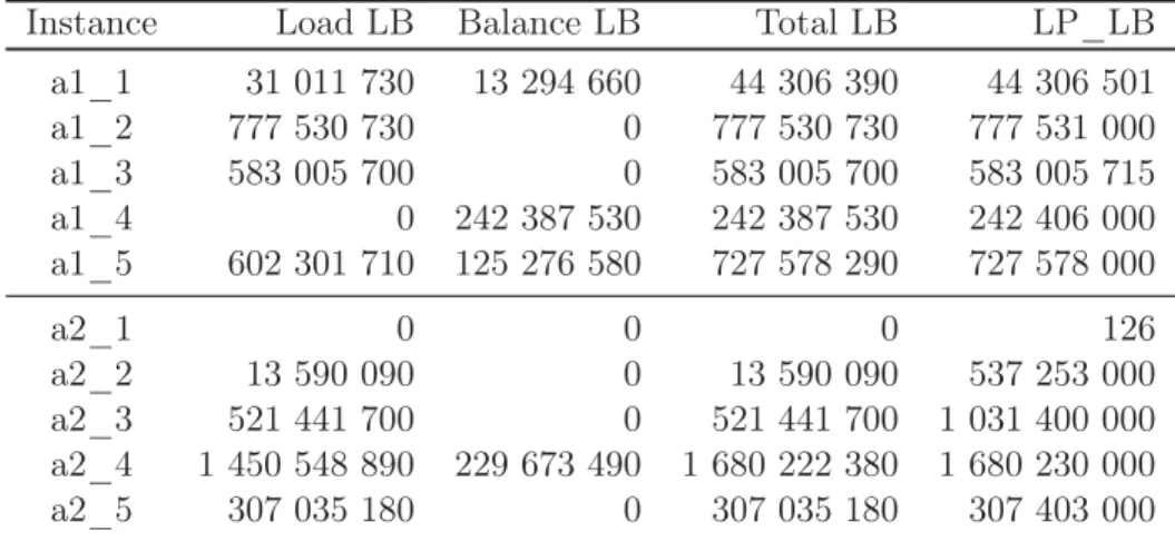
3.4 Lower Bound . . . 65
3.4.1 Load Cost Lower Bound . . . 65
3.4.2 Balance Cost Lower Bound . . . 66
3.5 Proposed Heuristic . . . 67
3.5.1 Neighborhoods . . . 68
3.5.1.1 Shift and Swap . . . 69
3.5.1.2 Big Process Rearrangement (BPR) Neighborhood . 74 3.5.2 Tuning the algorithm . . . 77
3.5.2.1 Neighborhoods exploration . . . 77
3.5.2.2 Sorting processes . . . 78
3.5.2.3 Noising . . . 79
3.5.2.4 Randomness - dealing with seeds and restarts . . . 80
3.5.2.5 Parameters . . . 82
3.5.2.6 Efficiency . . . 82
3.5.3 Final Algorithm . . . 85
3.6 Computational Results . . . 86
3.7 Conclusion . . . 88
4 SNCF Rolling Stock Problem 91 4.1 Introduction . . . 91 4.2 Problem Statement . . . 92 4.2.1 Planning horizon . . . 92 4.2.2 Arrivals . . . 93 4.2.3 Departures . . . 94 4.2.4 Trains . . . 96
4.2.4.1 Trains initially in the system . . . 97
4.2.4.2 Train categories . . . 97
4.2.5 Joint-arrivals and joint-departures . . . 99
4.2.6 Maintenance . . . 101
4.2.7 Infrastructure resources . . . 103
4.2.7.1 Transitions between resources . . . 103
4.2.7.2 Single tracks . . . 107
4.2.7.3 Platforms . . . 107
4.2.7.4 Maintenance facilities . . . 108
4.2.7.5 Track groups . . . 108
4.2.7.6 Yards . . . 109
4.2.7.7 Initial train location . . . 109
4.2.7.8 Imposed resource consumptions . . . 110
4.2.8 Solution representation . . . 111
4.2.9 Conflicts on track groups . . . 111
4.2.10 Objectives . . . 113
4.2.11 Uncovered arrivals/departures and unused initial trains . . . 113
4.2.12 Performance costs . . . 114
4.2.12.1 Platform usage costs . . . 114
4.2.12.2 Over-maintenance cost . . . 115
4.2.12.3 Train junction / disjunction operation cost . . . 115
4.2.12.4 Non-satisfied preferred platform assignment cost . . 115
4.2.12.5 Non-satisfied train reuse cost . . . 116
4.3 Related Work . . . 116
4.4 Two Phase Approach . . . 118
4.4.1 Simplifications . . . 118
4.4.2 Assignment problem . . . 119
4.4.2.1 Greedy assignment algorithm . . . 122
4.4.2.2 Greedy assignment + MIP . . . 124
4.4.2.3 Choosing maintenance days . . . 129
4.4.3 Scheduling problem . . . 133
4.4.3.1 Possible train movements . . . 134
4.4.3.2 General rules for choice of movements . . . 136
4.4.3.3 Resource consumption and travel feasibility . . . . 137
4.4.3.5 Travel starting time . . . 139
4.4.3.6 Choosing platforms and parking resources . . . 140
4.4.3.7 Dealing with yard capacity . . . 140
4.4.3.8 Choosing gates: Avoiding conflicts on track groups 141 4.4.3.9 Virtual visits . . . 143
4.4.3.10 Scheduling order . . . 144
4.4.4 Iterative Improvement Procedure . . . 145
4.4.4.1 Feasible to infeasible solution with more trains . . 145
4.4.4.2 Local search to resolve track group conflicts . . . . 146
4.4.5 Final Algorithm . . . 151
4.5 Evaluation and Computational results . . . 152
4.5.1 Benchmarks . . . 152
4.5.2 Evaluation and results . . . 153
4.6 Qualification version . . . 155
4.6.1 Assignment problem . . . 156
4.6.1.1 Greedy assignment algorithm . . . 158
4.6.1.2 MIP formulation for assignment . . . 158
4.6.1.3 Greedy assignment + matching + MIP . . . 160
4.6.2 Scheduling problem . . . 162
4.6.2.1 Choosing platforms, parking resources and travel starting times . . . 162
4.6.3 Evaluation and Computational results . . . 163
4.7 Conclusion . . . 164
Conclusions 167
1.1 Incidence matrix for a minimum coverage problem . . . 11
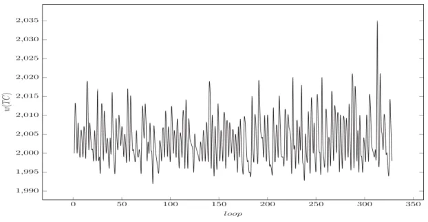
2.1 Fitness function oscillation . . . 40
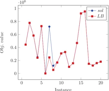
3.1 Gap between our best solutions and lower bounds on A and B datasets 68 3.2 Results with/without sorting processes and with/without noising . . 81
3.3 Objective function change during the search . . . 83
4.1 Junction of two trains . . . 99
4.2 Disjunction of two trains . . . 101
4.3 Example of resources infrastructure . . . 103
4.4 Infrastructure for instances A1 – A6 . . . 104
4.5 Infrastructure for instances A7 – A12 . . . 104
4.6 Example of gates in track group . . . 106
4.7 Example of resource with only one gate, on side A . . . 106
4.8 Conflicts in the same direction . . . 112
4.9 Objective parts importance . . . 117
4.10 Assignment graph . . . 121
4.11 Sorting Example . . . 129
4.12 Solution Process . . . 146
4.13 Objective function oscillation during improvement phase for in-stance B1 . . . 148
4.14 Objective function oscillation during improvement phase for in-stance X4. . . 149
1.1 Occurrences of solutions by z value for the S45 instance . . . 13
1.2 Improvement in z values for the S45 instance . . . 15
1.3 Characteristics of the various instances . . . 15
1.4 greedy(α)+descent results . . . 16
1.5 greedy(α)+descent+Tabu results . . . 22
1.6 greedy(1)+descent+Tabu results . . . 23
2.1 Results of exact approach based on Arc-Flow formulation . . . 45
2.2 Number of optimally solved instances when limiting the running time of the exact approach based on Arc-Flow formulation. . . 45
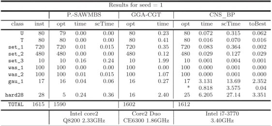
2.3 Results with a seed set equal to 1 . . . 46
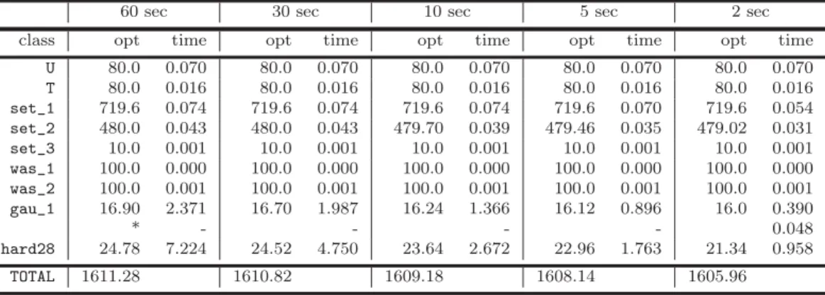
2.4 Average Results for 50 seeds with different time limits . . . 47
2.5 Detailed results for hard28 dataset . . . 49
2.6 Results with simplifications . . . 50
2.7 Two-dimensional Vector Packing results . . . 52
2.8 Cardinality BPP results . . . 52
3.1 The instances A . . . 62
3.2 The instances B . . . 63
3.3 Lower Bounds - instances A . . . 67
3.4 Lower Bounds - instances B . . . 67
3.5 Shift+Swap results . . . 73
3.6 Shift+Swap with randomness results . . . 74
3.7 Shift+Swap+BPR results . . . 76
3.9 Results obtained with sorting the processes . . . 79
3.10 Results for dataset A . . . 88
3.11 Results for datasets B and X . . . 89
4.1 Assignment values B . . . 128
4.2 First Feasible results on B instances . . . 145
4.3 Instances B characteristics . . . 152
4.4 Results on datasets B and X . . . 154
4.5 Uncovered arrivals/departures . . . 155
4.6 Assignment results for dataset A . . . 161
4.7 Dataset A characteristics . . . 163
1.1 GRASP procedure . . . 9 1.2 Randomized Greedy . . . 9 1.3 greedy(α) . . . 13 1.4 descent(x) . . . 14 1.5 GRASP1 . . . 16 1.6 updateTabu(j) . . . 19 1.7 evalH(j1, j2) . . . 20 1.8 tabu(x,N ) . . . 21 1.9 GRASP2 . . . 22 1.10 TABU . . . 23 2.1 Next Fit . . . 27 2.2 CN S_BP . . . 32 2.3 CN S() . . . 34 2.4 pack_set() . . . 36 2.5 T abuSearch() . . . 38 2.6 Descent() . . . 39 3.1 shift() . . . 71 3.2 fillShift() . . . 71 3.3 swap() . . . 72 3.4 fillSwap() . . . 72 3.5 BPR - one move . . . 75 3.6 NLS . . . 86 3.7 LS() . . . 86
4.1 Greedy assignment . . . 125
4.2 F inalAlgorithm . . . 151
Many problems in combinatorial optimization are NP-hard which implies that it is generally believed that no algorithms exist that solve each instance of such a problem to optimality using a running time that can be bounded by a polynomial in the instance size. As a consequence, much effort has been devoted to the design and analysis of algorithms that can find high quality approximative solutions in reasonable, i.e. polynomial, running times. Many of these algorithms apply some kind of neighborhood search and over the years a great variety of such local search algorithms have been proposed, applying different kinds of search strategies often inspired by optimization processes observed in nature.
Local search algorithms move from solution to solution in the space of candidate solutions (the search space) by applying local changes, until a solution deemed optimal is found or a time bound is elapsed. These algorithms are widely applied to numerous hard computational problems, including problems from computer science (particularly artificial intelligence), mathematics, operations research, en-gineering, and bioinformatics. For an introduction to local search techniques and their applications in combinatorial optimization, the reader is referred to the book edited by Aarts and Lenstra (Aarts and Lenstra [1997]).
This thesis focuses on the construction of effective and efficient local search based methods to tackle three combinatorial optimisation problems from different ap-plication areas. Two of these problems arise from real-world apap-plications where essential and complex features of problems are present. The first one is Machine Reassignment problem, defined by Google, and concerns optimal assignment of processes to machines i.e. improvement of the usage of a set of machines. The
second one is Rolling Stock Problem, defined by French Railways (SNCF), which can be classified as a scheduling (planning) problem. The task is to plan train movements in terminal stations between their arrival and departure. Both prob-lems have been proposed in ROADEF/EURO Challenge competitions in 2012 and 2014, which are international competitions jointly organized by French and Euro-pean societies of Operations Research. Although these two problems come from different application domains, they share some common features: (1) they are complex due to the presence of the large set of constraints which represent the real-world restrictions, e.g. logical restrictions, resources restrictions, etc. (2) they tend to be large. Due to these two main features of the problems, in general, solving these problems is computationally challenging. To tackle these problems efficiently, in this thesis we construct solution methods based on local search. Besides those two large scale problems, we present a local search method for ef-ficiently solving One-dimensional Bin Packing Problem (BPP), classical and well known combinatorial optimization problem. Even though the classical instances for BPP are of a significantly smaller size than those for previous two problems, solving BPP is computationally challenging as well. This is particularly due to the fact that (1) optimal solutions are usually required (in contrast to the two previously mentioned large scale problems where optimal solutions are usually not known) and (2) some of the instances are constructed in order to be "difficult". Additionally, as an introduction to local search methods, a computational study for solving Set Covering problem by GRASP and Tabu Search is presented. Methods developed for solving Set Covering, Bin Packing and Machine Reas-signment problems are pure local search approaches, meaning that local search starts from initial solutions already given (in case of Machine Reassignment) or constructed in a very simple way (First Fit heuristic for Bin Packing and sim-ple heuristic for Set Covering). On the other hand, for Rolling Stock problem, approach combines local search with greedy heuristics and Mixed Integer Pro-gramming (MIP). Greedy heuristic (rather complex) and Integer ProPro-gramming have been used in order to obtain initial feasible solutions to the problem, which are then the subject of an improvement procedures based on local search. MIP has been used in order to produce better initial solutions (combined with greedy
pro-cedure). Nevertheless, high quality solutions can be produced even when omitting the MIP part, as was the case in our solution submitted to the ROADEF/EURO Challenge 2014 competition. Proposed local search approaches for Bin Packing and SNCF Rolling Stock problems are applied on partial configurations (solutions). This local search on a partial configuration is called the Consistent Neighborhood Search (CNS) and has been proven efficient in several combinatorial optimization problems (Habet and Vasquez[2004]; Vasquez et al.[2003]). CNS has been intro-duced in Chapter 1 as an improvement procedure in GRASP method for solving Set Covering Problem.
Our goal was to develop effective local search algorithms for the considered prob-lems, which are capable of obtaining high quality results in a reasonable (often very short) computation time. Since complexity of the local search methods is mainly influenced by the complexity (size) of the local search neighborhoods, we tried to use simple neighborhoods when exploring the search space. Additional elements had to be included in the strategies in order to make them effective. The most important among those possible additional features are the intensification of the search, applied in those areas of the search space that seem to be particularly appealing, and the diversification, in order to escape from poor local minima and move towards more promising areas. Key algorithm features leading to high qual-ity results will be explained, in a corresponding chapter, for each of the considered problems.
This thesis is organized into four main chapters:
1. GRASP and Tabu Search: Application to Set Covering Problem This chapter presents the principles behind the GRASP (Greedy Random-ized Adaptive Search Procedure) method and details its implementation in the aim of resolving large-sized instances associated with a hard combinato-rial problem. The advantage of enhancing the improvement phase has also been demonstrated by adding, to the general GRASP method loop, a Tabu search on an elementary neighborhood.
to solving the one-dimensional bin packing problem (BPP) has been pre-sented. This local search is performed on partial and consistent solutions. Promising results have been obtained for a very wide range of benchmark instances; best known or improved solutions obtained by heuristic methods have been found for all considered instances for BPP. This method is also tested on vector packing problem (VPP) and evaluated on classical bench-marks for two-dimensional VPP (2-DVPP), in all instances yielding optimal or best-known solutions, as well as for Bin Packing Problem with Cardinality constraints.
3. Machine Reassignment Problem The Google research team formalized and proposed the Google Machine Reassignment problem as a subject of ROADEF/EURO Challenge 2012. The aim of the problem is to improve the usage of a set of machines. Initially, each process is assigned to a machine. In order to improve machine usage, processes can be moved from one machine to another. Possible moves are limited by constraints that address the com-pliance and the efficiency of improvements and assure the quality of service. The problem shares some similarities with Vector Bin Packing Problem and Generalized Assignment Problem.
We proposes a Noisy Local Search method (NLS) for solving Machine Reas-signment problem. The method, in a round-robin manner, applies the set of predefined local moves to improve the solutions along with multiple starts and noising strategy to escape the local optima. The numerical evaluations demonstrate the remarkable performance of the proposed method on MRP instances (30 official instances divided in datasets A, B and X) with up to 50,000 processes.
4. SNCF Rolling Stock Problem We propose a two phase approach com-bining mathematical programming, greedy heuristics and local search for the problem proposed in ROADEF/EURO challenge 2014, dedicated to the rolling stock management on railway sites and defined by French Railways (SNCF). The problem is extremely hard for several reasons. Most of induced sub–problems are hard problems such as assignment problem, scheduling problem, conflicts problem on track groups, platform assignment problem,
etc. In the first phase, a train assignment problem is solved with a com-bination of a greedy heuristic and mixed integer programming (MIP). The objective is to maximize the number of assigned departures while respecting technical constraints. The second phase consists of scheduling the trains in the station’s infrastructure while minimizing number of cancelled (uncov-ered) departures, using a constructive heuristic. Finally, an iterative pro-cedure based on local search is used to improve obtained results, yielding significant improvements.
GRASP and Tabu Search:
Application to Set Covering
Problem
This chapter will present the principles behind the GRASP (Greedy Randomized Adaptive Search Procedure) method and offer a sample application to the Set Covering problem. The advantage of enhancing the improvement phase has also been demonstrated by adding, to the general GRASP method loop, a Tabu search on an elementary neighborhood.
Resolution of the set covering problem by GRASP mathod presented here has been inspired by the work ofFeo and Resende[1995]. The method presented inFeo and Resende[1995] has been modified by adding a tabu search procedure to the general GRASP method loop. This tabu search procedure that works with partial solu-tion (partial cover) is referred as Consistent Neighborhood Search (CNS) and has been proven efficient in several combinatorial optimization problems (Habet and Vasquez [2004];Vasquez et al. [2003]). The search is performed on an elementary neighborhood and makes use of an exact tabu management.
Most of the method features can be found in the literature (in the same or sim-ilar form) and, therefore, we do not claim the originality of the work presented herein; this chapter serves mainly as an introduction to GRASP and Tabu search metaheuristics and Consistent Neighborhood Search procedure. Also, application
to Set Covering problem showed to be suitable due to the simplicity of the method proposed and results obtained on difficult Set Covering instances.
1.1
Introduction
The GRASP (Greedy Randomized Adaptive Search Procedure) method generates several configurations within the search space of a given problem, based on which it carries out an improvement phase. Relatively straightforward to implement, this method has been applied to a wide array of hard combinatorial optimiza-tion problems, including: scheduling Binato et al. [2001], quadratic assignment Pitsoulis et al. [2001], the traveling salesman Marinakis et al. [2005], and main-tenance workforce scheduling Hashimoto et al. [2011]. One of the first academic papers on the GRASP method is given in Feo and Resende[1995]. The principles behind this method are clearly described and illustrated by two distinct imple-mentation cases: one that inspired the resolution in this chapter of the minimum coverage problem, the other applied to solve the maximum independent set prob-lem in a graph. The interested reader is referred to the annotated bibliography by P. Festa and M.G.C. Resende Festa and Resende [2002], who have presented nearly 200 references on the topic.
Moreover, the results output by this method are of similar quality to those deter-mined using other heuristic approaches like simulated annealing, Tabu search and population algorithms.
1.2
General principle behind the method
The GRASP method consists of repeating a constructive phase followed by an improvement phase, provided the stop condition has not yet been met (in most instances, this condition corresponds to a computation time limit expressed, for ex-ample, in terms of number of iterations or seconds). Algorithm1.1below describes the generic code associated with this procedure.
Algorithm 1.1: GRASP procedure
input : α, random seed, time limit.
1 repeat
2 X ← Randomised Greedy(α); 3 X ← Local Search(X, N); 4 if z(X) better than z(X∗) then 5 X∗← X;
6 untilCPU time> time limit;
step of assigning the current variable - and its value - is slightly modified so as to generate several choices rather than just a single one at each iteration. These potential choices constitute a restricted candidate list (or RCL), from which a candidate will be chosen at random. Once the (variable, value) pair has been established, the RCL list is updated by taking into account the current partial configuration. This step is then iterated until obtaining a complete configuration. The value associated with the particular (variable, value) pairs (as formalized by the heuristic function H), for still unassigned variables, reflects the changes intro-duced by selecting previous elements. Algorithm1.2summarizes this configuration construction phase, which will then be improved by a local search (simple descent, tabu search or any other local modification-type heuristic). The improvement phase is determined by the neighborhood N implemented in an attempt to refine the solution generated by the greedy algorithm.
Algorithm 1.2: Randomized Greedy
input: α , random seed.
1 X = {∅}; 2 repeat
3 Assemble the RCL on the basis of heuristic H and α; 4 Randomly select an element xh from the RCL; 5 X = X ∪ {xh};
6 Update H;
7 untilconfigurationX has been completed ;
The evaluation of heuristic function H serves to determine the insertion of (variable, value) pairs onto the RCL (restricted candidate list). The way in which this criterion is taken into account exerts considerable influence on the behavior exhibited during the constructive phase: if only the best (variable, value) pair is
selected relative to H, then the same solution will often be obtained, and iterating the procedure will be of rather limited utility. If, on the other hand, all possible candidates were to be selected, the random algorithm derived would be capable of producing quite varied configurations, yet of only mediocre quality: the likelihood of the improvement phase being sufficient to yield good solutions would thus be remote. The size of the RCL therefore is a determinant parameter of this method. From a pragmatic standpoint, it is simpler to manage a qualitative acceptance threshold (i.e. H(xj) better than α × H∗, where H∗ is the best benefit possible and
α is a coefficient lying between 0 and 1) for the random drawing of a new (variable, value) pair to be assigned rather than implement a list of k potential candidates, which would imply a data sort or use of more complicated data structures. The terms used herein are threshold-based RCL in the case of an acceptance threshold and cardinality-based RCL in all other cases.
The following sections will discuss in greater detail the various GRASP method components through an application to set covering problem.
1.3
Set Covering Problem
Given a matrix (with m rows and n columns) composed solely of 0′s and 1′s,
the objective is to identify the minimum number of columns such that each row contains at least one 1 in the identified columns. One type of minimum set covering problem can be depicted by setting up an incidence matrix with the column and row entries shown below (Figure 1.1).
More generally speaking, an n-dimensional cost vector is to be considered, containing strictly positive values. The objective then consists of minimizing the total costs of columns capable of covering all rows: this minimization is known as the Set Covering Problem, as exemplified by the following linear formulation:
cover = 0 1 1 1 0 0 0 0 0 1 0 1 0 1 0 0 0 0 1 1 0 0 0 1 0 0 0 0 0 0 0 1 1 1 0 0 0 0 0 1 0 1 0 1 0 0 0 0 1 1 0 0 0 1 1 0 0 0 0 0 0 1 1 0 1 0 0 0 0 1 0 1 0 0 1 0 0 0 1 1 0 1 0 0 1 0 0 1 0 0 0 1 0 0 1 0 0 1 0 0 0 1 0 0 1 0 0 1
Figure 1.1: Incidence matrix for a minimum coverage problem
min z = n X j=1 costj× xj ∀i ∈ [1, m] n X j=1 coverij × xj ≥ 1, ∀j ∈ [1, n] xj ∈ {0, 1}. (1.1)
For 1 ≤ j ≤ n, the decision variable xj equals 1 if column j is selected, and 0
otherwise. In the case of Figure1.1 for example, x =< 101110100 > constitutes a solution whose objective value z is equal to 5.
If costj equals 1 for each j, then the problem becomes qualified as a Unicost
Set Covering Problem, as stated at the beginning of this section. Both the Unicost Set Covering Problem and more general Set Covering Problem are classified as combinatorial NP-hard problems Garey and Johnson [1979]; moreover, once such problems reach a certain size, their resolution within a reasonable amount of time becomes impossible by means of exact approaches. This observation justifies the implementation of heuristics approaches, like the GRASP method, to handle these instances of hard problems.
1.4
An initial algorithm
This section will revisit the same algorithm proposed by T. Feo and M.G.C. Re-sende in one of their first references on the topic Feo and Resende [1995], where the GRASP method is applied to the Unicost Set Covering problem. It will then be shown how to improve results and extend the study to the more general Set Covering problem through combining GRASP with the T abu search metaheuristic.
1.4.1 Constructive phase
Let x be the characteristic vector of all columns X (whereby xj = 1 if column j
belongs to X and xj = 0 otherwise): x is the binary vector of the mathematical
model in Figure1.1. The objective of the greedy algorithm is to produce a config-uration x with n binary components, whose corresponding set X of columns covers all the rows. Upon each iteration (out of a total n), the choice of column j to be added to X (xj = 1) will depend on the number of still uncovered rows that this
column covers. As an example, the set of columns X = {0, 2, 3, 4, 6} corresponds to the vector x =< 101110100 >, which is the solution to the small instance shown in Figure 1.1.
For a given column j, we hereby define the heuristic function H(j) as follows:
H(j) =
( C(X∪{j})−C(X)
costj if xj = 0
C(X\{j})−C(X)
costj if xj = 1
where C(X) is the number of rows covered by the set of columns X. The list of RCL candidates is managed implicitly: H∗ = H(j) maximum is first calculated
for all columns j such that xj = 0. The next step calls for randomly choosing
a column h such that xh = 0 and H(h) ≥ α × H∗. The pseudo-code of the
randomized greedy algorithm is presented below in Algorithm1.3.
The heuristic function H(), which determines the insertion of columns into the RCL, is to be reevaluated at each step so as to take into account only the uncovered rows. This is the property that gives rise to the adaptive nature of the GRASP method.
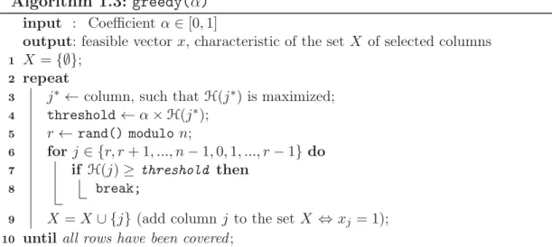
Algorithm 1.3: greedy(α)
input : Coefficient α ∈ [0, 1]
output: feasible vector x, characteristic of the set X of selected columns
1 X = {∅}; 2 repeat
3 j∗← column, such that H(j∗) is maximized; 4 threshold ← α × H(j∗);
5 r ← rand() modulo n;
6 for j ∈ {r, r + 1, ..., n − 1, 0, 1, ..., r − 1} do 7 if H(j) ≥ threshold then
8 break;
9 X = X ∪ {j} (add column j to the set X ⇔ xj = 1); 10 until all rows have been covered;
corresponds to data file data.45 (renamed S45), which has been included in the four Unicost Set Covering problems, as derived from Steiner’s triple systems and accessible on J.E. Beasley’s OR-Library site J.E.Beasley [1990]. By setting the values 0, 0.2, . . . 1 for α and 1, 2, . . . 100 for the seed of the pseudo-random sequence, the results table presented in Table 1.1 has been obtained. This table lists the
α\z 30 31 32 33 34 35 36 37 38 39 40 41 total 0.0 0 0 0 0 0 1 9 10 15 17 21 15 88 0.2 0 0 0 1 3 15 34 23 18 5 1 0 100 0.4 0 0 0 5 13 30 35 16 1 0 0 0 100 0.6 0 2 2 45 38 13 0 0 0 0 0 0 100 0.8 0 11 43 46 0 0 0 0 0 0 0 0 100 1.0 0 55 19 26 0 0 0 0 0 0 0 0 100
Table 1.1: Occurrences of solutions by z value for the S45 instance
number of solutions whose coverage size z lies between 30 and 41. The quality of these solutions is clearly correlated with the value of parameter α. For the case α = 0 (random assignment), it can be observed that the greedy() function produces 12 solutions of a size that strictly exceeds 41. No solution with an optimal coverage size of 30 (known for this instance) is actually produced.
1.4.2 Improvement phase
The improvement algorithm proposed by T. Feo and M.G.C. Resende Feo and Resende[1995] is a simple descent on an elementary neighborhood N. Let x denote the current configuration, then a configuration x′ belongs to N (x) if a unique j
exists such that xj = 1 and x′j = 0 and moreover that ∀i ∈ [1, m]
Pn
j=1coverij×
x′
j ≥ 1. Between two neighboring configurations x and x′, a redundant column
(from the standpoint of row coverage) was deleted. Algorithm 1.4: descent(x)
input : characteristic vector x from the set X output: feasible x without any redundant column
1 while redundant columns continue to exist do
2 Find redundant j ∈ X such that costj is maximized; 3 if j exists then
4 X = X \ {j}
Pseudo-code 1.4 describes this descent phase and takes into account the cost of each column, with respect to the column deletion criterion, for subsequent application to the more general Set Covering problem.
Moreover, the same statistical study on the occurrences of the best solutions to the greedy() procedure on its own (see Table 1.1) is repeated, this time with addition of the descent() procedure, yielding the results provided in Table1.2. A leftward shift is observed in the occurrences of objective value z; such an observa-tion effectively illustrates the benefit of this improvement phase. Before pursuing the various experimental phases, the characteristics of our benchmark will first be presented.
1.5
Benchmark
The benchmark used for experimentation purposes is composed of fourteen in-stances made available on J.E. Beasley’s OR-Library site J.E.Beasley [1990].
The four instances data.45, data.81, data.135 and data.243 (renamed re-spectively S45, S81,S135 and S243) make up the test datasets in the reference
α\z 30 31 32 33 34 35 36 37 38 39 40 41 total 0.0 0 0 0 0 1 9 10 15 17 21 15 8 96 0.2 0 0 1 3 15 34 23 18 5 1 0 0 100 0.4 0 0 5 13 30 35 16 1 0 0 0 0 100 0.6 2 2 45 38 13 0 0 0 0 0 0 0 100 0.8 11 43 46 0 0 0 0 0 0 0 0 0 100 1.0 55 19 26 0 0 0 0 0 0 0 0 0 100
Table 1.2: Improvement in z values for the S45 instance
Inst. n m Inst. n m Inst. n m
G1 10000 1000 H1 10000 1000 S45 45 330
G2 10000 1000 H2 10000 1000 S81 81 1080 G3 10000 1000 H3 10000 1000 S135 135 3015 G4 10000 1000 H4 10000 1000 S243 243 9801 G5 10000 1000 H5 10000 1000
Table 1.3: Characteristics of the various instances
article by T. Feo and M.G.C. Resende Feo and Resende [1995]: these are all Uni-cost Set Covering problems. The ten instances G1...G5 and H1...H5 are considered Set Covering problems. Table1.3 indicates, for each test dataset, the number n of columns and number m of rows.
The GRASP method was run 100 times for each of the three α coefficient values of 0.1, 0.5 and 0.9. Seed g of the srand(g) function assumes the values 1, 2, . . . , 100. For each method execution, the CPU time is limited to 10 seconds. The computer used for this benchmark is equipped with an i7 processor running at 3.4GHz with 8 gigabytes of hard drive memory. The operating system is a Linux, Ubuntu 12.10.
1.6
greedy(α)+descent experimentations
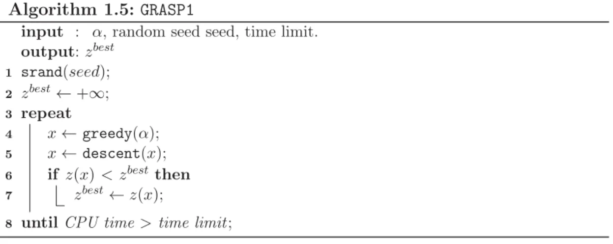
Provided below is the pseudo-code of the initial GRASP method version, GRASP1, used for experimentation on the fourteen datasets of our benchmark.
Algorithm 1.5: GRASP1
input : α, random seed seed, time limit. output: zbest 1 srand(seed); 2 zbest← +∞; 3 repeat 4 x ← greedy(α); 5 x ← descent(x); 6 if z(x) < zbest then 7 zbest← z(x);
8 until CPU time > time limit;
those of the Numerical Recipes Press et al. [1992]. Moreover, let’s point out that the coding of the H function is critical: introduction of an incremental computation is essential to obtaining relative short execution times. The values given in Table
1.4 summarize the results output by the GRASP1 procedure. The primary results
α = 0.1 α = 0.5 α = 0.9 Inst. z∗ z # P zg 100 z # P zg 100 z # P zg 100 G1 176 240 1 281.83 181 1 184.16 183 3 185.14 G2 154 208 1 235.34 162 7 164.16 159 1 160.64 G3 166 199 1 222.59 175 2 176.91 176 3 176.98 G4 168 215 1 245.78 175 1 177.90 177 5 178.09 G5 168 229 1 249.40 175 1 178.56 174 6 175.73 H1 63 69 1 72.30 67 29 67.71 67 5 68.19 H2 63 69 2 72.28 66 1 67.71 67 1 68.51 H3 59 64 1 68.80 62 1 64.81 63 34 63.66 H4 58 64 1 67.12 62 18 62.86 63 80 63.20 H5 55 61 1 62.94 59 2 60.51 57 99 57.01 S45 30 30 100 30.00 30 100 30.00 30 100 30.00 S81 61 61 100 61.00 61 100 61.00 61 100 61.00 S135 103 104 2 104.98 104 4 104.96 103 1 104.10 S243 198 201 1 203.65 203 18 203.82 203 6 204.31
Table 1.4: greedy(α)+descent results tables provided herein indicate the following:
• the name of the tested instance,
• for each value of coefficient α = 0.1, 0.5 and 0.9:
– the best value z found using the GRASP method,
– the number of times # this value has been reached per 100 runs, – the average of the 100 values produced by this algorithm.
For the four instances S, the value displayed in column z∗ is optimal (Ostrowski
et al. [2011]). On the other hand, the optimal value for the other ten instances (G1,. . . ,G5 and H1,. . . ,H5) remains unknown: the z∗ values for these ten instances
are the best values published in the literature ( Azimi et al.[2010]; Caprara et al. [1999];Yagiura et al. [2006]).
With the exception of instance S243, the best results are obtained using the values 0.5 and 0.9 of RCL management parameter α. For the four instances derived from Steiner’s triple problem, the values published by T. Feo and M.G.C. ResendeFeo and Resende[1995] are corroborated. However, when compared with the works of Z. Naji-Azimi et al. Azimi et al. [2010], performed in 2010, or even those of A. Caprara et al. Caprara et al. [1998], dating back to 2000, these results prove to be relatively far from the best published values.
1.7
Tabu search
This section will focus on adding a Tabu search phase to the GRASP method in order to generate more competitive results with respect to the literature. The algorithm associated with this Tabu search is characterized by:
• an infeasible configuration space S, such that z(x) < zmin,
• a simple move (of the 1-change) type, • a strict Tabu list.
1.7.1 The search space
In relying on the configuration x0 output by the descent phase (corresponding to
a set X of columns guaranteeing row coverage), the Tabu search will explore the space of configurations x with objective value z(x) less than zmin = z(xmin), where
xmin is the best feasible solution found by the algorithm. The search space S is
thus formally defined as follows:
S= x ∈ {0, 1}n/ z(x) < z(xmin)
1.7.2 Evaluation of a configuration
It is obvious that the row coverage constraints have been relaxed. The H evaluation function of a column j now contains two components:
H1(j) = ( C(X ∪ {j}) − C(X) if xj = 0 C(X \ {j}) − C(X) if xj = 1 and H2(j) = ( costj if xj = 0 −costj if xj = 1
This step consists of repairing the coverage constraints (i.e. maximizing H1)
1.7.3 Managing the Tabu list
This task involves use of the Reverse Elimination Method proposed by F. Glover and M. Laguna (Glover and Laguna[1997]), which has been implemented in order to exactly manage the Tabu status of potential moves: a move is forbidden if and only if it leads to a previously encountered configuration. This Tabu list is referred to as a strict list. Algorithm 1.6: updateTabu(j) input : j ∈ [0, n − 1] 1 running list[iter] = j; 2 i ← iter; 3 iter ← iter + 1; 4 repeat 5 j ← running list[i]; 6 if j ∈ RCS then 7 RCS ← RCS/{j}; 8 else 9 RCS ← RCS ∪ {j}; 10 if |RCS| = 1 then 11 j = RCS[0] is tabu; 12 i ← i − 1 13 until i < 0;
The algorithm we describe herein is identical to that successfully run on another combinatorial problem with binary variables Nebel [2001]. The running list is actually a table in which a recording is made, upon each iteration, of the column j targeted by the most recent move: xj = 0 or xj = 1. This column is considered the
move attribute. The RCS (for Residual Cancellation Sequence) is another table in which attributes will be either added or deleted. The underlying principle consists of reading one by one, from the end of the running list, past move attributes, in adding RCS should they be absent and removing RCS if already present. The following equivalence is thus derived: |RCL| = 1 ⇔ RCL[0] prohibited. The interested reader is referred to the academic article by F. Dammeyer and S. Voss Dammeyer and Voß [1993] for further details on this specific method.
1.7.4 Neighborhood
We have made use of an elementary 1-change move: x′ ∈ N(x) if ∃!j/x′
j 6= xj. The
neighbor x′ of configuration x only differs by one component yet still satisfies the
condition z(x′) < zmin, where zmin is the value of the best feasible configuration
identified. Moreover, the chosen non-Tabu column j minimizes the hierarchical criterion ((H1(j), H2(j))). Pseudo-code 1.7 describes the evaluation function for
this neighborhood.
Algorithm 1.7: evalH(j1, j2)
input : column interval [j1, j2] output: best column identified j∗ 1 j∗← −1; 2 H∗ 1 ← −∞; 3 H∗ 2 ← +∞; 4 for j1 ≤ j ≤ j2 do 5 if j non tabu then
6 if (xj = 1) ∨ (z + costj < zmin) then 7 if (H1(j) > H∗ 1) ∨ (H1(j) = H∗1 ∧ H2(j) < H∗2) then 8 j∗← j; 9 H∗ 1 ← H1(j); 10 H∗ 2 ← H2(j);
1.7.5 The Tabu algorithm
The general Tabu() procedure uses as an argument the solution x produced by the descent() procedure, along with a maximum number of iterations N . Rows
6 through 20 of Algorithm 1.8 correspond to a search diversification mechanism. Each time a feasible configuration is produced (i.e. |X| = m), the value zmin is
updated and the Tabu list is reset to zero.
The references to rows 2and 20will be helpful in explaining the algorithm in Section1.9.
Algorithm 1.8: tabu(x,N )
input : feasible solution x, number of iterations N output: zmin, xmin
2 2 zmin← z(x) ; 3 iter ← 0 ; 4 repeat 6 6 r ← rand() modulo n; 8 8 j∗ ← evalH(r, n − 1); 10 10 if j∗ < 0 then 12 12 j∗ ← evalH(0, r − 1); 13 if xj∗ = 0 then 14 add column j∗; 15 else 16 remove column j∗; 17 if |X| = m then 18 zmin ← z(x) ; 20 20 xmin← x ; 21 iter ← 0;
22 delete the Tabu status ; 23 updateTabu(j∗);
24 until iter ≥ N or j∗< 0;
1.8
greedy(α)+descent+Tabu
experimentations
For this second experimental phase, the benchmark is similar to that discussed in Section 1.6. Total CPU time remains limited to 10 seconds, while the maximum number of iterations without improvement for the Tabu() procedure equals half the number of columns for the treated instance (i.e.n/2). The pseudo-code of the GRASP2 procedure is specified by Algorithm 1.9.
Table 1.5 effectively illustrates the significant contribution of the Tabu search to the GRASP method. All z∗ column values are found using this version of the
GRASP method. In comparison with Table1.4, parameter α is no longer seen to exert any influence on results. It would seem that the multi-start function of the GRASP method is more critical to the Tabu phase than control over the RCL candidate list. However, as will be demonstrated in the following experimental phase, it still appears that rerunning the method, under parameter α control, does play a determinant role in obtaining the best results.
Algorithm 1.9: GRASP2
input : α, random seed seed, time limit. output: zbest 1 zbest← +∞; 2 srand(seed); 3 repeat 4 x ← greedy(α); 5 x ← descent(x); 6 z ← Tabu(x, n/2); 7 if z < zbest then 8 zbest← z;
9 until CPU time > time limit;
α = 0.1 α = 0.5 α = 0.9 Inst. z∗ z # P zg 100 z # P zg 100 z # P zg 100 G1 176 176 100 176.00 176 96 176.04 176 96 176.04 G2 154 154 24 154.91 154 32 155.02 154 57 154.63 G3 166 167 4 168.46 167 10 168.48 166 1 168.59 G4 168 168 1 170.34 170 35 170.77 170 29 170.96 G5 168 168 10 169.59 168 7 169.66 168 10 169.34 H1 63 63 11 63.89 63 2 63.98 63 5 63.95 H2 63 63 21 63.79 63 13 63.87 63 5 63.95 H3 59 59 76 59.24 59 82 59.18 59 29 59.73 H4 58 58 99 58.01 58 98 58.02 58 100 58.00 H5 55 55 100 55.00 55 100 55.00 55 100 55.00 S45 30 30 100 30.00 30 100 30.00 30 100 30.00 S81 61 61 100 61.00 61 100 61.00 61 100 61.00 S135 103 103 49 103.51 103 61 103.39 103 52 103.48 S243 198 198 100 198.00 198 100 198.00 198 100 198.00
Table 1.5: greedy(α)+descent+Tabu results
1.9
greedy(1)+Tabu
experimentations
To confirm the benefit of this GRASP method, let’s now observe the behavior of Algorithm 1.10: TABU. For each value of the pseudo-random function rand() seed (1 ≤ g ≤ 100 for the call-up of srand()), a solution is built using the greedy(1) procedure, whereby redundant x columns are deleted in allowing for completion of the Tabu(x,n) procedure, provided CPU time remains less than 10 seconds.
Inst. z # P zg 100 Inst. z # P zg 100 Inst. z # P zg 100 G1 176 95 176.08 H1 63 2 63.98 S45 30 100 30.00 G2 154 24 155.22 H2 63 4 63.96 S81 61 100 61.00 G3 167 19 168.48 H3 59 36 59.74 S135 103 28 103.74 G4 170 3 171.90 H4 58 91 58.09 S243 198 98 198.10 G5 168 20 169.39 H5 55 97 55.03
Table 1.6: greedy(1)+descent+Tabu results
For this final experimental phase, row 2 has been replaced in pseudo-code
1.8 by zmin ← +∞. Provided the CPU time allocation has not been depleted,
the Tabu() procedure is reinitiated starting with the best solution it was able to produce during the previous iteration. This configuration is saved in row 20. Moreover, the size of the running list is twice as long.
Algorithm 1.10: TABU
input : random seed, time limit. output: zbest 1 zbest← +∞; 2 srand(seed); 3 x ← greedy(1); 4 xmin← descent(x); 5 repeat 6 x ← xmin; 7 z, xmin ← Tabu(x, n); 8 if z < zbest then 9 zbest← z;
10 until CPU time > time limit;
In absolute value terms, these results fall short of those output by Algorithm
1.9: GRASP2. This TABU version has produced values of 167 and 170 for instances G3 and G4 vs. 166 and 168 respectively for the GRASP2 version. Moreover, the majority of average values are of poorer quality than those listed in Table 1.5.
1.10
Conclusion
This chapter has presented the principles behind the GRASP method and has de-tailed their implementation in the aim of resolving large-sized instances associated with a hard combinatorial problem. Section 1.4.1 exposed the simplicity involved in modifying the greedy heuristic proposed by T.A. Feo and M.G.C. Resende, namely:
H(j) = (
C(X ∪ {j}) − C(X) if xj = 0
C(X \ {j}) − C(X) if xj = 1
in order to take into account the column cost and apply the construction phase, not only to the minimum coverage problem, but to the Set Covering Problem as well.
The advantage of enhancing the improvement phase has also been demon-strated by adding, to the general GRASP method loop, a Tabu search on an elementary neighborhood.
One-dimensional Bin Packing
In this chapter we study the One-dimensional Bin Packing problem (BPP) and present efficient and effective local search algorithm for solving it.
2.1
Introduction
Given a set I = {1, 2, . . . , n} of items with associated weights wi (i = 1, . . . , n),
the bin packing problem (BPP) consists of finding the minimum number of bins, of capacity C, necessary to pack all the items without violating any of the capacity constraints. In other words, one has to find a partition of items {I1, I2, . . . , Im}
such that
X
i∈Ij
wi ≤ C, j = 1, . . . , m
and m is minimum. The bin packing problem is known to be NP-hard (Garey and Johnson[1979]). One of the most extensively studied combinatorial problems, BPP has a wide range of practical applications such as in storage allocation, cutting stock, multiprocessor scheduling, loading in flexible manufacturing systems and many more. The Vector Packing problem (VPP) is a generalization of BPP with multiple resources. Item weights wr
i and bin capacity Cr are given for each resource
r ∈ {1, . . . , R} and the following constraint has to be respected: X
i∈Ij
wr
Bin packing problem with cardinality constraints (BPPC) is a bin packing problem where, in addition to capacity constraints, an upper bound k ≥ 2 on the number of items packed into each bin is given. This constraint can be expressed as:
X
i∈Ij
1 ≤ k, j = 1, . . . , m
Obviously, bin packing with cardinality constraints can be seen as a two dimen-sional vector packing problem where C2 = k and wi1 = w2i = 1 for each item
i ∈ 1, . . . , n.
Without loss of generality we can assume that capacities and weights are integer in each of the defined problems.
We will present a new improvement heuristic based on a local search for solv-ing BPP, VPP with two resources (2-DVPP) and BPPC. The method will first be described in detail for a BPP problem, followed by the set of underlying adapta-tions introduced to solve the 2-DVPP and BPPC.
A possible mathematical formulation of BPP is minimize z = n X i=1 yi (2.1) subject to z = n X j=1 wjxij ≤ Cyi, i ∈ N = {1, 2, . . . , n} (2.2) n X i=1 xij = 1, j ∈ N (2.3) yi ∈ {0, 1}, i ∈ N (2.4) xij ∈ {0, 1}, i, j ∈ N, (2.5) where
yi = 1 if bin i is used, otherwise yi = 0;
Definition 1 For a subset S ⊆ I, we let w(S) =P
i∈Swi.
Some of the most simple algorithms for solving BPP are given in the following discussion.
Next Fit Heuristic (NF) works as follows: Place the items in the order in which they arrive. Place the next item into the current bin if it fits. Otherwise, create a new bin. Pseudo code is given in Algorithm2.1.
This algorithm can waste a lot of bin space, since the bins we close may not be very full. However, it does not require memory of any bin except the current one. One should be able to improve the performance of the algorithm by considering previous bins that might not be full. Similar to NF are First Fit Heuristic (FF), Best Fit Heuristic (BF), and Worst Fit Heuristic (BF). First Fit works as follows: Place the items in the order in which they arrive. Place the next item into the lowest numbered bin in which it fits. If it does not fit into any open bin, create a new bin. Best Fit and Worst Fit heuristics are similar to FF, but instead of placing an item into the first available bin, the item is placed into the bin with smallest (greatest for WF) remaining capacity it fits to.
If it is permissible to preprocess the list of items, significant improvements are Algorithm 2.1: Next Fit
1 Input: A set of all items I, wi≤ C, ∀i ∈ I;
2 Output: A partition {Bi} of I where w(Bi) ≤ C for each i; 3 b ← 0; 4 foreach i ∈ I do 5 if wi+ w(Bb) ≤ C then 6 Bb ← Bb∪ {i} 7 else 8 b ← b + 1; 9 Bb ← {i}; 10 return B1, . . . , Bb;
possible for some of the heuristic algorithms. For example, if the items are sorted before they are packed, a decreasing sort improves the performance of both the First Fit and Best Fit algorithms. This two algorithms are refered to as First Fit Decreasing (FFD) and Best Fit Decreasing. Johnson[1973] showed that F F D
heuristic uses at most 11/9×OP T +4 bins, where OP T is the the optimal solution (smallest number of bins) to the problem.
In our proposed heuristic, the solution is iteratively improved by decreasing the number of bins being utilized. The procedure works as follows. First, the upper bound on the solution value, U B, is obtained by a variation of First Fit (FF) heuristic. Next, an attempt is made to find a feasible solution with U B − 1 bins, and this process continues until reaching lower bound, the time limit or maximum number of search iterations. Aside from the simple lower bound, lPni=1wi
C
m
, lower bounds developed byFekete and Schepers[2001],Martello and Toth[1990] (bound L3) and Alvim et al.[2004] have also been used.
In order to find a feasible solution with a given number of bins, m < U B, a local search is employed. As opposed to the majority of work published on BPP, a local search explores partial solutions that consist of a set of assigned items without any capacity violation and a set of non-assigned items. Moves consist of rearranging both the items assigned to a single bin and non-assigned items, i.e. adding and dropping items to and from the bin. The objective here is to minimize the total weight of non-assigned items. This local search on a partial configura-tion is called the Consistent Neighborhood Search and has been proven efficient in several combinatorial optimization problems (Habet and Vasquez [2004]; Vasquez et al.[2003]). Therefore, our approach will be refered as CNS_BP in the reminder of the chapter.
An exploration of this search space of partial solutions comprises two parts, which will be run in succession: 1) a tabu search with limited add/drop moves and 2) a descent with a general add/drop move. This sequence terminates when a com-plete solution has been found or the running time limit (or maximum number of iterations) has been exceeded.
Additionally, the algorithm makes use of a simple reduction procedure that con-sists of fixing the assignments of all pairs of items that fill an entire bin. More precisely, s set of item pairs (i, j) such that wi+ wj = C has been identified, and
This same reduction has been used in the majority of papers on BPP. It is im-portant to mention that not using reduction procedure will not have a significant influence on the final results (but can speed up the search) and, moreover, no reduction is possible for a big percentage of the instances considered.
This chapter will be organized as follows. Section 2.2 will address relevant work, and our approach will be described in Section2.3. The general framework will be presented first, followed by a description of all algorithmic components. A number of critical remarks and parameter choices will be discussed in Section2.4. Section
2.5presents a summary of methodological adaptations to 2-DVPP and BPPC. The results of extensive computational experiments performed on the available set of instances, for BPP, 2-DVPP and BPPC will be provided in Section 2.6, followed by conclusions drawn in the final section.
2.2
Relevant work
2.2.1 BPP
A large body of literature relative to one-dimensional bin packing problems is avail-able. Both exact and heuristic methods have been applied to solving the problem. Martello and Toth[1990] proposed a branch-and-bound procedure (MTP) for solv-ing the BPP.Scholl et al.[1997] developed a hybrid method (BISON) that combines a tabu search with a branch-and-bound procedure based on several bounds and a new branching scheme. Schwerin and Wäscher [1999] offered a new lower bound for the BPP based on the cutting stock problem, then integrated this new bound into MTP and achieved high-quality results. de Carvalho[1999] proposed an exact algorithm using column generation and branch-and-bound.
Gupta and Ho [1999] presented a minimum bin slack (MBS) constructive heuristic. At each step, a set of items that fits the bin capacity as much as possible is identified and packed into the new bin. Fleszar and Hindi [2002] developed a hybrid algorithm that combines a modified version of the MBS and the Variable Neighborhood Search. Their hybrid algorithm performed very well in computa-tional experiments, having obtained the optimal solution for 1329 out of the 1370
instances considered.
Alvim et al. [2004] presented a hybrid improvement heuristic (HI_BP) that uses tabu search to move the items between bins. In their algorithm, a complete yet infeasible configuration is to be repaired through a tabu search procedure. Simple "shift and swap" neighborhoods are explored, in addition to balancing/unbalancing the use of bin pairs by means of solving a Maximum Subset Sum problem. HI_BP performed very well, as evidenced by finding optimal solutions for all 1370 bench-mark instances considered by Fleszar and Hindi [2002] and a total of 1582 out of the 1587 optimal solutions on an extensively studied set of benchmark instances. In recent years, several competitive heuristics have been presented with results similar to those obtained by HI_BP. Singh and Gupta [2007] proposed a com-pound heuristic (C_BP), in combining a hybrid steady-state grouping genetic algorithm with an improved version of Fleszar and Hindi’s Perturbation MBS. Loh et al.[2008] developed a weight annealing (WA) procedure, by relying on the concept of weight annealing to expand and accelerate the search by creating dis-tortions in various parts of the search space. The proposed algorithm is simple and easy to implement; moreover, these authors reported a high quality performance, exceeding that of the solutions obtained by HI_BP.
Fleszar and Charalambous[2011] offered a modification to the Perturbation-MBS method (Fleszar and Hindi[2002]) that introduces a new sufficient average weight (SAW) principle to control the average weight of items packed in each bin (referred to as Perturbation-SAWMBS). This heuristic has outperformed the best state-of-the-art HI_BP, C_BP and WA algorithms. Authors also presented corrections to the results that were reported for the WA heuristic, obtaining significantly lower quality results comparing to those reported in Loh et al. [2008].
To the best of our knowledge, the most recent work in this area, presented by (Quiroz-Castellanos et al. [2015]), entails a grouping genetic algorithm (GGA-CGT) that outperforms all previous algorithms in terms of number of optimal solutions found, particularly with a set of most difficult instances hard28.
Brandão and Pedroso [2013] devised an exact approach for solving bin packing and cutting stock problems based on an Arc-Flow Formulation of the problem;
these authors made use of a commercial Gurobi solver to process their model. They were able to optimally solve all standard bin packing instances within a reasonable computation time, including those instances that have not been solved by any heuristic method.
2.2.2 VPP
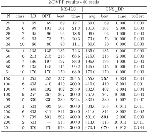
As regards the two-dimensional VPP, Spieksma [1994] proposed a branch-and-bound algorithm, while Caprara and Toth [2001] forwarded exact and heuristic approaches as well as a worst-case performance analysis. A heuristic approach using set-covering formulation was presented by Monaci and Toth [2006]. Masson et al. [2013] proposed an iterative local search (ILS) algorithm for solving the Machine Reassignment Problem and VPP with two resources; they reported the best results on the classical VPP benchmark instances of Spieksma (1994) and Caprara and Toth (2001).
2.3
A proposed heuristic
This section will describe our improvement heuristic. General improvement pro-cess is given in Algorithm2.2. Algorithm starts with applying a simple reduction procedure and constructing initial (feasible and complete) solution by applying FF heuristic on a randomly sorted set of items. This initial solution, containing U B bins, is then to be improved by a local search based procedure, which represents the core element of our proposal. More precisely, an attempt is made to find a complete solution with m = U B − 1 bins by applying local search on a partial solution, and this process continues until reaching lower bound, the time limit or maximum number of iterations (precisely defined later).
The remainder of a section will describe a procedure aimed at finding a feasible solution with a given number of bins, m. The inherent idea here is to build a partial solution with m − 2 bins and then transform it into a complete feasible solution with m bins through applying a local search. The partial solution is one that contains a set of items assigned to m − 2 bins, without any capacity violation, and
Algorithm 2.2: CN S_BP
1 remove item pairs (i, j) such that wi+ wj= C; 2 compute lower bound LB;
3 random shuffle the set of items; 4 m ← upper bound by First Fit;
5 while m > LB ∧ time limit not exceeded do 6 m ← m − 1;
7 create partial solution S with m − 2 bins; 8 CN S(S);
9 returnthe last complete solution;
a set of non-assigned items. The goal of the local search is, by rearranging the items, to obtain a configuration such that non-assigned items can be packed into two bins, thus producing a feasible solution with m bins.
One can notice that termination of the search by finding a complete solution, i.e. packing non-assigned items into two bins is not possible if more than two "big" items (with weight greater than or equal to half of the bin capacity) are non-assigned. Therefore, maximum number of non-assigned big items is limited to two during the whole procedure. When packing non-assigned items into two bins is possible, complete solution is obtained by simply adding the two new bins to the current set of bins.
Partial solution with m − 2 bins is built by deleting three bins from the last complete solution i.e. by removing all the items from these three bins and adding them to the set of non-assigned items (note that last feasible solution contains m + 1 bins). Bins to be deleted are selected in the following way:
• select the last two bins from a complete solution,
• select the last bin (excluding the last two) such that total number of non-assigned "big" items does not exceed two.
The capacity of all bins is never violated at any time during the procedure. Items have been randomly sorted before applying FF in order to avoid solutions with many small or many big non-assigned items, which could make the search more difficult or slower (this is the case, for example, if items are sorted in de-creasing order). This very same procedure is then used for all types of instances,
e.g. the same initial solution, same parameters, same order of neighborhood ex-ploration.
For the sake of simplicity, let’s assume that the non-assigned items are packed into the special bin with unlimited capacity, called trash can and denoted by T C. Let B = {b1, b2, . . . , bm−2} be the set of currently utilized bins, IB ⊆ I the set
of items assigned to the bins in B and Ib the set of items currently packed into
bin b ∈ B. Analogously, let IT C denote the set of currently non-assigned items.
Total weight and cardinality of a set of items S will be denoted by w(S) and |S| respectively. For the sake of simplicity, total weight and current number of items currently assigned to bin b ∈ B∪T C will be denoted by w(b) = w(Ib) and |b| = |Ib|.
2.3.1 Local Search
The Local Search procedure is applied to reach a complete solution with m bins, in starting from a partial one with m−2 bins constructed as described before. Several neighborhoods are explored during the search, which consists of two procedures executed in succession until a stopping criterion is met. These two procedures are: a) tabu search procedure and b) hill climbing/descent procedure. All moves consist of swapping the items between a bin in B and trash can T C.
Formally speaking, the local search moves include:
1. Swap(p, q) - consists of swapping p items from a bin b ∈ B with q items from T C,
2. P ack(b) - consists of optimally rearranging the items between bin b ∈ B and trash can T C, such that the remaining capacity in b is minimized, whereby a set of items (packing) P ⊆ Ib∪ IT C that fits the bin capacity as optimally
as possible is determined. P ack is a generalization of a Swap move with p and q both being unlimited.
Only the moves not resulting in any capacity violation are considered during this search. Swap move is used only in the tabu search procedure, while descent proce-dure makes use of a Pack move exclusively. Pseudo code of the proceproce-dure is given in Algorithm2.3and two main parts, TabuSearch() and Descent() procedures, will
be explained below in the corresponding sections.
Before explaining each of the two main parts of the local search, we will discuss Algorithm 2.3: CN S()
1 input: partial solution currSol;
2 while time or iterations limit not exceeded and complete solution not found do 3 currSol ← T abuSearch(currSol);
4 currSol ← Descent(currSol); 5 returncurrSol;
the search neighborhoods, objective function and search termination conditions. The goal of the local search procedure is to optimize the following lexicographic fitness function:
1. minimize the total weight on non-assigned items (minimize use of the trash can) : min w(T C);
2. maximize the number of items in the trash can: max |T C|.
The first objective is quite natural, while the second one is introduced in order to yield items with lower weights in the trash can, as this could: 1) increase the chance of terminating the search; and/or 2) enable a wider exploration of the search space. Formally, the following fitness function is to be minimized
obj(T C) = n × w(T C) − |T C| (2.6) The maximum number of items from the same bin that can be rearranged in a single Swap move is limited to three. More precisely, Swap(p, q) moves with
(p, q) ∈ {(0, 1), (1, 1), (2, 1), (1, 2), (2, 2), (2, 3), (3, 2)}
have been considered. Swap(0, 1) corresponds to shif t move, which consists of shifting (or adding) the item from the trash can to bin b ∈ B. All other possi-ble moves such as Swap(1, 0), Swap(0, 2) and Swap(3, 1) have been omitted since they increase the complexity of the neighborhood evaluation without improving the final results. The results obtained by not allowing more than two items from
a single bin to be swapped ((p, q) ∈ {(0, 1), (1, 1), (2, 1), (1, 2), (2, 2)}) will also be reported. Note that the higher complexity of these Swap(p, q) moves, with respect to the classical shift and swap moves used in the literature, is compensated by the fact that no moves between pairs of bins in B are performed.
Generating optimal packing for a set of items is a common procedure intro-duced in several papers (Gupta and Ho [1999], Fleszar and Hindi [2002], Fleszar and Charalambous [2011]) and originally proposed in Gupta and Ho[1999]. The P ack move is the same as the "load unbalancing" used in Alvim et al. [2004]. A Packing problem is equivalent to the Maximum Subset Sum (MSS) problem and can be solved exactly, for instance by either dynamic programming or enumera-tion. Let’s note that the packing procedure is only being used for a small subset of items, i.e. the set of items belonging to a single bin b ∈ B or trash can T C. Let pack_set(S) denote the solution to the MSS problem, which is a feasible subset P ⊆ S (whose sum of weights does not exceed C) with maximum total weight. The enumeration procedure has been used herein to solve the packing problem and pseudo code is given in Algorithm 2.4. Clearly, the complexity of the enumeration procedure is O(2l), where l is a number of considered items. The structure of
the available instances makes this approach reasonable, though a simple dynamic programming procedure of complexity O(l × C), can, if necessary, also be used. As mentioned before, no more than two "big" items (with weights greater than or equal to C/2) are allowed to be assigned to the trash can during the entire solving procedure. This is easily achieved by forbidding all Swap and Pack moves that result in having three or more big items in the trash can, but is omitted in the presented algorithms (pseudo-codes) for the simplicity reasons.
During the search, each time the total weight in the trash can is less than or equal to 2C, an attempt is undertaken to pack all items from the trash can into the two bins. This step involved simply uses the same P ack procedure, with quite
Algorithm 2.4: pack_set()
1 input: set of items S = {i1, . . . , ik}, current packing P (initialized to empty set); 2 output: best packing P∗(initialized to empty set);
3 if S 6= ∅ then 4 if w(P ) + wi 1 ≤ C then 5 pack_set(S \ {i1}, P ∪ {i1}); 6 pack_set(S \ {i1}, P ); 7 else 8 if (w(P ) > w(P∗)) ∨ (w(P ) = w(P∗) ∧ |P | < |P∗|) then 9 P∗← P
obviously packing into two bins being possible (feasible) if and only if
w(pack_set(IT C)) ≥ w(T C) − C. (2.7)
If packing into two bins is indeed possible, then the procedure terminates. Aside from the lower bound and time limit termination criteria, the procedure terminates when total number of solutions with w(T C) ≤ 2C obtained during the search exceeds a given number. Terminating the search after failing to pack non-assigned items into two bins too many times seems to be reasonable and this limit is set to 100000 for all considered instances. On the other hand, further ex-ploration of the search space does not look promising if solution with w(T C) ≤ 2C cannot be obtained in a reasonable time. Therefore, we also decide to terminate the search if no solution with w(T C) ≤ 2C has been found during the first ten algorithm loops (Tabu + Descent).
2.3.1.1 Tabu search
The main component of the improvement procedure is a tabu search that includes Swap moves between trash can and bins in B. In each iteration of the search, all swap moves between trash can and each bin have been evaluated and the best non-tabu move relative to the defined objective ( minimizing trash can use) is per-formed. Should two or more moves with the same objective exist, then a random choice is made. Note that the best move is carried out even if it does not improve