Inverse method to estimate air flow rate during free cooling using PCM-air heat exchanger

HAL Id: hal-01902272

https://hal.archives-ouvertes.fr/hal-01902272

Submitted on 23 Oct 2018

HAL is a multi-disciplinary open access archive for the deposit and dissemination of sci-entific research documents, whether they are pub-lished or not. The documents may come from teaching and research institutions in France or abroad, or from public or private research centers.

L’archive ouverte pluridisciplinaire HAL, est destinée au dépôt et à la diffusion de documents scientifiques de niveau recherche, publiés ou non, émanant des établissements d’enseignement et de recherche français ou étrangers, des laboratoires publics ou privés.

Inverse method to estimate air flow rate during free

cooling using PCM-air heat exchanger

A. Ousegui, B. Marcos, Michel Havet

To cite this version:

A. Ousegui, B. Marcos, Michel Havet. Inverse method to estimate air flow rate during free cooling using PCM-air heat exchanger. Applied Thermal Engineering, Elsevier, 2019, 146, pp.432 - 439. �10.1016/j.applthermaleng.2018.10.008�. �hal-01902272�

Inverse method to estimate air flow rate during free cooling using PCM-air

heat exchanger

A. Ouseguia *, B. Marcosb, M. Havetc

a _{Matériaux et Energies Renouvelables (EMER) Département de physique, Faculté des sciences de Meknès, BP}

11201, Avenue Zitoune, Meknès, Maroc

b_{Département de génie chimique et de génie biotechnologique Faculté de génie Université de Sherbrooke}

Québec J1K 2R, Canada

c_{ONIRIS, CNRS, GEPEA, UMR 6144,44322 Nantes, France}

Abstract

Free cooling technique using Phase Change Material (PCM) is a promising process to shave the peak load for the cooling system and reduce energy ventilation consumption. However it needs additional energy for the fan. In the way optimize the process we then proposed a first approach to estimate a priori the flow rate required to reach full freezing or thawing of PCM which is a useful indication of the process efficiency. The approach is based on the inverse method associated with sensitivity coefficient. The objective function was defined in terms of air temperature at the exit of the heat exchanger. The model was compared to experimental data, and the validation of numerical results shows the robustness and the consistency of this method. In the worst case, relative error does not exceed 510-03.

Key words: free cooling, conjugate heat transfer, inverse method, PCM-air heat exchanger Nomenclature

cp specific heat capacity (J/kg/K) e pcm thickness (m)

er relative error

*_{corresponding author. Tel.: +2126 02 47 29 75.}

H air gap thikness (m) J objective function

k thermal conductivity (W/m/K) L length of PCM and air gap (m) Lfrezzing latent heat for freezing PCM (J/kg) Lthawing latent heat for PCM fusion (J/kg) lf liquid fraction Q flow rate (m3/s) s sensitivity coefficient sf solid fraction T temperature (K) t time (s) u velocity (m/s) x horizontal coordinate (m) y vertical coordinate (m)

T sensitivity variable or temperature difference between measured and calculated

u sensitivity velocity variable Greek symbols  density (kg/m3) Ω boundary surface Ω computational domain δ Dirac distribution Subscribts

char charging regime disch discharging regime exp Experiment

f fluid or final time

in Inlet meas Measured s Solid 0 Initial 1 PCM domain 2 air domain

1 Introduction

Not only economical aspects, but also environmental concerns such as global warming and resources scarcity, urge researchers to look for other alternative for procurement (Renewable Energy) and/or rationalization (Energy efficiency) of energy. In the building sector, the energy consumption accounts for about 40% the world’s share of global energy consumption [1]. Among others, ventilation and air conditioning equipments consume almost 15% of this

total energy [2]. In order to address such an issue and subsequently shave the peak load for the cooling system, the free cooling technique coupled with the Phase Change Material (PCM) such as a Thermal Energy Storage (TES) system has been considered as an excellent alternative for cooling applications and overcoming overheating problems in buildings [3]. The free cooling concept harness the abundant atmospheric cool energy during the night in PCM to exploit this stored energy during the daytime, hence reaching the desired room comfort conditions. Indeed, due to his latent heat a PCM unit could save 38% of the building’s ventilation bill [4]. Such systems require the energy supply only for operating the fan, and this is more advantageous in comparison to mechanical cooling [5].The design consists of incorporating alternating slides of PCM and air gap in the building –generally on the roof- leading then to a plan or U heat exchanger. This process could be accomplished in two stages [6]:

Charging procedure (Figure 1-a): During the nighttime, the outdoor air temperature

is lower than ambient room temperature. The PCM is in the liquid state. As long as the cool outdoor air is circulating through the duct, it absorbs heat from the PCM (release of energy). Consequently the PCM will start to solidify by reaching the fusion temperature. Once the outdoor-indoor temperature variation is in the vicinity of zero the procedure is interrupted.

Discharging procedure (Figure 1-b): When the PCM is in a solid state; hot indoor air

circulates back across the unit and extracts cold stored in the PCM. The room temperature is then being reduced. The PCM starts to melt as a consequence of the absorption of the heat from the air.

Research on PCM and its integration in the building industry has attracted more interest during last 30 years. Zalba et al. [7] and Regin et al. [8] did a review on the works done on the classification of PCMs, their long-term stability, thermophysical properties and encapsulation technique. Tyagi et al. [9], Sharma et al. [10] and Sun et al.[11] outlined studies on thermal performance of various types of TES systems integrated into PCM including Trombe wall, wallboards, shutters, PCM building blocks, air-based heating systems, floor heating and ceiling boards.

Regarding the use of PCMs in the roofs of the buildings to generate heat exchanger Iten et al [12], Sharifi and Yamagata [13] shortlisted experimental works accomplished in this field, alongside different design configurations and their performance in proposed climatic conditions. Recently experimental researchers have conducted intense investigations to improve the performance of this technique. Medrano et al [14] compared experimentally average thermal power during melting and solidification of five small heat exchangers working as latent heat thermal storage systems. In this study commercial paraffin RT35 was used as PCM and water was used as heat transfer fluid. The study showed that compact heat

Figure 1 Principle of the bfree cooling system process [6]

Cold outdoor air circulated in PCM storage Fee or forced ventilation

Indoor air circulated in PCM storage

exchanger (CompHX-PCM) is by and large the one with the highest average thermal power (above 1 kW). However for average power per unit area and per average temperature gradient, results show that the double pipe heat exchanger with the PCM embedded in a graphite matrix (DPHX-PCM matrix) was proven to show a superior quality Reyes et al [15], designed a heat exchanger for solar energy accumulation, composed of soft drink cans filled with paraffin wax as PCM and mixed with aluminum wool to double the thermal conductivity. Experiments showed that the accumulated energy of 3 MJ, allows the temperature of 3.5 m3/h air flow rate to increase from 20 to 40°C during a period of 2 hours. Namura et al [16] use a mixed composition of sugar alcohol (Erythritol) as a PCM to improve the performance of a direct-contact heat exchanger. The study was focused on the effect of the height of PCM slab, the flow rate of heat transfer fluid (oil in this case), and the number of injection-nozzle holes on the performance of the process. They concluded that the increased number of injection-nozzle holes is positively correlated to the uniformity of the temperature in heat transfer fluid and liquid PCM. The heat exchanger designed by Labat et al [17] contains PCM to store enough energy and replace a 1kW heat pump during 2 hours. Eight airflow rates were conducted, for each one, temperature and air velocity were measured and heating power was calculated. Results showed that the stored and released energies are higher than 2kWh. This is a good indication that the optimization of the heat transfers is necessary in order to avoid a quick and a non-homogeneous heat transfer observed within the PCM attributed to free convection occurring in liquid phase of PCM. To improve the free cooling in the office building, Jaworsky [18] developed special ceilings made of gypsum mortar and micro-encapsulated phase change material (Micronal). Some experimental works reveal the necessity to associate a numerical model to experiments especially concerning the uniformity of the process and reaching the complete fusion (Discharging) or freezing (Charging) of PCM. The major difficulties of the numerical studies reside in the complexity of the free

cooling phenomenon because it involves a phase change phenomenon in PCM, conjugate heat transfer between heat transfer fluid (air in general) and PCM, evaluation of velocity field of fluid, and the non linearity of equations due to thermal dependent properties (mainly specific heat capacity of PCM). Many works conducted in this field can be classified according to parameters cited above. Al-saadi et al [19] and Tittelen et al [20] compared different schemes used in literature to simulate phase change in PCM. Studies show that apparent specific heat capacity is sensitive to melting range temperatures, however, for a given experimental data of apparent specific heat capacity this technique is suitable and gives satisfactory results [21]. Works focused on the performance of a heat exchanger (mainly the temperature field inside PCM and the air gap) that can be classified in two main categories: Analytical method ([16] and [22]) is based on hypothesis and simplifications so that the set of equations can be solved analytically. The latter category adopts the numerical methods using commercial or homemade software ([23], [24], [25], [26], [27], [28]). Simulations consider, in general, only heat conduction in PCM, convection and conduction in air (as fluid heat transfer). In general the velocity was considered constant except for Jaworski et al [27] where 1D steady Navier-Stokes equation was added to estimate the velocity field. Other works studied heat transfer behavior in a heat exchanger (air and PCM) and its effect on the ambient temperature (Room, Office…) ([29], [30], [31], [32]). The obtained results in the level of the heat exchanger were

linked to zonal software (like TRNSYS) to ascend to ambient room temperature. These types of studies are time consuming (simulation for weeks or months) and even they give global information of the performance of the free cooling technique; the accuracy of these studies is then compromised.

Despite the increasing interest into the free cooling technique, especially during the last decade, many technical tools and design improvement are required for its commercialization in the building sector. Both experimental and numerical researches have

been conducted to unravel parameters influencing this kind of process. Thambidurai et al [33] pointed out that the PCM temperature range, geometry of the PCM container, inlet air temperature, encapsulation thickness and the air flow rate are the main parameters affecting the free cooling performance. The control of this last factor ensures full solidification of the PCM during the charging stage or complete melting during discharging. Arkar et al ([34]-[35]) recommended that air flow rate during the charging process should be three to four times higher than air flow rates during the discharging process. Zalba et al [36] and Saman et al [37] observed however that a higher air flow rate boosts the heat transfer rate and leads to a shortened time phase change in both steps. However while charging, if the air temperature is not less than the subcooling temperature of the PCM, a higher air flow rate is not beneficial according to Waqas and Kumar [38].

Cold outdoor air circulates in the building, via natural or forced ventilation. Even the first type is less energy consumer, but it suffers on some limitations [39]. Firstly, natural ventilation effectiveness depends much on outside wind environment, (3 m/s is generally required for obvious cooling). Secondly, natural ventilation is not suitable in rainy days with opening windows or when outside air is dirty or hot for better quality and thermal comfort.

In the other side, the whole use of mechanical ventilation increases building energy consumption, and sometimes may induce occupant-health problem. This requires a rationalization of the use of forced ventilation, taking into account quality and thermal comfort requirements.

We believe that the value of the airflow rate in a building is driven by the necessity of air change and thermal comfort (maximum and minimum temperature). Then, there is a range of possible values, which makes optimization study complicated. More, once the model is developed the validation should be on optimal experiment. Another possible solution, is to

develop a numerical model based on inverse method. Such approach can be easily validated with the abundance of experimental work existing in literature. And later add the parameters constraint to the objective function.

The main objective of this paper is to propose an inverse method based on sensitivity coefficient technique to estimate during the free cooling in both charging and discharging regimes, the air flow-rate required to fit the desired exit path temperature accurately;. Taking into account specific thermal heat capacity dependency and hysteresis phenomenon related to freezing and thawing PCM. Once the method is validated with existing experimental work, a beginning of study on the possibility to choice the solid (liquid) fraction as a constraint parameter for a future optimal model is initiated.

2 Formulation of the problem

2.1 Calculus procedure

The main goal of this study is to determine the required average flow rate to achieve the charging or discharging process during free cooling. To solve this kind of problem we look at minimizing the “objective function” (with respect to the mean velocity u )**:







T and Texp are the estimated and measured temperatures, respectively, at the position xmeas; and tf is the final time of the process.

**

Inverse method based on sensitivity coefficient is selected to estimate the mean velocity’s value. This method is often used when the unknown variable is not time or space dependent. Such a determination requires an iterative procedure in the form:

_{(2.1. 2)}

k is the number of the iterations, and is the conjugate search directions, where:

(2.1. 3)

where is the gradient of the objective function, their evaluation requires solving the sensitivity problem (see § 2.4).

The calculation ends when: tolerance

u u u er _k k k    1 _1 (2.1. 4) [40]

2.2 Studied case and assumptions

Regardless of the theory formulation of inverse method, the final form of the system of equations to be resolved (Direct, Sensitivity) depends on the specificity (initial and boundary conditions, unknown parameters...) of each treated case. This manuscript aims to solve the problem taken from [24].

The exchanger is composed of horizontal MCP plates contained in a box (see Figure 2). A fan forces the air through the exchanger leading the MCP to absorb the heat. The piping allows the indoor air to pass through the exchanger to be refreshed, as well as outside air to unload the MCP in night ventilation. In addition a diffuser is used to distribute the air between each plate.

Figure 2 (a) Description of the prototype, (b) schematic of the experimental setup [24]

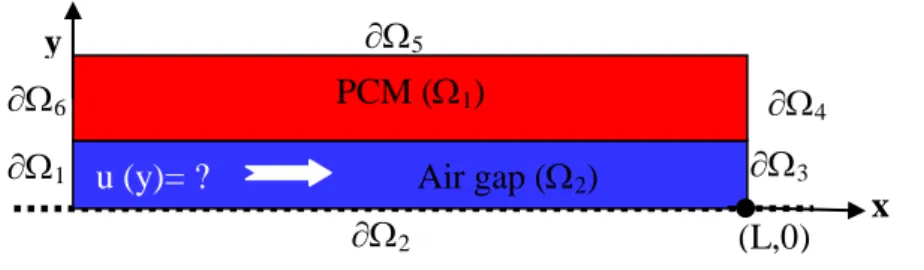
For the symmetry reason, just a half of PCM and air gap was considered in the numerical model (Figure 3)

Figure 3 Considered domain and point (L,0) taken as location of experimental results

The PCM slab is composed of 6 ENERGAIN®, with thermophysical properties as summarized in Table 1 [24] Property Value Density 850 (kg/m3) 1 5 6

u (y)= ? Air gap (2)

2 3 PCM (1) ₄ (L,0) x y (a) (b)

Thermal conductivity 0.2 (W/m/K)*** Apparent heat capacity Cp(T) see Figure 4 Melting start temperature 13.6°C Freezing start temperature 23.5°C Melting peak temperature 22.2°C Freezing peak temperature 17.8°C

Table 1 Thermophysical properties of PCM slab

Figure 4 Apparent heat capacity of the PCM [41]

Concerning air (fluid domain), and due to temperature range work, we consider constant thermophysical properties reported at the reference temperature 20°C. Hence the flow is supposed incompressible.

For the velocity field, we suppose that the flow is a fully developed Poiseuil regime:





ksol=0.22 W/(m/K) and kliq=0.18 W/(m/K), because of small variation of k we work with average value 0.2

W/(m/K)

0

4

8

12

16

0

5

10

15

20

25

30

35

C

p

(k

J

/k

g

.K

)

T ( C)

where u is the mean velocity (the unknown parameter), and H is the height of the air gap. In

addition, because of the small height of the PCM sample, no free convection phenomenon in the liquid state of PCM is considered.

2.3 Direct Problem

The governing equations of conjugate heat transfer with respect to the assumptions considered in §2.2 are presented in the system below:

T k t T T cps s s 2 ) (      in(1) (2.3. 1) T k T y u c t T c_{pf f pf f} f 2 ) (       _  in (2) (2.3.2)

With initial conditions:

Tt=0=T0 (2.3.3)

And boundary conditions

0 . 

T n at i (i=2,6) (2.3.4) T=Tin at 1 (2.3.5)

A continuity heat flux is applied at the interface, as the velocity field vanishes at the fluid side.

2.4 Sensitivity Problem

In the considered work, we are looking for an unknown mean velocity; this must be deduced from temperature measurements taken at specified point from the calculus domain (the exit of heat exchanger).

The sensitivity problem is needed for the computation of the step size to correct the estimated unknown parameter. It is obtained by the differentiation of the system of equations (2.3. 1)-(2.3.5) with respect to the unknown parameter [42]

Let’s note

. The treatment of the system equations of the direct problem leads to the sensitivity problem (see Appendix A for calculation details)





And the gradient function of the problem is given by [43]:







Where the measured point is (L,0): the exit of the heat exchanger see Figure 3.

3 Numerical modeling and implementation in comsol software

Here, we used Matlab R2013a and Comsol software (5.0) based on finite element method to solve the systems of equations. The mesh consists of 11110 triangular elements and 1404 quadrilateral elements. The time step is automatically performed by the software. At each one, the system of equations (direct and sensitivity) was solved with the linear system solver

(PARDISO); with fully coupled option between heat conduction and convection transfers. Results have been stored every 15 min. Our model was run on a 2.7 GHz processor and a 4 Go RAMPC machine.

4 Computational procedure

The computational procedure for solving the inverse problem is summarized as follows: for a given u at iteration k.

Step 1: Integrate the direct problem (2.3. 1)-(2.3.5);

Step 2: Compute the index performance (2.1. 4), stop when the stopping criterion is reached

and keeps as desired mean velocity, if not go to step 3;

Step 3: Integrate the sensitivity system (2.4. 1)-(2.4. 5) and compute the gradient objective

function (2.4. 6)

Step 5: Update the velocity field u(k+1) and go back to step 1 until the specified stopping criterion is reached.

5 Results and Discussion

5.1 Validation of inverse problem model

In all simulations u= 0 m/s was taken as the initial value of the starting calculation. The error tolerance is fixed to 5×10-03 (from many tests, even when we increase the precision to 10-04, the final value of velocity or flow-rate was not different to this chosen value of tolerance. See Appendix B). 240m3/h 330m3/h Step It er u m/s Q(m 3 /h) _mean T°C max *_T° C It er u (m/s) Q(m 3 /h) _mean T°C max *_T° C Cooling 6 4.26 10-03 1.45 225 1.92 5.2 7 2.9 10 -03 2.14 332 0.96 4.67 Heating 8 1.41 10-03 1.41 220 1.07 3.11 11 10 -03 _{2.0 311 1.14 3.4} * _{Excluding the beginning of the process}

Table 2 Obtained results from applied inverse method

In Table 2 we summarize the main parameters for analyzing the performance of the method.

T denotes the absolute difference between experimental air temperature at the exit of the heat exchanger and the numerical one obtained by the flow rate with inverse method. Excluding the heating step (330m3/h), the method requires a small number of iterations to converge as clearly shown by Figure 5. In all the simulations, values close to the experimental one are obtained from the second iteration. For both flow rates, results show that the charging process involves higher flow rates than discharging (Qcharge>Qdisch). This is consistent with previous works [35-36].

Figure 5 Variation of mean velocity and error vs iteration:

(a) 240m3/h cooling, (b) 240m3/h heating, (c) 330m3/h cooling, (d) 330m3/h heating

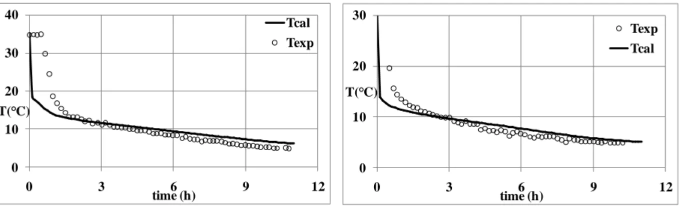
Figure 6 and Figure 7, show the comparison between experimental and simulated results for both flow rates in the charging and discharging step, respectively.

(a)

(d) (b)

Figure 6 cooling step : (left) 240m3/h; (right): 330 m3/h

Figure 7 heating step : (left) 240m3/h; (right): 330 m3/h

Regarding the quality aspect, the adopted method here, provides similar results to the experiments for the two processes. Plotted curves could be devised to three main stages:

For the quantity aspect, Table 2 shows the values of maximum and mean difference between experimental and numerical temperature. The main difference is observed at the beginning of the process, this is mainly due to the profile of the inlet temperature, which is time dependent in the experimental case, however it was kept constant in the model to simplify the development of the system of equation of the sensitivity problem (Figure 8).

So at the beginning of the charging process, the numerical temperature inlet is coldest than the experimental one, that’s why the model under estimate the exit temperature (Tcal<Texp). While

0 10 20 30 0 3 6 9 12 T( C) time (h) Texp Tcal 0 10 20 30 40 0 3 6 9 12 T( C) time (h) Tcal Texp 0 10 20 30 40 0 3 6 9 12 T( C) time (h) Texp Tcal 0 10 20 30 40 0 3 6 9 12 T( C) time (h) Texp Tcal

we observe the opposite phenomena in the discharging process (Tcal>Texp), as shown in figure 4 and 5. However as and when the two boundary conditions get closer we get a satisfactory results. Globally, the obtained results show that this simplification doesn’t have a big influence to the whole process.

Figure 8 Example of the inlet temperature profile used in experiments (ref [24]) and in the numerical model: Case of cooling (240m3/h)

On the other hand, concerning the difficulties to reach a precision less than 510-3, it is should be noted that resolving the sensitivity problem requires additional physical quantities (see

(2.4. 1)-(2.4. 2)): ( , , ); ( , , ); T(x,y,t) t t y x c t y x c_ps ps   

. For each iteration, these quantities are

stored at each time step during direct problem resolution, and injected later in the sensitivity system. In our case, we choose a 15 min as time step storing, because we considered this to be reasonable in relation to the time of the full process. This can, however induce some errors. We believe further works of parametric studies should be done in this area.

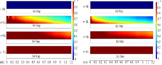
5.2 Charging process : Solid fraction

The main objective of the charging process is to achieve total freezing of the PCM sample. To analyze the performance of each flow rate we define the solid fraction parameter as:

T<Ts sf=1 s l l f l s T T T T s T T T      T>Tl sf=0 (5.2. 1) Where

Tl :the freezing starting temperature = 23.5°C [24]

Ts : the freezing peak temperature = 17.8°C [24]

Figure 9 Solid fraction in the PCM during charging process: (left) 1.15m/s, (right) 2.14m/s

Figure 9 shows that for the two obtained flow-rates, the fully freezing is obtained after 3 hours of the process. The freezing front moves progressively from left (inlet) to right. The small size of the PCM sample makes most likely makes the free convection phenomenon negligible. This may explain the uniformity of the treatment.

5.3 Discharging process : Liquid fraction

As for the charging process, we define the liquid fraction as : T>Tl’ lf=1 ' ' ' ' ' s l l f l s T T T T l T T T      T<T’s lf=0 (5.3. 1)

Where

Tl : freezing starting temperature = 22.2°C [24]

Ts : freezing peak temperature = 13.6°C [24]

Figure 10 Liquid fraction in the PCM during the discharging process: (left) 240m3/h, (right) 330 m3/h

For the discharging process similar observations are underlined concerning the uniformity of the treatment. Full fusion of the PCM requires more than 6 hours. This is mainly due to hysteresis phenomenon in the phase diagram of PCM (|Lfreezing|>|Lthawing|) see Figure 4.

It is well known that the free cooling exploits mainly latent heat of the PCM more than sensible heat. For the simulated cases, it is noted that the processing time largely exceeds the required time for the complete phase change, especially for the charging process.

All these elements show the advantage to extend the method to optimize the process with solid fraction as a set parameter of the target point for charging step, and respectively the liquid fraction for the discharging step.

6 Conclusion

An inverse method to estimate the air flow rate in a PCM exchanger was presented here. Because of the lack of studies in this area, the steps followed to obtain the final system of equations were widely detailed. “The conjugate gradient method with sensitivity problem” approach was adopted. The aforementioned method was applied to free cooling for 2 different flow-rate values in a discharging and charging process. Despite the complexity of the phenomena (non-linearity, conjugate heat transfer, coupled conduction and convection, phase change, hysteresis phenomenon…), the validation of numerical results shows the robustness and the consistency of this method. In the worst case, relative error does not exceed 510-03. As a preliminarily study, the obtained results remain satisfactory. However further parametric studies seem to be necessary to evaluate the impact of boundary conditions, time step for storing data, flow regime , etc. on the obtained results.

Our results reveal the importance of solid and liquid fractions to verify the full phase change and consequently the possibility to achieve the goal of the process. Hence it will be useful to use these parameters as constraint functions in an optimization control problem.

Appendix A: Formulation of Sensitivity problem

The Partial Differential Equations (PDE) of direct problem can be re-written as:

D(T)= 0 ) (  2    T k t T T cps s s  in(1) (A. 1) 0 2         T k T u c t T c_{pf f pf f} f   in (2) (A. 2)





If we derive the system (D) with respect to u and under conditions of regularity (to invert the

order of the derivatives), we obtain:

For (A. 1) :

 

and we obtain the final form of sensitivity problem of (A. 1):

0 ) ( ) ( ₂         s k t s T C s t T C s ps s ps s _  in Ω1 (A. 4)

The same way is applied to equation (A. 2), and we obtain

0 ) ( 2 3 2 2 2 2                 s k s y u T H y H t s Cpf f f  in(2) (A. 5)

The function to be minimized is given by:







And the gradient :







Appendix B: Results for tolerance error= 10-04 240m3/h 330m3/h Step It er U m/s Q(m 3_/h) mean T°C max T°C it er U(m/s) Q(m 3_/h) mean T°C max T°C Cooling 16 7.52 10-05 1.45 225 1.92 5.2 14 6.6 10-06 2.14 332 1 3 Heating 19 7.92 10-05 1.41 220 0.95 4.68 100 0.013 1.92 300 1.3 3.8

References

1 S. Kamali, “Review of free cooling system using phase change material for building”, Energy and Buildings.

(2014) 131-136.

2 L. Perez, J. Ortiz, J. Coronel, I. Maestre, A review of HVAC systems requirements in building energy regulations, Energy and Buildings. 43 (2011) 255–268.

3 A. Waqas, Z. U. Din, “Phase change material (PCM) storage for free cooling of buildings-A review”,

Renewable and Sustainable Energy Reviews. (2013) 608-625.

4 S. Takeda, K. Nagano, T. Mochida, and K. Shimakura, “Development of a ventilation system utilizing thermal energy storage for granules containing phase change material”, Solar Energy. 77(3) (2004) 329–338.

5 S. Alizadeh, M. Sadrameli, “Development of free cooling based ventilation technology for buildings: Thermal energy storage (TES) unit, performance enhancement techniques and design considerations – A review”, Renewable and Sustainable Energy Reviews. 58 (2016) 619-645.

6 G. Hed, R. Bellander, “Mathematical modelling of air heat exchanger”, Energy and Buildings. 38 (2006) 82–

89.

7 B. Zalba, J. M. Mar _{n, L. F. Cabeza, H. Mehling, “Review on thermal energy storage with phase change:} materials, heat transfer analysis and applications”, Applied Thermal Engineering. 23(3) (2003) 251-283.

8 A. Felix Regin, S.C. Solanki, J.S. Saini, “Heat transfer characteristics of thermal energy storage system using

PCM capsules: A review”, Renewable and Sustainable Energy Reviews. 12(9) (2008) 2438-2458.

9 V. V. Tyagi, D. Buddhi, “PCM thermal storage in buildings: A state of art, Renewable and Sustainable”, Energy Reviews. 11(6) (2007) 1146-1166.

10 A. Sharma, V.V. Tyagi, C.R. Chen, D. Buddhi, “Review on thermal energy storage with phase change

materials and applications”, Renewable and Sustainable Energy Reviews. 13(2) (2009) 318-345.

11 Y. Sun, J. Pei, Y. Cui, J. X, J. Liu, S. Pan, The 9th International Symposium on Heating, Ventilation and Air Conditioning (ISHVAC) joint with the 3rd International Conference on Building Energy and Environment

(COBEE), 12-15 July 2015, Tianjin, China Review of Phase Change Materials Integrated in Building Walls for Energy Saving, Procedia Engineering, Volume 121, 2015, Pages 763-770.

12 M. Iten, S. Liu, A. Shukla, “A review on the air-PCM-TES application for free cooling and heating in the

buildings”, Renewable and Sustainable Energy Reviews. 61 (2016) 175-186.

13 A. Sharifi, Y. Yamagata, “Roof ponds as passive heating and cooling systems: A systematic review”, Applied

Energy. 160 (2015) 336-357.

14 M. Medrano, M.O. Yilmaz, M. Nogués, I. Martorell, Joan Roca, Luisa F. Cabeza, “Experimental evaluation of commercial heat exchangers for use as PCM thermal storage systems”, Applied Energy. 86(10) (2009) 2047-2055.

15 A. Reyes, D. Negrete, A Mahn, F Sepúlveda, “Design and evaluation of a heat exchanger that uses paraffin wax and recycled materials as solar energy accumulator”, Energy Conversion and Management.88 (2014) 391-398.

16 T.Nomura, M. Tsubota, N. Okinaka, T. Akiyama."Improvement on Heat Release Performance of Direct-contact Heat Exchanger Using Phase Change Material for Recovery of Low Temperature Exhaust Heat", ISIJ International. 55(2) (2015) 441-447.

17 M. Labat, J. Virgone, D. David, F. Kuznik, “Experimental assessment of a PCM to air heat exchanger storage system for building ventilation application”, Applied Thermal Engineering. 66(1–2) (2014) 375-382.

18 M.Jaworski, “Thermal performance of building element containing phase change material (PCM) integrated with ventilation system – An experimental study”, Applied Thermal Engineering. 70(1, 5) (2014) 665-674.

19 S. N. Al-Saadi, Z.J.Zhai, “Systematic evaluation of mathematical methods and numerical schemes for modeling PCM-enhanced building enclosure”, Energy and Buildings. 92 (2015) 374-388.

20 P. Tittelein, S. Gibout, E. Franquet, K. Johannes, L. Zalewski, F. Kuznik, J. P. Dumas, S. Lassue, J. P. Bédécarrats, D. David, “Simulation of the thermal and energy behaviour of a composite material containing encapsulated-PCM: Influence of the thermodynamical modeling”, Applied Energy. 140(15) (2015) 269-274.

21 A. Ousegui, A. Le Bail, M. Havet, “Numerical and experimental study of a natural convection thawing process”, AIChE J, 52 (2006) 4240–4247.

22 V. Dubovsky, G. Ziskind, R. Letan, “Analytical model of a PCM-air heat exchanger”, Applied Thermal Engineering. 31(16) (2011) 3453-3462.

23 M. Bottarelli, M. Bortoloni, Y. Su, C. Yousif, A. A. Ayd n, A. Georgiev, “Numerical analysis of a novel ground heat exchanger coupled with phase change materials”, Applied Thermal Engineering. 88(5) (2015) 369-375.

24 J. P. A. Lopez, F. Kuznik, D, Baillis, J, Virgone, “Numerical modeling and experimental validation of a PCM to air heat exchanger”, Energy and Buildings. 64 (2013) 415-422.

25 V. A. A. Raj, R. Velraj, “Heat transfer and pressure drop studies on a PCM-heat exchanger module for free cooling applications”, International Journal of Thermal Sciences. 50(8) (2011) 1573-1582.

26 A. A. Al-Abidi, S. Mat, K. Sopian, M. Y. Sulaiman, T. M. Abdulrahman, “Numerical study of PCM solidification in a triplex tube heat exchanger with internal and external fins”, International Journal of Heat and Mass Transfer. 61 (2013) 684-695.

27 M. Jaworski, P. Łapka, P. Furmański, “Numerical modelling and experimental studies of thermal behaviour of building integrated thermal energy storage unit in a form of a ceiling panel”, Applied Energy. 113 (2014) 548-557.

28 A. Reyes, L. Henríquez-Vargas, R. Aravena, F. Sepúlveda, “Experimental analysis, modeling and simulation of a solar energy accumulator with paraffin wax as PCM”, Energy Conversion and Management. 105 (2015) 189-196.

29 J. Borderon, J. Virgone, R. Cantin, “Modeling and simulation of a phase change material system for improving summer comfort in domestic residence”, Applied Energy. 140 (2015) 288-296.

30 C. Arkar, S. Medved, “Free cooling of a building using PCM heat storage integrated into the ventilation system”, Solar Energy. 81(9) (2007) 1078-1087.

31 A. de Gracia, L. Navarro, A. Castell, L. F. Cabeza, “Numerical study on the thermal performance of a ventilated facade with PCM”, Applied Thermal Engineering. 61(2, 3) (2013) 372-380.

32 B.L. Gowreesunker, S.A. Tassou, M. Kolokotroni, “Coupled TRNSYS-CFD simulations evaluating the performance of PCM plate heat exchangers in an airport terminal building displacement conditioning system”, Building and Environment. 65 (2013) 132-145.

33 M. Thambidurai, K. Panchabikesan, K. N. Mohan, V. Ramalingam, “Review on phase change material based

free cooling of buildings-The way toward sustainability”, Journal of Energy Storage. 4 (2015) 74-88.

34 C. Arkar, S. Medved, “Free cooling of a building using PCM heat storage integrated into the ventilation

system", Solar Energy. 81(10) (2007) 78–87.

35 C. Arkar, B. Vidrih, S. Medved, “Efficiency of free cooling using latent heat storage integrated into the

36 B. Zalba, J. Marin, L. Cabeza, H. Mehling, “Free-cooling of buildings with phase change materials”,

International Journal of Refrigeration. 27 (2004) 39–49.

37 W. Saman, F. Bruno, E. Halawa. “Thermal performance of PCM thermal storage unit for a roof integrated

solar heating system”. Solar Energy. 78 (2005) 341–349.

38 A. Waqas, S. Kumar, “Thermal performance of latent heat storage for free cooling of buildings in a dry and

hot climate: an experimental study”, Energy Build. 43 (2011) 2621–2630.

39 Xiuzhang Fu, Dingxin Wu, Comparison of the Efficiency of Building Hybrid Ventilation Systems with Different Thermal Comfort Models, Energy Procedia, Volume 78, 2015, Pages 2820-2825

40 H. Molavi, R. K. Rahmani, A. Pourshaghaghy, E. S. Tashnizi, A. H. Fard, “Heat Flux Estimation in a Nonlinear Inverse Heat Conduction Problem With Moving Boundary”, Journal of Heat Transfer. 132(8) (2010)

41 J. Borderon, “Intégration des matériaux à changement de phase comme système de régulation dynamique en rénovation thermique” [PhD thesis]. ENTPE: Lyon; (2012)

42 Wagner M. Brasil, Jian Su, Atila P. Silva Freire, An inverse problem for the estimation of upstream velocity profiles in an incompressible turbulent boundary layer, International Journal of Heat and Mass Transfer, Volume 47, Issue 6, 2004, Pages 1267-1274

43 Thermal Measurements and Inverse Techniques. Edited by Renato M . Cotta. CRC Press 2011. Print ISBN: 978-1-4398-4555-4