Probabilistic Analysis and Design of Circular Tunnels against Face Stability

(1)

HAL Id: hal-00907009

https://hal.archives-ouvertes.fr/hal-00907009

Submitted on 20 Nov 2013

HAL is a multi-disciplinary open access

archive for the deposit and dissemination of

sci-entific research documents, whether they are

pub-lished or not. The documents may come from

teaching and research institutions in France or

abroad, or from public or private research centers.

L’archive ouverte pluridisciplinaire HAL, est

destinée au dépôt et à la diffusion de documents

scientifiques de niveau recherche, publiés ou non,

émanant des établissements d’enseignement et de

recherche français ou étrangers, des laboratoires

publics ou privés.

Probabilistic Analysis and Design of Circular Tunnels

against Face Stability

Guilhem Mollon, Dias Daniel, Soubra Abdul-Hamid

To cite this version:

Guilhem Mollon, Dias Daniel, Soubra Abdul-Hamid. Probabilistic Analysis and Design of Circular

Tunnels against Face Stability. International Journal of Geomechanics, American Society of Civil

Engineers, 2009, 9 (6), pp.237-249. �10.1061/ASCE1532-364120099:6237�. �hal-00907009�

(2)

Probabilistic Analysis and Design of Circular Tunnels

against Face Stability

Guilhem Mollon

1

; Daniel Dias

2

; and Abdul-Hamid Soubra, M.ASCE

3

Abstract: This paper presents a reliability-based approach for the three-dimensional analysis and design of the face stability of a shallow circular tunnel driven by a pressurized shield. Both the collapse and the blow-out failure modes of the ultimate limit state are studied. The deterministic models are based on the upper-bound method of the limit analysis theory. The collapse failure mode was found to give the most critical deterministic results against face stability and was adopted for the probabilistic analysis and design. The random variables used are the soil shear strength parameters. The Hasofer-Lind reliability index and the failure probability were determined. A sensitivity analysis was also performed. It was shown that 共1兲 the assumption of negative correlation between the soil shear strength parameters gives a greater reliability of the tunnel face stability with respect to the one of uncorrelated variables; 共2兲 FORM approximation gives accurate results of the failure probability; and 共3兲 the failure probability is much more influenced by the coefficient of variation of the angle of internal friction than that of the cohesion. Finally, a reliability-based design is performed to determine the required tunnel pressure for a target collapse failure probability.

DOI: 10.1061/共ASCE兲1532-3641共2009兲9:6共237兲

CE Database subject headings: Tunnels; Pressure; Passive pressure; Limit analysis; Probability; Design.

Introduction

Over the past 30 years, tunneling in a frictional and/or cohesive soil has been possible due to recent technological advances in-cluding the pressurized shield. Face stability analysis of shallow circular tunnels driven by the pressurized shield is of major im-portance. The tunnel face pressure must avoid both the collapse 共active failure兲 and the blow-out 共passive failure兲 of the soil mass nearby the tunnel face. Active failure of the tunnel is triggered by application of surcharge and self-weight, with the tunnel face pressure providing resistance against collapse. Under passive con-ditions, these roles are reversed and the face pressure causes blow-out with resistance being provided by the surcharge and self-weight.

In this paper, the face stability analysis is conducted based on a probabilistic approach. The reliability-based analysis is more rational than the deterministic one since it takes into account the inherent uncertainty of the input variables. Nowadays, this is pos-sible because of the improvement of our knowledge on the statis-tical properties of the soil 共Phoon and Kulhawy 1999; Baecher and Christian 2003兲. Two performance functions may characterize

the tunnel behavior: the serviceability limit state and the ultimate limit state 共ULS兲. Only the collapse and the blow-out failure modes of the ULS are analyzed herein. Two new rigorous deter-ministic limit analysis models are used. The soil shear strength parameters are modeled as random variables. The main reliability concepts are described next, followed by the two deterministic models and discussions of the deterministic and probabilistic nu-merical results based on these models.

Overview of Reliability Concepts

The reliability index is a measure of the safety that takes into account the inherent uncertainties of the input variables. A widely used reliability index is the Hasofer and Lind 共1974兲 index. Its matrix formulation is 共Ditlevsen 1981兲

␤HL= min

x苸F

冑

共x − ␮兲T_C−1_{共x − ␮兲} _共1兲 in which x = vector representing the n random variables; ␮ = vector of their mean values; C = covariance matrix; and F = failure region. The minimization of Eq. 共1兲 is performed subject to the constraint G共x兲艋0 where the limit state surface G共x兲=0, separates the n dimensional domain of random variables into two regions: a failure region F represented by G共x兲艋0 and a safe region given by G共x兲⬎0.

The classical approach for computing ␤HLby Eq. 共1兲 is based on the transformation of the limit state surface into the rotated space of standard normal uncorrelated variates. The shortest dis-tance from the transformed failure surface to the origin of the reduced variates is the reliability index ␤HL.

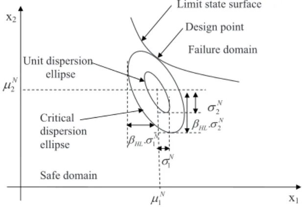
An intuitive interpretation of the reliability index was sug-gested in Low and Tang 共1997a, 2004兲 where the concept of an expanding ellipsoid 关or an ellipse in two-dimensions 共2D兲 as shown in Fig. 1兴 led to a simple method of computing the Hasofer-Lind reliability index in the original space of the random 1

Ph.D. Student, INSA Lyon, LGCIE Site Coulomb 3, Géotechnique, Bât. J.C.A. Coulomb, Domaine scientifique de la Doua, 69621 Villeur-banne cedex, France. E-mail: Guilhem.Mollon@insa-lyon.fr

2

Associate Professor, INSA Lyon, LGCIE Site Coulomb 3, Géotech-nique, Bât. J.C.A. Coulomb, Domaine scientifique de la Doua, 69621 Villeurbanne cedex, France. Email: Daniel.Dias@insa-lyon.fr

3

Professor, Dept. of Civil Engineering, Univ. of Nantes, Bd. de l’université, BP 152, 44603 Saint-Nazaire, France 共corresponding author兲. E-mail: Abed.Soubra@univ-nantes.fr

Note. This manuscript was submitted on April 25, 2008; approved on July 1, 2009; published online on November 13, 2009. Discussion period open until May 1, 2010; separate discussions must be submitted for indi-vidual papers. This paper is part of the International Journal of

Geome-chanics, Vol. 9, No. 6, December 1, 2009. ©ASCE, ISSN 1532-3641/ 2009/6-237–249/$25.00.

(3)

variables using an optimization tool available in most software packages. Low and Tang 共1997a,2004兲 reported that the Hasofer-Lind reliability index ␤HLmay be regarded as the codirectional axis ratio of the smallest ellipsoid that just touches the limit state surface to the unit dispersion ellipsoid 关i.e., corresponding to ␤HL= 1 in Eq. 共1兲 without the minimum兴. They also stated that finding the smallest ellipsoid 共called hereafter critical ellipsoid兲 that is tangent to the limit state surface is equivalent to finding the most probable failure point. When the random variables are non-normal, the Rackwitz-Fiessler equivalent normal transformation was used to compute the equivalent normal mean ␮N _{and the}

equivalent normal standard deviation ␴N_{. The iterative}

computa-tions of ␮N_{and ␴}N_{for each trial design point are automatic during}

the constrained optimization search.

From the first-order reliability method FORM and the Hasofer-Lind reliability index ␤HL, one can approximate the failure prob-ability as follows:

Pf⬇ ⌽共− ␤HL兲共2兲

where ⌽共·兲=cumulative distribution function of a standard nor-mal variable. In this method, the limit state function is approxi-mated by a hyperplane tangent to the limit state surface at the design point.

Monte Carlo 共MC兲 is another method of computing the failure probability. It is the most robust simulation method in which samples are generated with respect to the probability density of each variable. For each sample, the response of the system is calculated. An unbiased estimator of the failure probability is given by P ˜ f= 1 N

兺

i=1 N I共xi兲共3兲

where N = number of samples and I共x兲=1 if G共x兲艋0 and 0 else-where. The coefficient of variation of the estimator is given by

COV共P˜

f兲 =

冑

共1 − Pf兲

PfN

共4兲 Generally, for a given target of the coefficient of variation, the crude MC simulation requires a large number of samples, i.e., a large computation time. This is especially the case for small values of the failure probability. The importance sampling 共IS兲 simulation method is a more efficient approach; it requires fewer sample points than the MC method. In this approach, the initial sampling density f共·兲 is shifted to the design point in order to

concentrate the samples in the region of greatest probability den-sity within the zone defined by G共x兲艋0. The design point may be determined by using any of the classical methods such as Rackwitz-Fiessler algorithm 共Rackwitz and Fiessler 1978兲, Low and Tang’s ellipsoid approach 共Low and Tang 1997a, 2004兲, etc. An estimator of the failure probability Pf is obtained as follows

共Melchers 1999兲: P ˜ f= 1 N

兺

_i₌₁ N I共v_i兲f共 v_i兲 h共v_i兲共5兲 where h共·兲=new sampling density centered at the design point andv= vector of sample values generated with the new

probabil-ity densprobabil-ity function 共PDF兲, i.e., h共·兲. The coefficient of variation of the estimator is given by 共Melchers 1999兲

COV共P˜ f兲 = 1 Pf

冑

1 N

冉

1 N

兺

_i=1 N

冉

I共v_i兲f共 v_i兲 h共v_i兲

冊

2 −共P_f兲2

冊

_共6兲

Reliability Analysis of a Circular Tunnel Face

The aim of this paper is to perform a reliability analysis of the face stability of a shallow circular tunnel driven by a pressurized shield in a c-␸ soil. The problem can be idealized as shown in Figs. 2共a and b兲 by considering a circular rigid tunnel of diameter D driven under a depth of cover C. A surcharge ␴_sis applied at the ground surface and a uniform retaining pressure ␴tis applied

to the tunnel face to simulate tunneling under compressed air. The deterministic models are based on the upper-bound method of the limit analysis theory. They are presented in the next sec-tion. Due to uncertainties in soil shear strength parameters, the cohesion c, and the angle of internal friction ␸ are considered as random. They are modeled in the present analysis as random vari-ables. This means that the soil parameters are considered as ho-mogeneous in the whole soil mass. The randomness of the soil is taken into account from one simulation to another. The perfor-mance functions G₁ and G₂ used in the reliability analysis for both the collapse and the blow-out cases are respectively defined as follows:

G1= ␴t− ␴c 共7兲

G2= ␴b− ␴t 共8兲

where ␴_t= applied pressure on the tunnel face, and ␴_c and ␴b=collapse and blow-out pressures, respectively.

Limit Analysis Models

Several theoretical models have been presented in literature for the computation of the collapse and blow-out tunnel pressures corresponding respectively to the active and passive modes of failure. The most recent and significant approach is the one pre-sented by Leca and Dormieux 共1990兲 who considered three-dimensional 共3D兲 failure mechanisms in the framework of the upper-bound method in limit analysis. In this paper, two new deterministic models 共3D multiblock failure mechanisms兲 based on the upper-bound approach of limit analysis are proposed for the probabilistic analysis. These mechanisms constitute an im-provement of the failure mechanisms by Leca and Dormieux 共1990兲 since they allow the 3D slip surface to develop more freely in comparison with the available one- and two-block mechanisms Failure domain

Safe domain

Limit state surface

Design point Critical dispersion ellipse N HL.σ2 β N 2 σ N 1 σ Unit dispersion ellipse N 1 μ N 2 μ x1 x2 N HL.σ1 β

Fig. 1. Design point and equivalent normal dispersion ellipses in the

space of two random variables

(4)

given by Leca and Dormieux 共1990兲. Notice that the use of a lower-bound approach in limit analysis 共using for instance finite elements and linear programming兲 is another alternative ap-proach. It has the advantage of providing conservative solutions. However, this method leads, when dealing with the probabilistic analysis, to complex and very expensive numerical computations with a high computation time since the probabilistic analysis re-quires a significant number of calls of the deterministic model for a given soil variability. Thus, in order to optimize the computation time and to get sufficiently accurate results, efforts were concen-trated in the present paper on the improvement of the best avail-able upper-bound solutions 共i.e., those by Leca and Dormieux 1990兲 by using multiblock failure mechanisms. Notice that a multiblock failure mechanism was also used by Soubra 共1999兲 when dealing with the 2D analysis of the bearing capacity of strip foundations. It was shown by Soubra 共1999兲 that the multiblock mechanism significantly improves the solutions of the bearing capacity as given by the available mechanisms 共two-block and log-sandwich mechanisms兲 and obtains smaller 共i.e., better兲 upper bounds. This is due to the great freedom offered by this mecha-nism to move more freely with respect to traditional mechamecha-nisms.

The optimal radial shear zone found in the case of a ponderable soil was not bounded by a log spiral as is the case of the tradi-tional Prandtl 共i.e., log sandwich兲 mechanism but by a more criti-cal surface found by numericriti-cal optimization. Furthermore, the multiblock mechanism by Soubra 共1999兲 led in some cases 共for Nqand Nc兲 to the exact solutions given by the log-sandwich

fail-ure mechanism since both upper and lower bound solutions were identical in these cases. Notice finally that the two 3D multiblock failure mechanisms presented in this paper for the stability analy-sis of circular tunnels make use of the idea of multiblock mecha-nisms suggested by Soubra 共1999兲 in the 2D analysis of strip footings in order to obtain better upper-bound solutions. A de-tailed description of these mechanisms is given in the following sections.

Collapse Mechanism M1 (Active Case)

M1 is an improvement of the two-block collapse mechanism pre-sented by Leca and Dormieux 共1990兲. This mechanism is a multi-block. It is composed of n truncated rigid cones with circular cross sections and with opening angles equal to 2␸. Fig. 2共c兲 depicts three different 3D views of a five-block mechanism 共i.e., n= 5兲. The geometrical construction of this mechanism is similar to that of Leca and Dormieux 共1990兲, i.e., each cone is the mirror image of the adjacent cone with respect to the plane that is normal to the contact surface separating these cones 共cf. Leca and Dormieux 1990兲. This is a necessary condition to assure the same elliptical contact area between adjacent cones. In order to make clearer the geometrical construction of the 3D failure mechanism, Fig. 3 shows how the first two truncated conical blocks adjacent to the tunnel face are constructed. The geometrical construction of the remaining truncated conical blocks is straightforward. In Fig. 3, Block 1 is a truncated circular cone adjacent to the tunnel face. It has an opening angle equal to 2␸ 共in order to respect the normality condition in limit analysis兲 and an axis inclined at ␣ with the horizontal direction. Thus, the intersection of this trun-cated cone with the tunnel face is an elliptical surface that does not cover the entire circular face of the tunnel 关cf. Fig. 2共c兲兴 This is a shortcoming not only of the present failure mechanism but also of the one- and two-block mechanisms by Leca and Dormieux 共1990兲. On the other hand, Block 1 is truncated with Plane 1, which is inclined at an angle ␤1with the vertical direc-tion 共cf. Fig. 3兲. In order to obtain the same contact area with the adjacent truncated conical block, Block 2 is constructed in such a manner to be the mirror image of Block 1 with respect to the plane that is normal to the surface separating the two blocks 共i.e., Plane 2 as shown in Fig. 3兲. The upper rigid cone will or will not intersect the ground surface depending on the ␸ and C / D values. At first glance, the fact that the failure mechanism does not intersect the ground surface for some values of ␸ and C / D is striking. However, the same phenomenon was also observed

c. Three-dimensional views of the M1 mechanism in the (x, y, z) space a. M1 mechanism (collapse case) in the (y, z) plane

b. M2 mechanism (blow-out case) in the (y, z) plane

Fig. 2. Failure mechanisms M1 and M2 for the face stability

Fig. 3. Detail of the construction of the M1 mechanism in the共y ,z兲 plane

(5)

when performing 3D numerical simulations using FLAC3D soft-ware 共Mollon et al. 2009兲. Notice that while using numerical simulations, no assumptions were made on the shape of the fail-ure mechanism and the optimal failfail-ure mechanism was explored. Thus, one may confirm that the present failure mechanism based on limit analysis is acceptable even if the critical failure surface does not outcrop.

M1 is a translational kinematically admissible failure mecha-nism. The different truncated conical blocks of this mechanism move as rigid bodies. These truncated rigid cones translate with velocities of different directions, which are collinear with the cones axes and make an angle ␸ with the conical discontinuity surface in order to respect the normality condition required by the limit analysis theory. The velocity of each cone is determined by the condition that the relative velocity between the cones in con-tact has the direction that makes an angle ␸ with the concon-tact surface. The velocity hodograph is presented in Fig. 2共a兲. The present mechanism is completely defined by n angular parameters ␣and ␤i共i=1, ... ,n−1兲 where n is the number of the truncated

conical blocks.

Blow-Out Mechanism M2 (Passive Case)

Even though safety against collapse is a major concern during tunneling, the blow-out mechanism may be of interest for very shallow tunnels bored in weak soils, when the pressure ␴t

can become so great that soil is heaved in front of the shield. M2 关Fig. 2共b兲兴 is a blow-out mechanism. It represents the passive case of the former mechanism. With reference to M1, the M2 mecha-nism presents an upward movement of the soil mass. Thus, the cones with an opening angle 2␸ are reversed. Contrary to M1, the present mechanism always outcrops.

Ellipsoid Approach via Spreadsheet

In the present paper, by the Low and Tang 共1997a, 2004兲 method, one literally sets up a tilted ellipsoid in the Excel spreadsheet and minimizes the dispersion ellipsoid subject to the constraint that it be tangent to the limit state surface using the Excel Solver with the automatic scaling option. Eq. 共1兲 may be rewritten as 共Low and Tang 1997b, 2004; Youssef Abdel Massih and Soubra 2008; Youssef Abdel Massih et al. 2008兲

␤HL= min x苸F

冑冋

x− ␮N ␴N

册

T 关R兴−1

冋

x− ␮ N ␴N

册

共9兲

in which 关R兴−1_{⫽inverse of the correlation matrix. This equation} will be used 关instead of Eq. 共1兲兴 since the correlation matrix关R兴 displays the correlation structure more explicitly than the covari-ance matrix关C兴.

Deterministic Numerical Results

For both M1 and M2 mechanisms, when the total rate of energy dissipation and the total rate of external work are equated, the ultimate tunnel pressure ␴u for the collapse and the blow-out

modes of failure can be expressed as follows:

␴_u= ␥DN_␥+ cN_c+ ␴_sNs 共10兲

where N␥, Nc, and Ns= nondimensional coefficients. They

repre-sent, respectively, the effect of soil weight, cohesion, and sur-charge loading. The expressions of the different coefficients N_␥, Nc, and Ns are given in the Appendix. Notice that the external

forces involved in the present mechanisms are the weights of the different truncated rigid cones, the surcharge loading acting on the ground surface, and the pressure applied on the tunnel face. For the collapse mechanism, the rate of external work of the surcharge loading should be calculated only in case of outcrop of the mechanism on the ground surface. The computation of the rate of external work of the different external forces is straight-forward. The details are given in Oberlé 共1996兲. The rate of in-ternal energy dissipation takes place along the different velocity discontinuity surfaces. These are 共1兲 the radial elliptical surfaces which are the contact areas between adjacent truncated cones and 共2兲 the lateral surfaces of the different truncated cones. Notice that the rate of internal energy dissipation along a unit velocity discontinuity surface is equal to c · ␦u 共Chen 2008兲 where c is the soil cohesion and ␦u is the tangential component of the velocity along the velocity discontinuity surface. Calculations of the rate of internal energy dissipation along the different velocity discon-tinuity surfaces are straightforward. The details are given in Oberlé 共1996兲.

In Eq. 共10兲, ␴_u, N_␥, N_c, and N_s depend not only on the mechanical and geometrical characteristics c, ␸, and C / D, but also on the angular parameters of the failure mechanism ␣ and ␤i

共i=1, ... ,n−1兲. In the following sections, the ultimate tunnel pressure of the collapse mode will be denoted ␴_c, and that of blow-out will be refereed to as ␴_b. They were obtained respec-tively by maximization and minimization of ␴_uin Eq. 共10兲 with respect to the ␣ and ␤iangles. As for the ultimate tunnel

pres-sures, the critical coefficients N_␥b_{, N} c b_{, and N} s b_{共respectively N} ␥ c_{, N} c c_,

and N_sc_{兲 corresponding to the blow-out 共respectively collapse兲}

case, were obtained by minimization 共respectively maximization兲 of these coefficients with respect to the ␣ and ␤iangles. A

com-puter program has been written in Microsoft Excel Visual Basic to define the different coefficients N␥, Nc, and Ns and the tunnel

pressure ␴_u for the collapse and the blow-out modes of failure. The optimization was performed using the optimization tool “Solver” implemented in Microsoft Excel. It was shown that the increase in the number of cones improves the solutions 共i.e., in-creases the active coefficients, and reduces the passive ones兲. The numerical results have shown that this improvement becomes in-significant 共smaller than 1%兲 for a number of blocks greater than five. Therefore, only five blocks were used in this paper for the collapse and the blow-out mechanisms.

Notice that in both the collapse and the blow-out cases, the numerical results have shown that N_c and N_s are related by the following classical formula:

Nctan ␸ + 1 − Ns= 0 共11兲

This can be explained by the theorem of corresponding states 共Soubra 1999兲. Hence, in the following, only the N␥and Ns

coef-ficients will be presented; the N_ccoefficient can be obtained using Eq. 共11兲.

Comparison with Available Upper-Bound Solutions

Leca and Dormieux 共1990兲 have considered a collapse failure mechanism composed of two rigid cones. Fig. 4 presents the N_␥c

and N_scvalues given by the present analysis 共M1 mechanism兲 and the ones given by Leca and Dormieux 共1990兲. The N_␥c coefficient increases with C / D; then, it becomes constant for large values of C / D corresponding to the condition of no outcrop of the upper block. However, coefficient N_sc _{decreases with the C / D increase}

and vanishes beyond a certain value of C / D corresponding to the no-outcrop condition. In this case, the surcharge loading has no

(6)

influence on the critical N_sc _{value. These conclusions conform}

to those of Leca and Dormieux 共1990兲. It should be mentioned that in the case of collapse, the present failure mechanism gives greater upper-bound solutions than the available upper-bound solutions proposed by Leca and Dormieux 共1990兲. The improve-ment of the solution is about 8% for the N_␥c _{coefficient when}

␸= 20° and C / D ⬎ 0.55. For N_sc_{, the improvement is equal to}

37.5% when ␸ = 20° and C / D = 0.1.

For the blow-out case, Leca and Dormieux 共1990兲 have con-sidered a mechanism composed of a single rigid cone moving upward. The upper-bound solutions given by these writers are compared with the ones corresponding to the present M2 mecha-nism in Fig. 5. The M2 mechamecha-nism is better than the one pre-sented by Leca and Dormieux 共1990兲 since the present upper-bound solutions are smaller. For the N_␥b _{coefficient, the reduction}

is very significant and it is of 41% when ␸ = 30° and C / D = 1.4. For the N_sb coefficient, significant reductions are also obtained with respect to the results presented by Leca and Dormieux. For example, when ␸ = 30° and C / D = 1.4, the reduction attains 51%. As a conclusion, the four design charts presented before 共i.e., Figs. 4 and 5兲 give the values of the coefficients N␥and Nsof the

proposed mechanisms for both the collapse and blow-out cases for different values of the governing parameters ␸ and C / D. The existing values by Leca-Dormieux are also given in these charts, allowing one to appreciate the improvement with respect to prior solutions. The determination of the critical collapse or blow-out pressure to be used in practice can then be made by using Eq. 共10兲 where N_cin this equation is given by Eq. 共11兲 and N_␥and N_sare given in the design charts of Figs. 4 and 5.

It should be mentioned here that Fig. 2共c兲 presented earlier is a 3D representation of the critical collapse mechanism obtained after optimization of the tunnel pressure with respect to the geo-metrical parameters of the failure mechanism for a friction angle

equal to 17° and a cohesion equal to 7 kPa when C / D = 2. It can be seen that the 3D critical failure mechanism M1 involves a radial shear zone 共composed of three small truncated rigid cones, i.e., Blocks 2–4兲 sandwiched between two greater rigid cones 共i.e., Blocks 1 and 5兲. Line BCDE as obtained by numerical op-timization is not a log spiral and this constitutes the major interest of the present multiblock mechanism with respect to the similar in shape mechanism 共i.e., log sandwich兲 where line BCDE is re-placed by a log spiral.

For the currently encountered cases 共i.e., 1 艋 C / D 艋 3; 10° 艋 ␸ 艋30°; 0 艋 c 艋 20 kPa兲, Table 1 presents the results of the tunnel ultimate pressures ␴cand ␴bcorresponding respectively to

the collapse and the blow-out modes of failure as given by the present failure mechanisms. The applied tunnel pressure ␴_tshould be greater than the collapse pressure ␴_cto avoid the active failure. If one adopts a safety factor against collapse共Fs= ␴t/␴c兲 equal to

2, the required applied pressure ␴_tshould be equal to twice the value of the collapse pressure as given in the fifth column of Table 1. The comparison of these pressures with those of the blow-out case 共i.e., ␴b兲 shows that the blow-out pressures are

much higher than the practical applied tunnel pressures ␴_tfor all the values of the governing parameters considered in this paper. Hence, the blow-out mode of failure does not occur for the cases currently encountered in practice. In the following sections, only the collapse failure mode is considered in the probabilistic analy-sis and design of circular tunnels against face stability.

Comparison with Three-Dimensional Numerical Simulations

In order to assess the accuracy of the limit analysis collapse model, complex 3D numerical simulations were performed using

Fig. 4. N_␥c _{and N} s

c _{versus C/D as given by Leca and Dormieux and}

M1 mechanism Fig. 5. N_␥b _{and N}

s

b_{versus C/D as given by Leca and Dormieux and}

M2 mechanism

(7)

the finite difference commercial software FLAC3D_{. They allow} one to determine the values of the critical collapse pressure ␴_c. For a detailed description of these simulations, the reader may refer to Mollon et al. 共2009兲 . Fig. 6共a兲 shows a comparison be-tween the collapse pressures as given by the FLAC3D_{model and} by the M1 mechanism. Three cases of 共c,␸兲 are considered to show the effect of both c and ␸ on the comparison between the limit analysis and the numerical simulations. It appears that the limit analysis results are not far from the ones obtained by FLAC3D_{. Even if they are upper-bounds 共i.e., nonconservative兲 to} the exact collapse pressures, the present collapse pressures given by limit analysis can be considered as sufficiently accurate for

practical use. Notice also that the very short calculation time re-quired by the limit analysis model 共smaller than 1 s兲 compared to that required by the numerical simulations 共90 min兲 is appealing for the probabilistic analysis, which requires a significant number of calls of the deterministic model for a given soil variability. Finally, Fig. 6共b兲 shows that the shape of the critical M1 collapse mechanism is very close to the one obtained by FLAC3D _{for the} reference case 共i.e., ␸ = 17°, c = 7 kPa兲 that will be studied in the probabilistic analysis.

Probabilistic Numerical Results

The present collapse failure mechanism M1 will be used in all subsequent probabilistic analyses since 共1兲 it gives better upper-bound solutions than the mechanism by Leca and Dormieux 共1990兲 and 共2兲 it gives results that are not very far from the solutions given by complex 3D numerical simulations using FLAC3D_.

The probabilistic numerical results presented in this paper con-sider the case of a circular tunnel with a diameter D = 10 m and a cover C = 10 m 共i.e., C / D = 1兲. The soil has a unit weight of 18 kN/ m3_{. No surcharge loading} _共␴

s= 0兲 is considered in the

analysis.

For the probability distribution of the random variables, two cases are studied. In the first case, referred to as normal variables, c and ␸ are considered as normal variables. In the second case, referred to as nonnormal variables, c is assumed to be lognor-mally distributed while ␸ is assumed to be bounded and a ␤ distribution is used 共Fenton and Griffiths 2003兲. The parameters of the ␤ distribution are determined from the mean value and standard deviation of ␸ 共Haldar and Mahadevan 2000兲. For both cases, correlated and uncorrelated variables are considered. In this paper, the illustrative values used for the statistical mo-ments of the shear strength parameters and their coefficient of correlation ␳c,␸are as follows: ␮c= 7 kPa, ␮␸= 17°, COVc= 20%,

COV␸= 10%, and ␳c,␸= −0.5.

A common approach to determine the reliability index of a stability problem 共slope stability, bearing capacity, etc.兲 is based on the calculation of the reliability index corresponding to the deterministic failure surface 共i.e., the one corresponding to the minimum safety factor or the ultimate load兲共Christian et al. 1994兲. In this paper, the reliability index is determined by mini-mizing the quadratic form of Eq. 共9兲 not only with respect to the random variables, but also with respect to the geometrical param-eters of the failure mechanism 共␣,␤i兲 i=1,..,n−1 共Bhattacharya

et al. 2003; Youssef Abdel Massih 2007; Youssef Abdel Massih et al. 2008兲. Five rigid blocks 共i.e., n = 5 in Fig. 2兲 are considered.

Table 1. Values of the Collapse and Blow-Out Pressures ␴cand ␴band the Required Face Pressure ␴tfor a Safety Factor Fs= 2 for the Common Values

of C / D, ␸, and c C / D ␸ 共°兲 c 共kPa兲 ␴c 共kPa兲 ␴t共kPa兲 for Fs= 2 ␴b 共kPa兲 1 10 0 100 200 660

1 10 20 ⬍0 共i.e., stable兲 ⬍0 共i.e., stable兲 94

1 30 0 22 44 3,800

1 30 20 ⬍0 共i.e., stable兲 ⬍0 共i.e., stable兲 4,700

3 10 0 106 212 2,570

3 30 0 22 44 20,900

a. Critical collapse pressure

b. Failure pattern in the (y, z) plane

Fig. 6. Comparison between FLAC3D _{numerical simulations and} limit analysis

(8)

Therefore, the minimization is performed with respect to seven parameters 共␣,␤i, c , ␸兲. The surface obtained corresponding to

the minimum reliability index is referred to here as the critical probabilistic surface.

For the configuration presented earlier, the tunnel collapse pressure corresponding to normal variables was found equal to ␴c= 28.3 kPa. However, for nonnormal variables, the collapse

pressure was computed using the equivalent mean values of the random variables and was found equal to 28.8 kPa.

Reliability Index, Critical Dispersion Ellipses, and Partial Safety Factors

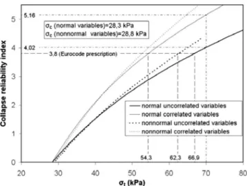
Fig. 7 presents the Hasofer-Lind reliability index versus the ap-plied pressure ␴tfor four combinations of normal and nonnormal,

uncorrelated and correlated shear strength parameters. For all cases, the reliability index increases with the increase of the tun-nel face pressure ␴_t. The comparison of the results of correlated variables with those of uncorrelated variables shows that the re-liability index corresponding to uncorrelated variables is smaller than the one of negatively correlated variables for both normal and nonnormal variables. One can conclude that assuming un-correlated shear strength parameters is conservative in compari-son to assuming negatively correlated parameters. For a target reliability index of 3.8 as imposed by Eurocode 7, the required tunnel pressure is smaller for correlated and nonnormal variables. For instance, with respect to the reference case of normal and uncorrelated variables, ␴t decreases by 19% if the variables are

correlated 共54.3 kPa to be compared to 66.9 kPa兲 and by 7% if the variables are considered to follow nonnormal distributions 共62.3 kPa to be compared to 66.9 kPa兲.

The values 共cⴱ_{and ␸}ⴱ_{兲 of the design points corresponding to} different values of the tunnel face pressure ␴_t can give an idea about the partial safety factors of each of the strength parameters cand tan ␸ as follows:

Fc= ␮c cⴱ 共12兲 F␸= tan共␮␸兲 tan ␸ⴱ 共13兲

Table 2 gives the obtained partial safety factors F_c and F␸ and

the corresponding design point and reliability index for the four combinations of normal, nonnormal, uncorrelated, and correlated variables and for different values of the tunnel face pressure ␴_t. This table also shows the empirical Fcand F␸ values suggested by Eurocode 7. For a reliability index close to 3.8 as suggested by Eurocode 7 in the ULS, the values obtained from the present approach for the four combinations of assumptions are between 1 and 1.5 for F_cand about 1.5 for F␸. The corresponding Eurocode values are 1.6 and 1.25. As can be seen, contrary to Eurocode 7, the present probabilistic approach attributes more safety to the cohesion parameter than Eurocode 7.

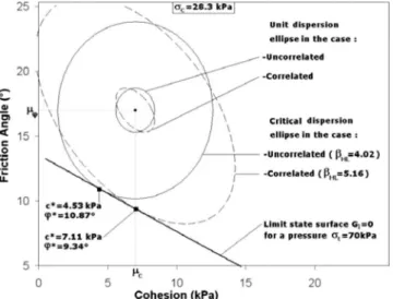
For ␴_t= 70 kPa 共Fig. 7兲, the collapse reliability index for un-correlated and un-correlated normal variables are respectively equal to 4.02 and 5.16. The corresponding most probable failure points obtained from the minimization procedure 共Table 2兲 are found to be at 共cⴱ_{= 4.53 kPa, ␸}ⴱ_{= 10.87°兲 and 共c}ⴱ_{= 7.11 kPa, ␸}ⴱ_{= 9.34°兲.} These are the points of tangency of the critical dispersion ellipses with the limit state surface. Notice that the limit state surface divides the combinations of共c,␸兲 that would lead to failure from the combinations that would not. The 共c,␸兲 values defining the

Table 2. Reliability Index, Design Point, and Partial Safety Factors

␴t ␤HL cⴱ ␸ⴱ Fc F␸

Normal uncorrelated variables

28.3 0.00 7.00 17.00 1.00 1.00 30 0.25 6.76 16.69 1.04 1.02 35 0.93 6.18 15.78 1.13 1.08 40 1.53 5.74 14.90 1.22 1.15 50 2.51 5.19 13.33 1.35 1.29 60 3.32 4.82 12.02 1.45 1.44 70 4.02 4.53 10.87 1.55 1.59 80 4.63 4.30 9.85 1.63 1.76 100 5.69 3.95 8.07 1.77 2.16

Normal correlated variables

28.3 0.00 7.00 17.00 1.00 1.00 30 0.35 6.79 16.66 1.03 1.02 35 1.30 6.38 15.57 1.10 1.10 40 2.11 6.32 14.40 1.11 1.19 50 3.35 6.54 12.37 1.07 1.39 60 4.34 6.82 10.73 1.03 1.61 70 5.16 7.11 9.34 0.98 1.86 80 5.87 7.40 8.12 0.95 2.14 100 7.08 7.94 6.05 0.88 2.88

Nonnormal uncorrelated variables

28.8 0.00 7.00 17.00 1.00 1.00 30 0.17 6.71 16.75 1.04 1.02 35 0.89 6.19 15.77 1.13 1.08 40 1.53 5.84 14.81 1.20 1.16 50 2.63 5.42 13.17 1.29 1.31 60 3.58 5.12 11.82 1.37 1.46

Nonnormal correlated variables

28.8 0.00 7.00 17.00 1.00 1.00 30 0.24 6.73 16.72 1.04 1.02 35 1.23 6.40 15.56 1.09 1.10 40 2.08 6.33 14.39 1.11 1.19 50 3.47 6.33 12.51 1.11 1.38 60 4.65 6.33 11.04 1.11 1.57

Fig. 7. Reliability index versus ␴tfor normal, nonnormal,

uncorre-lated, and correlated variables

(9)

limit state surface are obtained by searching c 共or ␸兲 for a pre-scribed ␸ 共or c兲 that achieve both the conditions 共1兲 G1= 0 where G1is defined by Eq. 共7兲 and 共2兲 the collapse pressure ␴cin Eq. 共7兲

is obtained by a maximization with respect to the geometrical parameters of the failure mechanism. For this purpose, a numeri-cal procedure was coded in Microsoft Excel Visual Basic. It numeri-calls the Excel Solver iteratively in order to simultaneously satisfy the two preceding conditions. Fig. 8 provides graphical representation of the reliability analysis for both correlated and uncorrelated shear strength parameters in the physical space of the random variables. One can easily see that negative correlation between shear strength parameters rotates the major axis of the ellipse from the vertical direction.

The critical probabilistic failure mechanisms obtained for both uncorrelated and negatively correlated variables are plotted in Fig. 9 using the values cⴱ_{and ␸}ⴱ_{of the design point 共Table 2兲 and} the corresponding critical angular parameters of the failure mechanism. One can observe that the most probable failure mechanisms in the two cases are much more “extended” than the critical failure mechanism obtained in the deterministic analysis by optimization of the tunnel pressure with respect to the geo-metrical parameters of the failure mechanism. This is due to the

fact that the probabilistic failure mechanisms correspond to a smaller value of ␸. Thus, contrary to the critical failure mecha-nism obtained in the deterministic analysis, the probabilistic fail-ure mechanism outcrops the ground surface for both uncorrelated and negatively correlated shear strength parameters.

Failure Probability

Both MC and IS simulations were performed for the computation of the failure probability. In this paper, these simulations were carried out in the standardized space of uncorrelated variables. Hence, only uncorrelated normal random variables have been generated. The IS density function used in the standard uncorre-lated space is given as follows 共e.g., Lemaire 2005兲:

f共u兲 =

_冑

1 2␲e

−1/2共u − uⴱ兲2

共14兲 where uⴱ_{= transformed value of the design point in the standard} uncorrelated space of the random variables. When studying non-normal and/or correlated variables, the limit state surface, which is determined point by point as explained in the previous section, was transformed to the standardized space of uncorrelated normal variables using the equivalent normal transformation 共i.e., the Rackwitz-Fiessler equations兲 for each couple of 共c,␸兲. The two equations used for the transformation of each共c,␸兲 of the limit state surface from the physical space to the standardized normal uncorrelated space共u1, u2兲 are 共Lemaire 2005兲

u1=

冉

c− ␮_cN ␴_cN

冊

共15兲 u2= 1

冑

1 − ␳2

冋

冉

␸− ␮_␸N ␴_␸N

冊

− ␳

冉

c− ␮_cN ␴_cN

冊

册

共16兲

where ␳ = coefficient of correlation of c and ␸, and ␮_cN_{, ␮}

␸

N_{, ␴} c N_,

and ␴_␸N_{= respectively, the equivalent normal means and standard}

deviations of the random variables c and ␸. They are determined from the translation approach using the following equations:

c− ␮_cN ␴_cN = ⌽ −1_关F c共c兲兴 共17兲 ␸− ␮_␸N ␴_␸N = ⌽ −1_关F ␸共␸兲兴共18兲

where F_cand F_␸= non-Gaussian cumulative distribution functions 共CDFs兲 of c and ␸, and ⌽−1_{共·兲=inverse of the standard normal} cumulative distribution. If desired, the original correlation matrix 共␳ij兲 of the nonnormals can be modified to ␳ij⬘ in line with the

equivalent normal transformation, as suggested in Der Kiureghian and Liu 共1986兲. Some tables of the ratio ␳_ij⬘/_␳_ij _{are given in} Appendix B2 of Melchers 共1999兲. For the cases illustrated herein, the correlation matrix, thus modified, differs only slightly from the original correlation matrix. Hence for simplicity, the examples of this study retain the original unmodified correlation matrices 共Low et al. 2007兲.

Figs. 10 and 11 present, respectively, the failure probability and the corresponding coefficient of variation versus the number of samples as given by MC and IS for normal and nonnormal correlated variables. The tunnel face pressure was equal to 50 kPa. The expressions used for the computation of the failure prob-ability and the corresponding coefficient of variation in both MC and IS simulations are given by Eqs. 共3兲–共6兲. A computer program

Fig. 8. Unit and critical dispersion ellipses for correlated and

uncor-related variables in the physical space of the random variables

Fig. 9. Critical collapse mechanisms in the共y ,z兲 plane

(10)

has been written in Microsoft Excel Visual Basic for these com-putations. It should be mentioned that for the MC simulations, a single set of samples was generated for the estimation of the failure probability. This is because the difference between the two studied cases was taken into account through the transformation of the limit state surface from the physical space to the rotated standard normal uncorrelated 共u₁, u₂兲 space using Eqs. 共15兲–共18兲. Also, the same set of samples can be used for uncorrelated vari-ables and for different values of the tunnel applied pressure ␴_t. Notice however that in the IS method, a new set of samples was generated for each probability distribution 共normal and nonnor-mal兲 and correlation coefficient and for each value of the applied pressure. This is because the design point changes with the prob-ability distribution and correlation of the random variables and with the value of the tunnel applied pressure ␴t. Finally, notice

that the determination of the reliability index for use in the IS simulations was determined using the dispersion ellipsoid ap-proach presented earlier.

Figs. 10 and 11 show that the convergence of the failure prob-ability calculated by IS is obtained for a sample size of 20,000 with a coefficient of variation smaller than 1%. This value of the coefficient of variation is much smaller than the commonly adopted value used in the literature, i.e., 10%. In order to have a clear visualization of the convergence of the IS method, the maxi-mal number of samples represented on the x-axis of Figs. 10 and 11 was limited to 200,000. For the MC simulation, a sample size of 5,000,000 was necessary to achieve an almost constant value of the failure probability. The corresponding coefficient of varia-tion was smaller than 3%. Notice however that 35,000,000 samples were necessary to achieve a coefficient of variation smaller than 1%. Finally, notice that similar trends were obtained in the case of uncorrelated normal and nonnormal variables 共the figures are not shown in the paper兲 and the same conclusions cited earlier remain valid in the case of uncorrelated variables 共i.e., an almost constant value of Pf was obtained from MC simulations

beyond 5,000,000 samples ; however, a smaller coefficient of variation of 1% was obtained in the present case兲. In the fol-lowing, only IS simulation method will be used since it gives close results with the MC simulations with a smaller sample size. All the subsequent results will be given for a maximal value of 1% for the coefficient of variation of the estimator.

By varying the applied pressure on the tunnel face, the reli-ability index was calculated and the failure probreli-ability was plot-ted in Fig. 12 using FORM approximation and IS simulations for normal, nonnormal, uncorrelated, and correlated variables. From this figure, it is observed that the failure probability obtained from FORM approximation are in good agreement with those obtained from IS simulations for the commonly used values of the coeffi-cients of variation of the soil shear strength parameters 共i.e., COV_c= 20%, COV␸= 10%兲. This means that FORM approxima-tion is an acceptable approach for estimating the failure probabil-ity for the commonly used values of the soil variabilprobabil-ity. It will be used in all subsequent computations.

In order to explain the good agreement between the two ap-proaches, the limit state surface is plotted. Fig. 13 shows the limit state surface corresponding to a tunnel face pressure ␴t= 50 kPa

for normal and nonnormal uncorrelated random variables in the standard space of normal uncorrelated variables. This figure also shows the linear FORM approximation, which is tangent to the limit state surface at the design point. From this figure, it can be shown that the linear FORM approximation is very close to the exact limit state surface within the circle centered at the origin of the rotated and transformed space and having a radius equal to 3.

Fig. 10. Failure probability versus the number of samples for

corre-lated variables as given by IS and MC

Fig. 11. Coefficient of variation of the failure probability versus the

number of samples for correlated variables as given by IS and MC

Fig. 12. Comparison of the failure probability as given by FORM

and IS

(11)

This explains why a good agreement between the two approaches is obtained especially for normal variables. In the case of uncor-related variables, the difference between the two failure probabili-ties given by FORM and IS is about 1.6% for normal variables and becomes equal to 3.0% for nonnormal variables 共Fig. 13兲.

Sensitivity Analysis

Fig. 14 presents the CDFs of the tunnel face pressure for normal, nonnormal, correlated, and uncorrelated variables as given by FORM. When no correlation between shear strength parameters is considered, one can notice a more spread out CDF of the ap-plied pressure 共i.e., a higher coefficient of variation of this pres-sure兲 with respect to the case of correlated shear strength. The chosen probability distribution 共i.e., normal, lognormal, and ␤ distribution兲 does not significantly affect the values of the failure probability.

Fig. 15 presents the effect of the coefficient of variation of the shear strength parameters on the failure probability. It can be seen that a small change in the coefficient of variation of ␸ highly affects the failure probability. On the other hand, this failure prob-ability is less sensitive to changes in the uncertainty of the cohe-sion. Thus, the failure probability is highly influenced by the coefficient of variation of ␸. The greater the scatter in ␸, the higher the failure probability. This means that accurate

determi-nation of the uncertainties of the angle of internal friction ␸ is very important in obtaining reliable probabilistic results.

Probability Density Function of the Tunnel Face Pressure

Fig. 16 shows the PDFs corresponding to the CDFs given in Fig. 14. The PDFs were determined by numerical derivation of the CDFs. It can be seen that the results of normal and nonnormal variables are nearly similar. The correlation between the variables has on the contrary an important influence, making the probability density more significant around the deterministic value of the applied pressure. By fitting the PDF of the tunnel pressure to an empirical PDF 共normal, lognormal, gamma兲 as shown in Fig. 17, it was found 共after minimization of the sum of the relative errors between the values of the computed PDF and those of the empiri-cal distribution兲 that the lognormal distribution is the one that best fits the computed PDF especially in the distribution tail of interest to the engineering practice 共i.e., where ␴t⬎2␴c兲. It is then easy to

use the lognormal CDF to determine the failure probability for a given applied tunnel pressure.

a. Normal variables

b. Nonnormal variables

Fig. 13. Limit state surface and FORM approximation in the

uncor-related case

Fig. 14. CDFs of the tunnel face pressure

Fig. 15. Comparison of failure probabilities for different values of

the coefficients of variation of c and ␸

(12)

Reliability-Based Design

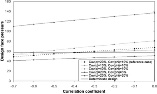
A reliability-based design 共RBD兲 has been performed in this sec-tion. It consists of the calculation of the required tunnel face pressure for a target collapse reliability index of 3.8 as suggested by Eurocode 7 for the ULS. This tunnel pressure is called here-after “probabilistic tunnel pressure.”

Fig. 18 presents the probabilistic tunnel pressure for different values of the coefficients of variation of the shear strength param-eters and their coefficient of correlation when the random vari-ables follow normal distributions. This figure also presents the deterministic tunnel face pressure 共56.6 kPa兲 corresponding to a safety factor against collapse 共Fs= ␴t/␴c兲 equal to 2. The

probabilistic tunnel face pressure decreases with the decrease of the coefficients of variation of the shear strength parameters and the increase of the negative correlation between these param-eters. It can become smaller than the deterministic tunnel face pressure for some values of the soil variability 共i.e., COV_␸= 5%, COV_c= 20%兲. However, for high values of the coefficients of variation, the required tunnel face pressure is much higher than

the deterministic value. As a conclusion, the deterministic tunnel face pressure may be higher or lower than the reliability-based tunnel face pressure, depending on the uncertainties of the ran-dom variables and the correlation between these variables.

Conclusions

A reliability-based analysis and design of the face stability of a shallow circular tunnel driven by a pressurized shield was per-formed. Only the collapse and the blow-out failure modes of the ULS were studied. Two rigorous deterministic models based on the upper-bound method of limit analysis were used. It was shown that

• Although the results given by the upper-bound approach in limit analysis are unsafe estimates of the collapse and blow-out loads, they are the best ones compared to the available solutions in both the active and passive cases. This is because the present mechanisms provide greater solutions than those given by Leca and Dormieux 共1990兲 in the collapse case and smaller results than those of these writers in the case of blow-out.

• The blow-out mode of failure does not occur for the cases currently encountered in practice. Hence, only the collapse failure mode was considered in the probabilistic analysis and design against face stability.

• The present limit analysis results obtained from the M1 col-lapse mechanism are not very far from the solutions given by complex 3D numerical simulations using FLAC3D_.

• The collapse reliability index increases with the increase of the tunnel face pressure.

• FORM approximation is an acceptable approach for estimating the failure probability against collapse for the commonly used values of the soil variability.

• The assumption of uncorrelated shear strength parameters was found conservative 共i.e., it gives a greater failure probability兲 in comparison to that of negatively correlated parameters; however, the type of the probability distribution does not sig-nificantly affect the values of the failure probability.

• The failure probability is more sensitive to ␸ than to c. The greater the scatter in ␸, the higher the failure probability. This means that the accurate determination of the uncertainties of the angle of internal friction ␸ is important in obtaining reli-able probabilistic results.

• When no correlation between shear strength parameters is con-sidered, a more spread out CDF of the tunnel pressure was obtained in comparison to the case of correlated shear strength parameters.

• The distribution of the PDF of the tunnel pressure was found very close to a lognormal distribution. This allows one to eas-ily determine the failure probability against collapse for a given face pressure.

• A RBD has shown that the tunnel pressure determined proba-bilistically decreases with the increase of the negative correla-tion between the shear strength parameters and the decrease of their coefficients of variation.

Appendix. Computation of the Tunnel Collapse Pressure—M1 Mechanism

The formulation is given here for a five-block mechanism. The formulation for another number of blocks is straightforward.

Fig. 16. PDFs of the tunnel face pressure

Fig. 17. Fit of the PDF of the tunnel pressure in the normal

uncor-related case

(13)

Geometry

The distance from the extremity of each block i to the tunnel crown共h_i兲 and the height of the extremity of the last block 共h₅_⬘兲 are given by 关Fig. 2共a兲兴

h5⬘= h5· sin共2␤4+ 2␤2+ ␣ − ␸兲 cos共⌿4,5− ␸兲 −

冉

H−D 2

冊

共19兲 with

冦

h2= D · cos共␣ + ␸兲 · cos共␤1− ␣ + ␸兲 sin共2␸兲 hi= h2·

兿

k=2 i−1

冋

cos共⌿k,k+1+ ␸兲 cos共⌿k−1,k− ␸兲

册

for i 艌 3

冧

共20兲

The volumes of the extreme blocks 共first and fifth blocks兲 are

V1= A1· h1− A1,2· h2 3 共21兲 V5= A4,5· h5− A5· h5⬘ 3 共22兲

The volume of an intermediate block i 共for 2 艋 i 艋 4兲 is

Vi=

Ai−1,i· hi− Ai,i+1· hi+1

3 共23兲

If h₅⬘⬎0, the value of the outcropping surface of the fifth block is A5= ⌸ cos共␸兲·

冉

h5⬘· sin共2␸兲 2 sin共2␤4+ 2␤2+ ␣ + ␸兲 · sin共2␤4+ 2␤2+ ␣ − ␸兲

冊

2 ·

冑

sin共2␤4+ 2␤2+ ␣ + ␸兲 sin共2␤4+ 2␤2+ ␣ − ␸兲共24兲 Otherwise, the mechanism does not outcrop and A5= 0.

The area of the elliptical surface resulting from the intersection of the first cone 共adjacent to the tunnel face兲 with the circular tunnel face is

A1= ⌸· D2

4 cos共␸兲·

冑

cos共␣ − ␸兲 · cos共␣ + ␸兲共25兲

The area of the contact elliptical surface between two successive blocks i and i + 1 is given by

冦

A1,2= ⌸· D2 4 cos共␸兲· cos共␣ + ␸兲 2_·

冑

cos共␤1− ␣ + ␸兲 cos共␤1− ␣ − ␸兲1.5 Ai,i+1= ⌸· D2 4 cos共␸兲· cos共␣ + ␸兲 2_·

冑

cos共⌿i,i+1+ ␸兲 cos共⌿i,i+1− ␸兲1.5 ·

兿

k=2 i

冋

cos共⌿k−1,k+ ␸兲2 cos共⌿k−1,k− ␸兲

册

for i 艌 2

冧

共26兲 Kinematics

The velocity of the block i and the relative velocity between the blocks i and i + 1 are

v_i=v₁·

兿

k=2 i cos共⌿k−1,k+ ␸兲 cos共⌿k−1,k− ␸兲 for i 艌 2 共27兲

v_i_,i+1=v_i· sin共2⌿i,i+1兲

cos共⌿i,i+1− ␸兲

for i 艌 1 共28兲

where

再

⌿0,1= ␣

⌿_i,i+1= ␤i− ⌿i−1,i for i 艌 1

冎

共29兲

Fig. 18. Comparison between deterministic and probabilistic design pressures

(14)

Expressions of N␥ and Ns

For a five-block collapse mechanism, the critical collapse pres-sure can be calculated from Eqs. 共10兲 and 共11兲, with

N␥= P31+ P41+ P51+ P52 D 共30兲 Ns= v₅ v₁ · sin共2␤2+ 2␤4+ ␣兲 · A5 A1· cos共␣兲共31兲 where P51= v₄ v₁· sin共2␤1 + 2␤3− ␣兲 · V4 A1· cos共␣兲共32兲 P52= v₅ v₁ · sin共2␤2+ 2␤4+ ␣兲 · V5 A1· cos共␣兲共33兲 P41= v₂ v₁ · sin共2␤1− ␣兲 · V2+ v₃ v₁ · sin共2␤2+ ␣兲 · V3 A1· cos共␣兲共34兲 P31= V1· sin共␣兲 A1· cos共␣兲共35兲 References

Baecher, G. B., and Christian, J. T. 共2003兲. Reliability and statistics in

geotechnical engineering, Wiley, New York.

Bhattacharya, G., Jana, D., Ojha, S., and Chakraborty, S. 共2003兲. “Direct search for minimum reliability index of earth slopes.” Comput.

Geo-tech., 30, 455–462.

Chen, W. F. 共2008兲. Limit analysis and soil plasticity, J. Ross Publishing Classics, 637.

Christian, J., Ladd, C., and Baecher, G. 共1994兲. “Reliability applied to slope stability analysis.” J. Geotech. Eng., 120共12兲, 2180–2207. Der Kiureghian, A., and Liu, P. L. 共1986兲. “Structural reliability under

incomplete probability information.” J. Eng. Mech., 112共1兲, 85–104.

Ditlevsen, O. 共1981兲. Uncertainty modelling: With applications to

multi-dimensional civil engineering systems, McGraw-Hill, New York. Fenton, G. A., and Griffiths, D. V. 共2003兲. “Bearing capacity prediction of

spatially random C-␸ soils.” Can. Geotech. J., 40, 54–65.

Haldar, A., and Mahadevan, S. 共2000兲. Probability, reliability and

statis-tical methods in engineering design, Wiley, New York.

Hasofer, A. M., and Lind, N. C. 共1974兲. “Exact and invariant second-moment code format.” J. Engrg. Mech. Div., 100共1兲, 111–121. Leca, E., and Dormieux, L. 共1990兲. “Upper and lower bound solutions for

the face stability of shallow circular tunnels in frictional material.”

Geotechnique, 40共4兲, 581–606.

Lemaire, M. 共2005兲. Fiabilité des structures, Hermès, Lavoisier, Paris 共in French兲.

Low, B. K., Lacasse, S., and Nadim, F. 共2007兲. “Slope reliability analysis accounting for spatial variation.” Georisk: Assessment and

manage-ment of risk for engineered systems and geohazards, 1共4兲, Taylor & Francis, London, 177–189.

Low, B. K., and Tang, W. H. 共1997a兲. “Efficient reliability evaluation using spreadsheet.” J. Eng. Mech., 123共7兲, 749–752.

Low, B. K., and Tang, W. H. 共1997b兲. “Reliability analysis of reinforced embankments on soft ground.” Can. Geotech. J., 34, 672–685. Low, B. K., and Tang, W. H. 共2004兲. “Reliability analysis using

object-oriented constrained optimization.” Struct. Safety, 26, 69–89. Melchers, R. E. 共1999兲. Structural reliability analysis and prediction, 2nd

Ed., Wiley, New York.

Mollon, G., Dias, D., and Soubra, A-H. 共2009兲. “Probabilistic analysis of circular tunnels using a response surface methodology.” J. Geotech.

Geoenviron. Eng., 135共9兲, 1314–1325.

Oberlé, S. 共1996兲. “Application de la méthode cinématique à l’étude de la stabilité d’un front de taille de tunnel, Final Project Rep. Prepared for

ENSAIS, Strasbourg, France 共in French兲.

Phoon, K.-K., and Kulhawy, F. H. 共1999兲. “Evaluation of geotechnical property variability.” Can. Geotech. J., 36, 625–639.

Rackwitz, R., and Fiessler, B. 共1978兲. “Structural reliability under com-bined random load sequences.” Comput. Struct., 9共5兲, 484–494. Soubra, A.-H. 共1999兲. “Upper-bound solutions for bearing capacity of

foundations.” J. Geotech. Geoenviron. Eng., 125共1兲, 59–68. Youssef Abdel Massih, D. S. 共2007兲. “Analyse du comportement des

fondations superficielles filantes par des approches fiabilistes.” Ph.D. thesis, Université of Nantes, Nantes, France 共in French兲.

Youssef Abdel Massih, D. S., and Soubra, A.-H. 共2008兲. “Reliability-based analysis of strip footings using response surface methodology.”

Int. J. Geomech., 8共2兲, 134–143.

Youssef Abdel Massih, D. S., Soubra, A.-H., and Low, B. K. 共2008兲. “Reliability-based analysis and design of strip footings against bear-ing capacity failure.” J. Geotech. Geoenviron. Eng., 134共7兲, 917–928.