Metaheuristics as a solving approach for the infrared heating in the thermoforming process
K. Bachir Cherif, D. Rebaine, F. Erchiqui, I. Fofana
G–2015–139 December 2015
Les textes publi´es dans la s´erie des rapports de recherche Les Cahiers du GERAD n’engagent que la responsabilit´e de leurs auteurs.
La publication de ces rapports de recherche est rendue possible grˆace au soutien de HEC Montr´eal, Polytechnique Montr´eal, Universit´e McGill, Universit´e du Qu´ebec `a Montr´eal, ainsi que du Fonds de recherche du Qu´ebec – Nature et technologies. D´epˆot l´egal – Biblioth`eque et Archives nationales du Qu´ebec, 2015.
The authors are exclusively responsible for the content of their research papers published in the series Les Cahiers du GERAD. The publication of these research reports is made possi-ble thanks to the support of HEC Montr´eal, Polytechnique Montr´eal, McGill University, Universit´e du Qu´ebec `a Montr´eal, as well as the Fonds de recherche du Qu´ebec – Nature et tech-nologies.
Legal deposit – Biblioth`eque et Archives nationales du Qu´ebec, 2015.
GERAD HEC Montr´eal 3000, chemin de la Cˆote-Sainte-Catherine Montr´eal (Qu´ebec) Canada H3T 2A7
T´el. : 514 340-6053 T´el´ec. : 514 340-5665 info@gerad.ca www.gerad.ca
approach
for
the
infrared
heating in the thermoforming
process
Kahina Bachir Cherif
aDjamal Rebaine
bFouad Erchiqui
cIssouf Fofana
aaGERAD & D´epartement des sciences appliqu´ees,
Uni-versit´e du Qu´ebec `a Chicoutimi, Saguenay (Qu´ebec) Canada, G7H 2B1
b GERAD & D´epartement d’informatique et de
math´ematique, Universit´e du Qu´ebec `a Chicoutimi, Saguenay (Qu´ebec) Canada, G7H 2B1
c Ecole de g´´ enie, Universit´e du Qu´ebec en Abitibi-T´emiscamingue, Rouyn-Noranda (Qu´ebec) Canada, J9X 5E4 kahina.bachir-cherif1@uqac.ca djamal rebaine@uqac.ca fouad.erchiqui@uqat.ca issouf fofana@uqac.ca December 2015
Les Cahiers du GERAD G–2015–139
Abstract: Thermoforming process is a technique widely used in the plastic industry. This process involves three stages: i) sheet heating, ii) forming, and iii) cooling and solidification. A crucial problem occurring during this process is the non-uniform distribution of the energy flux intercepted by the plastic sheet during infrared heating. To circumvent the occurring of this phenomenon, the approach that we followed is first model the heat process as an optimization problem. Then, two meta-heuristic algorithms, simulated annealing and migrating bird optimization algorithms, are applied and compared so as to meet as much as possible the corresponding objective function. An experimental study is then conducted to evaluate the quality of the solutions produced by both algorithms. Results are presented and analysed.
Key Words: Infrared heating, migrating bird optimization, simulated annealing, thermoforming process.
Acknowledgments: This research was partially financed for Djamal Rebaine, Fouad Erchiqui and Issouf Fofana by the Natural Sciences and Engineering Research Council of Canada (NSERC), and, for Kahina Bachir Cherif, by the Group for research in decision analysis (GERAD) and NSERC.
1
Introduction
Sheet thermoforming is widely used in the plastic industry. This process involves three stages: i) reheat: the initial polymeric sheet is oven-heated to a softened state using radiative heat transfer, ii) forming: the heated sheet is deformed into the mold under the action of air flow, and iii) cooling and solidification: the polymeric sheet cools in the mold. Temperature and deformation distribution in the final container can be predicted using a robust modelling of the energy and momentum equations (see e.g. Wiesche et al. [8]).
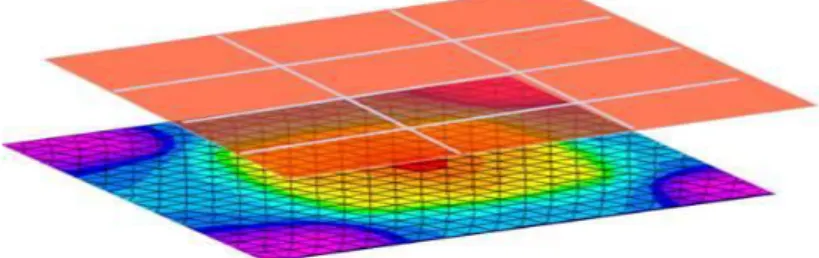
When heated by infrared radiation, the plastic sheet is transformed from glassy into a rubbery state. This hot state combined with the gravity creates a non-uniform thickness distribution in the plastic sheet. Adequate optimization of the heating stage can improve significantly the mass distribution in the finished part. One effective way to achieve better uniform thickness distribution is to reduce the differences of energy intercepted and absorbed by the different areas of the thermoplastic sheet. An illustration is pictured by Figure 1, in which the colours represent the intensity of energy received by the thermoforming sheet:
Figure 1: Distribution of energy received by a thermoplastic sheet from an infrared source
The classical methods of optimization of thermoplastics radiation have been the subject of many studies in the literature in finding the optimum solution of continuous and differentiable functions (see e.g. Boutaous et al. [1]). These methods are analytical in the sense that they make use of the techniques of differential calculus to locate optimum points. However, practical problems usually involve objective functions that are not continuous, nor differentiable. Therefore, the classical optimization techniques have a limited scope for those applications. One way to circumvent this difficulty is to discretize the problem so one can use iterative processes to rapidly produce reasonable solutions, but without the optimality guaranty.
The present paper is organized as follows. Section 2 introduces the problem we are considering. In Sec-tion 3, we present in an informal way the corresponding optimizaSec-tion formulaSec-tion that we derived for the problem we are considering. In Section 4, we highlight two meta-heuristic algorithms viz. the simulated annealing and the migrating bird optimization algorithms. Section 5 first presents details on the implemen-tation issues for both algorithms, and then results of the comparison study we conducted on the quality of the solutions produced by both algorithms.
2
Problem description
In the thermoforming process, the thermoplastic sheet is heated and formed in a mold through application of heat and pressure. The pressure is applied by introducing a vacuum, compressed air, or matched molds. Ceramic and quartz radiators are the main radiation sources used in an industrial scale thermoforming machines to heat plastic sheets. In the case of ceramic radiators, the entire mass of the system is maintained at a temperature of 570K–950K. On the other hand, quartz radiator systems use incandescent coils, including fused silica radiators with a coil temperature of 1200K, quartz glass radiators (1200K), and halogen radiators (2500K). Generally, the oven has a heater bank of n ceramic elements. The illustration of this process is pictured by Figure 2.
The incident radiation Qji on cell i of the thermoplastic sheet surface Si is calculated according to the
geometric orientation of surface Sj and temperature t of oven heater cell j. View factors are required to
Figure 2: The thermoforming (heating) process
that surface Sj of the heater is separated by a transparent medium from surface Si of the thermoplastic
sheet, the amount of radiation Qji leaving area Sj and reaching area of Si is given by the following equation
(see e.g. Erchiqui et al. [5]):
Qji = Fij
Sj
Si
σεt4. (1)
Parameter Fij denotes the view factor, ¯ε is the average source emissivity of the material. Parameter σ is the
Stefan-Boltzman of value 5.67 10−8 W/m2K, and t represents the temperature from the temperature set τ
assigned to cell j.
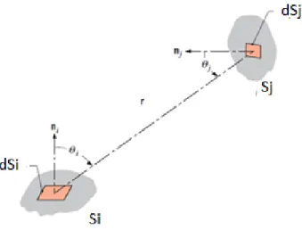
The view factors, given by the following Fij = 1 Si Z Si Z Sj cos θicos θj π × r2 dSidSj, (2)
are required to calculate the energy on the thermoplastic surface exposed to the infrared source. Note that, as illustrated by Figure 3, θi and θj are angles formed by the distance vector −→r and the normal vector −→n1
(respectively −n→2). Parameter r is the distance separating surface dSi and dSj.
Figure 3: Geometric definition of the view factor
Note that the evaluation of the double integrals of (2) is estimated with the numerical Gaussian integration method (see e.g. Dhatt and Touzot [3]).
3
Statement of the optimization problem
Before proceeding into the modelling process, let us recall that the energy received by each cell of the ther-moplastic sheet from a single heating cell is given by (1). The criterion that evaluates a uniform distribution
of the energy received by the thermoplastic sheet may be constructed as follows. The difference of energy received by two elements of the thermoplastic plastic sheet has an important influence on the quality of the final form of the product. Obviously, the smaller are the differences between these elements the better is the quality of the product. The goal is thus to make the elements of the thermoplastic sheet receive the same amount of heat from the heating elements. One may to achieve this goal is to minimize the standard deviation of the energy, compared to the mean, received by the cells of the thermoplastic sheet. To be more explicit, we proceed as follows. The expression of Qji may be written, for a given temperature τk to choose
from τ = (τ1, ..., τq), as
Qji = Fij
Sj
Si
εστk4.
It follows that the total energy received by cell i of the thermoplastic sheet is Ei= m X j=1 Qji. If x = 1 n n P i=1
Ei, then the goal is to minimize
1 x v u u t n X i=1 (Ei− x) 2 , (3)
such that any cell of the heating oven receives exactly one temperature from set τ , and a temperature from τ may be used at most m times.
Let us first make the following point about the objective function. The above problem was the subject of the work presented in Erchiqui et al. [5], and Nahas et al. [6]. The objective function they studied is similar to the one presented in (3), but without the denominator x of the fraction. The weakness of that function is that its minimization tends to favour the small values of the temperature set as they produce small values for that objective function. We recall that the goal is to find a small value of the standard deviation, but in comparison to its mean; the value of a standard deviation of data distributions is meaningful only when compared to its mean. In other words, what matters is the distribution of the values around their mean value, not the value of the standard variation on its own. This is the main reason the denominator appears in (3).
As stated, the above optimization problem is an extended version of the quadratic assignment problem. Indeed, the problem we are considering here may be viewed as seeking a mapping (and not a permutation as it is in the classical quadratic assignment problem) between the set of the temperatures and the set of the oven cells such that (3), a quadratic objective function, is minimized. It is known that the quadratic assignment problem is NP-hard (see e.g. Burkard et al. [2]). Therefore, the approximation approach is well justified as a solving method.
4
Metaheuristic approach
In this section, two meta-heuristic algorithms, simulated annealing and migrating bird optimization algo-rithms, are developed as a solving approach to distribute uniformly the energy intercepted by the material sheet.
4.1
The simulated annealing method
The simulated annealing (SA) approach is a technique that uses the analogy of a metal cooling until a minimum crystalline energy is reached. The goal is to bring a system from an arbitrary initial state to a state with a minimum possible energy.
In the implementation we designed we added two parameters. The first, the variable I, allows the exit from a given temperature if the solution is not improved after a certain number of successive iterations.
The second, parameter J, is another counter that permits the algorithm to stop if the current solution is not improved after a certain number of successive temperatures. The simulated annealing algorithm we implemented is resumed as below; for more details, see e.g. Pibouleau et al. [7].
1. Generate an initial solution S, and initialize T and c(0 < c < 1).
2. Set the maximum number of iterations iter-max, the maximum number U of successive temperatures T the current solution is not improved, the successive number I of times the current solution is not improved for a given T .
a. Generate a new ´S in the neighborhood of S and 4f = fS− fS´;
b. if 4f > 0 then S ← ´S;
else { - generate at random r in [0,1]; - if r < exp (−4f /T )
S ← ´S }; c. Set T = T ∗ c if I is reached;
3. Repeat Step 3 until either iter-max or U is reached.
The neighbourhood utilized for the above version of SA is as follows: Procedure Neighborhood {
1. Generate at random r in [0,1]; 2. if (r < 0.5)
Select at random two temperature locations i and j from the actual solution, and then exchange the two corresponding temperatures;
else Select at random a temperature location i from current solution S, and choose at random a temperature t from τ and assign it to cell i.
} // end of the procedure
This technique of exploring the neighbourhood space allows a certain diversification. Indeed, if a solution cannot be improved with the permutation of the actual temperatures, then a new temperature from the temperature set is generated to replace a temperature of an arbitrary cell.
4.2
The migrating bird optimization method
The Migration Birds Optimization (MBO) was recently introduced by Ekram et al. [4]. Their method is inspired from the shape of the flight in ‘V’ of the migrating birds. The property of bird flights lies mainly in the energy conservation. Indeed, when a bird beats its wings, it generates a draft which will make the birds behind supplying fewer efforts to rise. The organization of the flight of birds is as follows: the bird at the head leads the group for a certain period, and spends more energy than the rest of the birds. When it gets tired, it moves to the back of the group, and one of the birds behind takes the lead. The idea behind the algorithm that one may derive works as follows. The leader is chosen according to the best performance. At first, we select the best solution among the set of the solutions generated previously as initial solutions. Then, two lists are created, a left and a right list, to form the V-shape of the flight as follows: the first solution is added to the left list, the second in the right list, and so on until all the solutions are placed. This way of placing the solutions is similar to that of birds. Indeed, the strongest bird is placed forward, whereas the least strong are placed behind, among others the old birds (see Figure 4 for an illustration).This way of arranging the solutions may lead in the search for the best solution to more promising regions and find the solution we are looking for in a reasonable laps of time.
As the method is quite recent, let us detail its description. For the sake of clarity, we first start mentioning analogies between MBO and natural bird migration. This makes it easy to justify the approach.
Figure 4: V-shape of bird flights
MBO Flight of migrating birds
Number of solutions P Nombre of birds
Number α of evaluated neighbors Induced strength that is required Number β of shared neighbors Distance between birds
Number x of iterations Flight time of the leader bird The parameters defining the above algorithm are thus as follows:
• P = the number of initial solutions.
• α = the number of neighbor solutions to consider.
• β = the number of neighbors to share with the next solution.
• x = the number of iterations to perform before changing the leader solution, and • K = the maximum number of iterations the algorithm executes.
The MBO algorithm mainly consists of four phases summarized as follows:
Step 1: This step initializes the parameters of the algorithm. First, it is recommended to choose P as an odd number in order to have the same number of solutions in the two lists in addition to the bird leading the flock. The number α of generated neighbors to evaluate may be interpreted as the necessary power of the flight. This power is inversely linked to the speed. With a bigger α, the birds flight at lower altitude, which helps to explore the neighborhood in details. By generating a large number of neighbors, we better explore the search space. Birds behind get less tired compared with those who are forwards, and thus save more energy. To respect this property in the MBO algorithm, we use the mechanism of services between the solutions. For the solutions at the back of the flock, through β the number of neighbors to share with the next solution, by generating fewer neighbors and by using the neighbors of the solutions in front, the algorithm can respect the property of energy conservation. Finally, the number x of iterations, before changing the solution linked to the leader at the head of the flock, represents the time spent by the leader of the group before its replacement.
Step 2: To improve the leading solution, α neighbour solutions are randomly generated. If the best neighbour solution is better than the leader, the latter is replaced by this solution, otherwise, it remains unchanged. The (α − 1) neighbour solutions not used by the leader solution are sorted in increasing order according to their objective values. Then, two groups, one is at the left and the other one is at the right, are formed as follows: the first and the second neighbour solution are added into the left and right lists, respectively, and so on. Let us note that each of these two sets is of cardinality β.
Step 3: The process of improvement progresses along the lists of the frock towards the tail. For a solution in the left list, we generate (α − β) randomly solutions in its neighbourhood. Then, these solutions are evaluated. The best solution is used to improve the current solution. The process is repeated until all the
solutions in the left list are evaluated and possibly improved. The same procedure is used for the solutions in the right list. This procedure is repeated x times without changing the leader.
Step 4: we proceed in this step to the change of the leader solution. The procedure is similar to what make the real birds: the bird spending most energy moves back behind for a rest, and another bird will take the lead. By analogy, the leading solution is alternately moved into the extremities of the left and the right line of both lists and the first solution of the list where the leader was placed is passed on as the new leader. With this mechanism, a solution which does not succeed in improving itself with its own neighbours is replaced by one of the neighbours of the previous solution, if the previous solution is naturally more promising. In this way, the region around the most promising solution will be explored more in details.
The steps followed an MBO algorithm may be then resumed as below: Procedure MBO {
1. Fix P, α, β, x and K (the maximum number of iteration MBO executes). 2. Generate arbitrarily n solutions, and place them in a V-shape.
3. Improve the leader solution by generating and evaluating α of its neighbors.
4. Improve the solution in the V-shape by evaluating (α − β) neighbors with the β best solutions not used in the solution ahead.
5. Repeat x times Step 2 and 3.
6. Move the leader to the back of the group, and move one of the next solutions that are behind it to the leader position.
7. If K is not reached, repeat Step 2 until Step 6. } // end of the procedure.
5
Experimental study
This section describes the experiments that we conducted to compare the two proposed algorithms (SA and MBO). We limited this comparison to the quality of the solutions they produced by setting the number of evaluated solutions to a maximum value of 10 000. The characteristics of the thermoforming device are as follows. The number of the oven heating cells is fixed to 36 (6 × 6) elements. The size of the heating cells is 1.2 × 1.8mm. The size of the thermoplastic sheet is 1 × 1.6mm, and the distance that separates the thermoplastic sheet and the heating oven is fixed to 1m. The average emissivity ¯ε of the thermoplastic sheet is set to 0.8.
The two algorithms are implemented in Matlab, version 7.12.0 (R2012a), and executed on an INTEL 2.0 GHz Dual Core processor with a RAM of 8192 MB capacity. Let us also mention that each execution of both algorithms is done on 10 instances generated arbitrarily. The values of the temperature set, we used in each simulation, are drawn from the interval [400, 900].
We first conducted experiments to tune the parameters of SA and MBO. Then, we compared the quality of both algorithms on several types of instances.
5.1
Parameters tuning
In this section, we present the study we conducted on tuning the different parameters related to the simulated annealing and the migrating bird optimization algorithms.
The parameters of the simulated annealing that we focused on are the initial solution, the initial temper-ature, the decrease of the tempertemper-ature, and the number of iterations. Except the initial solution, our choice for the rest of the parameters is based on those utilized in Nahas et al. [5] as follows:
2. The decrease of T obeys the following updating T = T × c, where c = 0.99.
3. The number of successive iterations without an improvement on the objective for a given temperature is set to I = 40.
4. The number of successive temperatures without an improvement on the objective function is set to U = 40.
With regard to the initial solution, we tested the following rules:
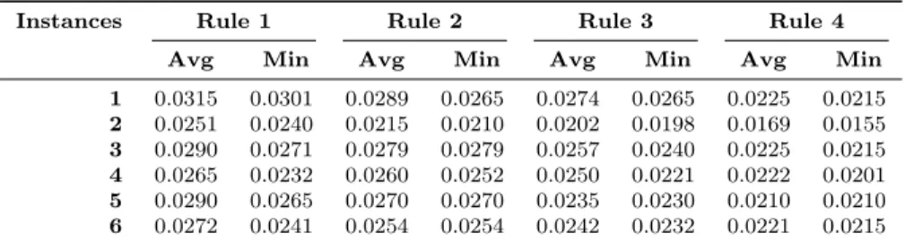
• Rule 1: fix each cell to an arbitrary temperature from the temperature set. • Rule 2: fix the cells to an arbitrary temperature from the temperature set. • Rule 3: fix the cells to the minimum temperature from the temperature set. • Rule 4: fix the cells to the maximum temperature from the temperature set. The results we got are summarized by Table 1.
Table 1: Selecting an initial solution for the simulated annealing algorithm
Instances Rule 1 Rule 2 Rule 3 Rule 4
Avg Min Avg Min Avg Min Avg Min
1 0.0315 0.0301 0.0289 0.0265 0.0274 0.0265 0.0225 0.0215 2 0.0251 0.0240 0.0215 0.0210 0.0202 0.0198 0.0169 0.0155 3 0.0290 0.0271 0.0279 0.0279 0.0257 0.0240 0.0225 0.0215 4 0.0265 0.0232 0.0260 0.0252 0.0250 0.0221 0.0222 0.0201 5 0.0290 0.0265 0.0270 0.0270 0.0235 0.0230 0.0210 0.0210 6 0.0272 0.0241 0.0254 0.0254 0.0242 0.0232 0.0221 0.0215
We have generated six different instances to compare the performance of the above rules. The results we got are summarized in Table 1, and pictured in Figure 5. We observed that Rule 2 generates better results than the rest. Therefore, in the simulated annealing we implemented, the initial solution is generated by Rule 2.
Figure 5: Minimal and average values of the objective function
With regards to MBO algorithm, we had to conduct a complete experimental study for the choice of the main parameters P, α, β, x and K. Let us first start with the initial solutions. Since MBO algorithm is a metaheuristic with a population, and in order to start the algorithm with a certain level of diversity, we generated initial solutions arbitrarily from a uniform distribution.
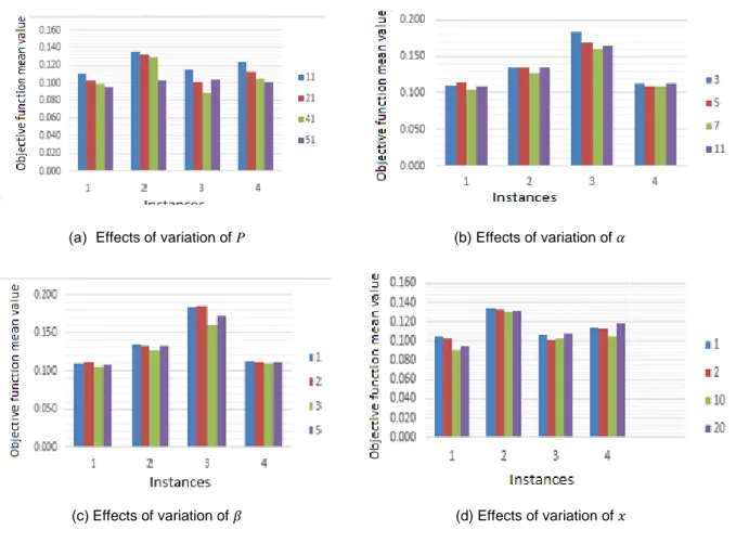
In Ekram et al. [4], it was recommended to set n to an odd number with a modest value. We tested our algorithm for n in the range 11 to 51. As shown by Figure 6a, we got better solution for P = 51. We tested α for modest values so as to explore a large number of solutions in the neighborhood of a solution. Our tests for α = 3, 5, 7, 11, and 21, as resumed in Figure 6b, show that the results as much better for α = 7.
Again, Ekram et al. [4] recommended choosing small values for β. The values we selected for our tests are β = 1, 2, 3, and 5. The results we got, as resumed in Figure 6c, suggest the value β = 3. Again, it was recommended in Ekram et al. [4] to choose a modest value for x. We conducted a simulation for x = 1, 2, 10 and 20. As resumed in Figure 6d, the results are better for x = 10. In the following, the abbreviations avg and Std mean average and standard deviation, respectively.
(a) Effects of variation of P (b) Effects of variation of 𝛼
(c) Effects of variation of 𝛽 (d) Effects of variation of 𝑥
Figure 6: Analysis to determine the value of the parameters MBO
5.2
Simulated annealing vs. migrating bird optimization
This section is devoted to the comparison of the two metaheuristics under study viz. simulated annealing and migrating bird optimization.
The different pairs (n, m) that we used, in the simulation we conducted to build the temperature set from which we select the temperatures to heat up the cell of oven, are follows:
Case 1. n = mn = mn = m: The number of temperatures generated is the same as the number of the cells in the infrared oven.
Case 2. n > mn > mn > m: The number of temperatures generated arbitrarily is less than the number of the cells of the infrared oven. We distinguished three subcases: n = 1
4m, n = 1
2m, n = 3 4m.
Case 3. n < mn < mn < m: The number of temperatures generated arbitrarily is greater than the number of the cells of the infrared oven. We distinguished three subcases: n = 32m, n = 2m, n = 52m.
In the following, we present for the different cases, presented above, the results produced by SA and MBO and the best solution, in terms of selected temperatures assigned to the oven cells, generated by each approach, followed the corresponding energy flux received by the cells of the thermoforming sheet, respectively. We executed both algorithms 10 times for each set t of temperatures generated randomly.
Case 1. n = m = 36n = m = 36n = m = 36. The temperature set is as follow, and the results are as in Table 2:
τ = {518, 589, 585, 619, 594, 489, 441, 826, 565, 732, 892, 506, 665, 443, 800, 851, 457, 842, 773, 537, 879, 834, 491, 847, 790, 463, 796, 691, 406, 460, 417, 760, 554, 403, 617, 605}
Table 2: Results produced by SA and MBO
1 2 3 4 5 6 7 8 9 10 Avg Std
MBO 0.059 0.059 0.058 0.057 0.057 0.053 0.055 0.058 0.057 0.053 0.057 0.002 SA 0.041 0.043 0.041 0.042 0.040 0.040 0.041 0.040 0.043 0.041 0.041 0.001
Table 3: Distribution of the temperatures produced by SA 892 790 403 403 732 892 665 403 403 403 403 403 403 403 403 403 403 403 403 403 403 403 403 403 851 403 403 403 403 796 892 406 403 403 441 892
Table 4: The corresponding distribution energy flux received by the thermoplastic sheet
968.9 1044.8 1073.2 1066.9 1037.7 985.1 1027.6 1107.1 1137.8 1130.9 1097.5 1038.2 1005.7 1081.4 1113.2 1108.9 1076.5 1017.4 996.2 1066.9 1096.4 1093.3 1065.3 1012.7 1019.0 1084.9 1108.0 1103.1 1080.7 1038.2 1001.6 1061.2 1078.0 1071.7 1055.4 1023.6
Table 5: Distribution of the temperatures produced by MBO 851 619 537 585 589 691 619 892 506 443 403 665 417 460 585 491 554 506 619 460 443 489 665 800 463 589 892 457 619 506 790 460 879 760 417 417
Table 6: The corresponding distribution energy flux received by the thermoplastic sheet
1165.8 1291.1 1362.9 1381.1 1349.2 1267.8 1312.7 1450.9 1523.9 1531.0 1478.8 1373.4 1352.9 1488.1 1554.8 1551.4 1485.3 1366.4 1348.6 1477.0 1537.8 1529.7 1459.1 1335.7 1325.7 1450.2 1508.1 1499.1 1429.0 1305.3 1250.2 1366.8 1419.5 1410.0 1343.9 1226.4
Case 2. n < mn < mn < m. We investigate here three subcases according to the value of n as a function of m. Subcase 2.1. n =n =n =141414m = 9m = 9m = 9. The temperature set is as follows, and the results are as in Table 7. τ = {459, 649, 880, 570, 693, 512, 776, 527, 653}
Table 7: Results produced by SA and MBO algorithms
1 2 3 4 5 6 7 8 9 10 Avg Std
MBO 0.060 0.058 0.058 0.058 0.054 0.055 0.056 0.054 0.058 0.055 0.057 0.001 SA 0.049 0.049 0.049 0.049 0.051 0.049 0.051 0.048 0.049 0.049 0.049 0.001
Table 8: Distribution of the temperatures produced by SA 880 880 459 459 880 880 776 459 459 459 459 459 459 459 459 459 459 459 459 459 459 459 459 512 880 459 459 459 459 776 880 776 459 527 693 880
Table 9: The corresponding distribution energy flux received by the thermoplastic sheet
1285,3 1402,2 1456,3 1457,7 1417, 1334,8 1385,7 1507,2 1561,7 1558,6 1509,3 1415,4 1372,4 1487,1 1539,0 1534,7 1483,2 1388,3 1358,7 1466,9 1514,8 1509,5 1460,0 1370,0 1380,2 1485,7 1527,5 1518,4 1470,9 1387,1 1352,7 1454,4 1491,0 1479,6 1435,8 159,89
Table 10: Distribution of the temperatures pro-duced by MBO 857 808 716 808 808 539 808 463 463 857 879 857 673 673 808 448 879 463 808 673 857 853 857 857 539 808 463 716 808 463 539 673 448 673 673 673
Table 11: The corresponding distribution energy flux received by the thermoplastic sheet
1697.5 1897.3 2013.2 2031.9 952.93 1786.7 1881.0 2086.6 2196.1 2199.6 2101.7 1916.5 1906.9 2094.0 2182.9 2169.8 2064.0 1881.8 1869.1 2044.5 2124.2 2107.8 2006.8 1836.5 1810.5 1993.7 2085.4 2083.3 1996.8 1839.0 1676.7 1870.8 1983.3 2005.0 1939.8 1797.6
Subcase 2.2. n = 1 2m = 18
n =12m = 18 n = 1
2m = 18. The temperature set is as follows, and the results are as in Table 12.
τ = {796, 880, 728, 417, 825, 867, 740, 779, 772, 596, 728, 485, 753, 414, 538, 423, 448, 812} Table 12: Results produced by SA and MBO algorithms
1 2 3 4 5 6 7 8 9 10 Avg Std
MBO 0.059 0.058 0.058 0.056 0.055 0.053 0.056 0.058 0.059 0.057 0.057 0.002 SA 0.045 0.044 0.044 0.044 0.045 0.043 0.044 0.044 0.044 0.045 0.044 0.001
Table 13: Distribution of the temperatures pro-duced by SA 880 740 414 414 753 880 728 414 414 414 414 414 414 414 414 414 414 414 414 414 414 414 414 414 753 414 414 414 414 812 880 728 414 414 414 825
Table 14: The corresponding distribution energy flux received by the thermoplastic sheet
950.8 1025.6 1055.7 1053.5 1028.7 979.1 1019.1 1098.4 1130.4 1126.1 1095.2 1037.1 1000.0 1077.9 1112.1 1109.9 1078.5 1018.9 983.0 1058.8 1093.6 1093.6 1065.6 1010.5 1001.8 1075.9 1105.9 1102.6 1076.0 1026.0 997.1 1066.5 1087.8 1076.6 1047.3 1000.1
Table 15: Distribution of the temperatures pro-duced by MBO 423 867 825 448 812 867 753 728 423 417 740 812 728 538 796 423 796 596 753 867 415 779 596 740 880 417 538 417 740 596 728 414 414 485 596 796
Table 16: The corresponding distribution energy flux received by the thermoplastic sheet
1509.2 1673.8 1764.1 1775.8 1714.0 1585.8 1679.6 1848.4 1930.8 1926.4 1845.1 1697.8 1719.0 1874.8 1941.3 1921.3 1828.3 1676.2 1714.6 1861.4 1919.2 1893.1 1797.8 1647.2 1694.8 1844.2 1905.7 1884.8 1794.9 1648.2 1600.6 1754.3 1825.9 1817.7 1740.2 1602.7
Subcase 2.3. n =n =n =343434m = 27m = 27m = 27. The temperature set is as follows, and the results are as in Table 17:
τ = {596, 728, 485, 753, 415, 538, 423, 448, 812, 748, 558, 876, 417, 619, 591, 783, 798, 493, 645, 623, 723, 755, 778, 538, 740, 728, 481}
Table 17: Results produced by SA and MBO algorithms
1 2 3 4 5 6 7 8 9 10 Avg Std
MBO 0.059 0.060 0.059 0.061 0.056 0.057 0.056 0.060 0.061 0.059 0.059 0.002 SA 0.044 0.045 0.044 0.044 0.045 0.046 0.049 0.045 0.044 0.045 0.045 0.002
Table 18: Distribution of the temperatures pro-duced by SA 876 778 415 415 798 876 755 415 415 415 415 423 415 415 415 415 415 415 417 415 415 415 415 415 783 415 415 415 415 798 876 723 415 415 723 798
Table 19: The corresponding distribution energy flux received by the thermoplastic sheet
1019.2 1101.8 1136.1 1133.9 1105.4 1048.6 1092.5 1178.9 1213.5 1207.8 1171.9 1105.7 1071.0 1154.1 1189.6 1184.9 1147.6 1079.7 1050.3 1131.1 1167.3 1165.1 1131.4 1067.6 1067.5 1148.3 1182.3 1179.7 1149.2 1090.6 1059.0 1137.8 1167.6 1162.3 1133.4 1079.0
Table 20: Distribution of the temperatures pro-duced by MBO 755 448 728 755 645 623 740 591 619 728 723 596 753 728 755 493 723 448 740 481 753 596 558 728 493 415 876 778 493 485 485 481 740 728 415 778
Table 21: The corresponding distribution energy flux received by the thermoplastic sheet
1296.7 1448.7 1535.8 1548.8 1489.1 1364.9 1445.6 1605.4 1689.7 1692.5 1618.7 1478.8 1473.6 1623.8 1696.8 1689.2 1608.9 1468.2 1458.1 1601.8 1668.0 1655.0 1572.5 1434.1 1430.4 1575.7 1642.8 1629.9 1547.9 1411.0 1338.6 1482.2 1552.0 1544.8 1470.5 1342.3
Case 3. n > mn > mn > m. Again, we investigate three subcases according to the value of n as a function of m. Subcase 3.1. n =n =n =323232m = 54m = 54m = 54. The temperature set is as follows, and the results are as in Table 22:
τ = {808, 853, 463, 857, 716, 448, 539, 673, 879, 883, 478, 886, 879, 643, 800, 471, 611, 858, 796, 880, 728, 417, 825, 867, 740, 779, 772, 596, 728, 485, 753, 415, 538, 423, 448, 812, 748, 558, 876, 417, 619, 591, 783, 798, 493, 645, 623, 723, 755, 778, 538, 740, 728, 481}
Table 22: Results produced by SA and MBO
1 2 3 4 5 6 7 8 9 10 Avg Std
MBO 0.063 0.059 0.059 0.059 0.057 0.057 0.057 0.064 0.059 0.062 0.059 0.003 SA 0.043 0.044 0.044 0.043 0.040 0.043 0.043 0.043 0.043 0.050 0.044 0.002
Table 23: Distribution of the temperatures pro-duced by SA 886 853 415 415 800 886 716 415 415 415 415 418 415 415 415 415 415 415 415 415 415 415 415 417 883 415 415 415 415 783 886 558 415 415 716 883
Table 24: The corresponding distribution energy flux received by the thermoplastic sheet
1110,6 1203,4 1240,5 1234,2 1197,3 1130,4 1181,9 1277,9 1316,2 1308,3 1266,2 1191,8 1158,3 1248,2 1286,3 1280,3 1239,3 1165,9 1145,0 1229,1 1264,7 1260,4 1224,5 1158,1 1167,1 1248,1 1279,5 1275,6 1246,8 1190,6 1143,6 1221,1 1249,9 1248,9 1229,4 1185,1
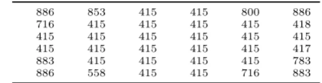
Table 25: Distribution of the temperatures pro-duced by MBO 645 858 800 755 481 858 558 539 623 886 728 418 539 493 463 723 853 728 876 858 591 867 596 880 716 478 783 886 728 596 673 591 417 812 596 853
Table 26: The corresponding distribution energy flux received by the thermoplastic sheet
1417.6 1588.8 1696.9 1732.7 1693.7 1581.9 1556.6 1746.7 1872.0 1922.6 1893.1 1781.4 1562.1 1744.4 1864.9 1914.9 1888.9 1783.6 1535.8 1704.4 1810.5 1847.8 1813.5 1707.2 1521.5 1687.1 1787.0 1815.4 1772.2 1659.8 1464.0 1631.0 1733.0 1762.7 1719.5 1607.1
Subcase 3.2. n = 2m = 72n = 2m = 72n = 2m = 72. The temperature set is as follows, and the results are as in Table 27:
τ = {522 865 575 498 525 708 637 576 816 693 675 859 543 779 777 590 684 438 427 665 790 867 465 684 635 405 568 481 797 555 664 482 701 531 727 745 774 625 441 514 857 476 813 669 899 439 621 453 881 402 788 809 835 442 600 530 800 616 856 491 532 472 468 835 690 675 472 827 711 575 657 807}
Table 27: Results produced by SA and MBO
1 2 3 4 5 6 7 8 9 10 Avg Std
MBO 0.064 0.063 0.064 0.062 0.063 0.062 0.061 0.068 0.064 0.063 0.063 0.002 SA 0.041 0.042 0.043 0.043 0.041 0.041 0.041 0.043 0.044 0.041 0.042 0.001
Table 28: Distribution of the temperatures pro-duced by SA 899 857 402 402 727 899 684 402 402 402 402 625 402 402 402 402 402 405 405 402 402 402 402 405 865 402 402 402 402 816 899 657 402 402 568 881
Table 29: The corresponding distribution energy flux received by the thermoplastic sheet
1422.2 1542.1 1590.3 1582.6 1535.5 1450.2 1523.6 1648.6 1699.1 1690.3 1638.0 1544.5 1494.5 1613.1 1664.3 1658.4 1607.3 1514.1 1469.9 1582.7 1632.0 1627.0 1578.5 1489.2 1497.4 1609.2 1653.2 1644.4 1596.8 1511.7 1483.6 1593.8 1633.0 1621.0 1575.9 1497.2
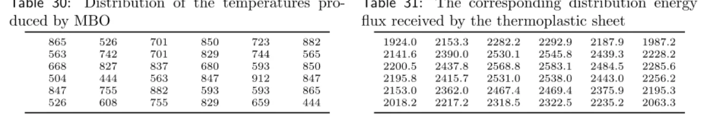
Table 30: Distribution of the temperatures pro-duced by MBO 865 526 701 850 723 882 563 742 701 829 744 565 668 827 837 680 593 850 504 444 563 847 912 847 847 755 882 593 593 865 526 608 755 829 659 444
Table 31: The corresponding distribution energy flux received by the thermoplastic sheet
1924.0 2153.3 2282.2 2292.9 2187.9 1987.2 2141.6 2390.0 2530.1 2545.8 2439.3 2228.2 2200.5 2437.8 2568.8 2583.1 2484.5 2285.6 2195.8 2415.7 2531.0 2538.0 2443.0 2256.2 2153.0 2362.0 2467.4 2469.4 2375.9 2195.3 2018.2 2217.2 2318.5 2322.5 2235.2 2063.3
Subcase 3.3. n =5 2m = 90
n = 52m = 90 n = 5
2m = 90. The temperature set is as follows, and the results are as in Table 32:
τ = {853 463 857 716 448 539 673 879 883 478 886 879 643 800 471 611 858 796 880 728 417 825 867 740 779 772 596 728 485 753 415 538 423 448 812 748 558 876 417 619 591 783 798 493 645 623 723 755 778 538 740 728 481 459 649 880 570 693 512 776 527 653 750 846 880 674 469 474 529 821 527 807 522 865 575 498 525 708 637 576 816 693 675 859 543 779 777 590 684 808}
Table 32: Results produced by SA and MBO algorithms
1 2 3 4 5 6 7 8 9 10 Avg Std
MBO 0.061 0.061 0.063 0.060 0.057 0.059 0.058 0.060 0.060 0.061 0.060 0.002 SA 0.042 0.043 0.043 0.042 0.042 0.043 0.042 0.043 0.043 0.044 0.043 0.001
Table 33: Distribution of the temperatures pro-duced by SA 886 415 415 415 796 886 693 415 415 415 415 527 415 415 415 415 415 415 415 415 415 415 415 415 880 415 415 415 415 858 886 693 415 415 448 886
Table 34: The corresponding distribution energy flux received by the thermoplastic sheet
1135,7 1233,0 1272,4 1265,9 1227,2 1157,9 1204,8 1305,5 1347,4 1341,3 1299,7 1224,9 1179,5 1273,8 1315,8 1313,2 1274,9 1203,3 1169,4 1257.0 1295,4 1293,7 1260,7 1197,4 1199.0 1281,8 1312,4 1306,5 1277,1 1222,9 1182,5 1259,5 1282,0 1271.2 1243,7 1197,2
Table 35: Distribution of the temperatures pro-duced by MBO 776 859 463 645 807 469 716 821 853 728 858 708 753 596 723 783 527 645 883 867 716 880 779 649 880 538 674 653 527 543 693 418 740 417 576 825
Table 36: The corresponding distribution energy flux received by the thermoplastic sheet
1817.8 2021.3 2123.8 2118.3 2018.1 1844.7 2013.6 2235.8 2349.0 2347.9 2246.7 2064.9 2040.7 2261.8 2381.6 2394.8 2310.6 2141.6 2008.6 2232.9 2365.0 2395.1 2325.1 2162.6 1963.1 2196.7 2341.9 2383.0 2315.8 2146.7 1837.7 2064.6 2208.9 2252.6 2188.0 2019.8
Table 37 summarizes the results obtained from the execution of two algorithms through the instances we have generated. We note that, on the seven generated instances, the best results are produced by the simulated annealing algorithm. Nevertheless, some remarks connected to the average and standard deviations of the generated results are to be made:
1. For the seven instances we have studied, the method of SA generates by far better results than MBO in terms of average and standard deviation for the values generated for the objective function.
2. The discrepancy between the cells in terms of energy received by the thermoplastic sheet is significant for MBO than for SA.
3. Even though this was not our primary goal for the comparison we conducted, we noticed that the running time of SA to generate a solution is much better than that of MBO, and
4. The convergence of MBO towards the best solution is very slow compared with SA.
Table 37: Results produced by SA and MBO algorithms for all the cases
MBO SA
N Min Avg Std Min Avg Std
9 0.054 0.057 0.001 0.048 0.049 0.001 18 0.053 0.057 0.002 0.044 0.044 0.001 36 0.053 0.057 0.002 0.041 0.041 0.001 54 0.057 0.059 0.003 0.043 0.044 0.002 72 0.061 0.063 0.002 0.041 0.02 0.001 90 0.058 0.060 0.002 0.042 0.043 0.001
We conclude not only from the above results related to the values of the objective function, but also by visualizing the distributions of the energy intercepted by the thermoplastic sheet generated by both algorithms, resumed by the above tableaux, that the simulated annealing algorithm clearly outperforms the migrating bird emigrating optimization method.
6
Conclusion
The study we conducted in this paper allowed us to adapt the MBO method for the resolution of a problem of thermoforming modelled in the form of a problem of combinatorial optimization, in this particular case, the problem of the quadratic assignment problem. Then, we conducted an extensive experimental study by first tuning the different parameters linked to SA and MBO, and by comparing the quality of the solution produced by these two algorithms.
This study reveals that the quality of the solutions generated by SA outperforms those of MBO in all the cases. Even from the running time point of view, this conclusion is still the same.
For further research, it would be interesting to design much more involved heuristics to generate an initial solutions and see to what extent this may influence not only the quality of the final solution, but also the convergence of the simulated annealing method. Different structures of neighborhood are also a good research avenue to improve the performance of SA.
On the other hand, we have suggested, through the expression of the objective function, another way of capturing the distribution of the energy flux received by the thermoforming sheet. Even though we improved the quality of this distribution, compared to the results generated by SA in Nehas et al. [6], we still observe significant discrepancies between cells as regards to the energy flux received by the thermoforming sheet. It would be of interest to improve the quality of this distribution by developing other objective functions. This avenue of research is in progress.
References
[1] Boutaous M., Bourgin P., Heng D., Garcia D. (2005) Optimization of radiant heating using the ray tracing method: Application to thermoforming.Journal of Advanced Sciences, 17(1/2), 139–135.
[2] Burkard R., Dell’Amico M., Martello S. (2012) Assignment Problems, revised reprint, SIAM.
[3] Dhatt G., Touzot G. (1984) Une pr´esentation de la m´ethode des ´el´ements finis, 2nd ´edition, Collection, Universit´e de Compi`egne.
[4] Ekram D., Mitat U., Ali Fuat A. (2012) Migrating bird optimization: A new metaheuristic approach and its performance on quadratic assignment problem. Information Sciences, 217, 65–77.
[5] Erchiqui F., Nahas N., Nourelfath M., Souli M. (2011) A metaheuristic algorithms for optimization of infrared heating stage of the thermoforming process. International Journal of Metaheuristics, 1(3), 199–221.
[6] Nehas, F. Bachir Cherif K., Rebaine D., Erchiqui F. (2015) A heuristic approach for the infrared heating in thermoforming process, submitted for publication.
[7] Pibouleau L., Domenech S., Davin A., Azzaro-Pantel C. (2005) Exp´erimentations num´eriques sur les variantes et param`etres de la m´ethode du recuit simul´e. Chemical Engineering Journal, 1(3), 117–130.
[8] Wiesche S.A. (2004) Industrial thermoforming simulation of automotive fuel tanks. Applied Thermal Engineer-ing, 24, 2391–2409.