Belhaj Hassine: Senior Economist, Economic Research Forum, PEP, Cairo, Egypt Robichaud: Researcher, Poverty and Economic Policy (PEP) Research Network
Decaluwé: Department of Economics, Université Laval, PEP, CIRPÉE, Quebec, Canada and CEPII, France Cahier de recherche/Working Paper 10-22
Agricultural Trade Liberalization, Productivity Gain and Poverty
Alleviation: a General Equilibrium Analysis
Nadia Belhaj Hassine Véronique Robichaud Bernard Decaluwé
Abstract:
Computable General Equilibrium (CGE) models have gained continuously in popularity as an empirical tool for assessing the impact of trade liberalization on agricultural growth, poverty and income distribution. Conventional models ignore however the channels linking technical change in agriculture, trade openness and poverty. This study seeks to incorporate econometric evidence of these linkages into a CGE model to estimate the impact of alternative trade liberalization scenarios on poverty and equity. The analysis uses the Latent Class Stochastic Frontier Model (LCSFM) and the metafrontier function to investigate the influence of trade openness on agricultural technological change. The estimated productivity effects induced from higher levels of trade are combined with a general equilibrium analysis of trade liberalization to evaluate the income and prices changes. These effects are then used to infer the impact on poverty and inequality following the top-down approach. The model is applied to Tunisian data using the social accounting matrix of 2001 and the 2000 household expenditures surveys. Poverty is found to decline under agricultural and full trade liberalization and this decline is much more pronounced when the productivity effects are included.
Keywords: Openness, Agriculture, Productivity, Poverty, CGE modeling
1. Introduction
The Uruguay Round commitments and the current Doha Round of agricultural trade talks have raised the interest in understanding how the trade reforms will impact the wellbeing of the poor.4 While agriculture continues to be the major stumbling block in the ongoing trade negotiations, a progress was made towards reaching a consensus on a road map for agricultural liberalization (Anderson and Martin, 2006). Agriculture is of major importance for the poor who rely on this sector for their main source of income and sustenance. Thus expanding the agricultural market access opens up opportunities for developing the farming sector and offers scope for bettering the livelihoods of the poor, but it can also cause them many hardships (Hertel and Reimer, 2005; Bardhan, 2006; Hertel, 2006). The agricultural reforms have sparked a fervent debate about whether the removal of trade protection benefits the poor or not. While there is a great deal of empirical support for the poverty-alleviation potential of trade, the case has not yet been settled.
The extent of controversy surrounding this issue stems from the complexity of the different transmission mechanisms through which agricultural trade liberalization affects poverty. Several channels linking trade to poverty have been identified in the literature, and among the key ones are: changes in relative prices and hence consumption, factor markets and changes in labor income, technology transfer and productivity growth (Winters, 2004; Winters et al., 2004; Harrison and McMillan, 2007). These multifaceted linkages are interrelated and the net effects of agricultural openness on poverty can only be assessed on the basis of context-specific empirical research and depends highly on the assumptions underlying the analysis (Nissanke and Thorbecke, 2006).
An appraisal of likely impacts of agricultural trade reform on the poor is bound to be complex and has to be supported by modeling tools, either partial equilibrium models or computable general equilibrium (CGE) models, that specify relevant interactions between the agricultural sectors and the rest of the economy (Van Tongeren et al. 2001). CGE models have long been recognized as well suited to predict the effects of trade policy changes, because they allow to produce disaggregated results at the microeconomic level, within a consistent macroeconomic framework.
These models can provide useful insights on issues that matter for policy-making, care must however be taken as the results reached depend on the parameters and functions specified
4
See for example Litchfield et al. (2003), Hertel and Winters (2005), Koning and Pinstrup-Andersen (2007), McCalla and Nash (2007), and Porto (2007).
which can barely be tested one-by-one, let alone in combination (Winters et al., 2004). Likewise, these models can become quite complex and there is no framework that fully incorporates all the pathways through which trade reforms affect the poor. To keep the models tractable, most of the existing CGE applications have focused on the consumption side of the trade-poverty linkages and neglected the long-run productivity mechanisms. Improved productivity has been identified as the key to sustained poverty reduction and abstracting from the productivity effects in the trade-poverty nexus could lead to mistaken results.5 International trade is presumed to foster productivity growth through the transfer of technology from more advanced countries, which would confer strong pro-poor benefits on recipient developing economies (Winters, 2002; Cline, 2004; Bardhan, 2006, Belhaj Hasssine, 2008). The productivity enhancing effects of trade have been widely documented in both macro and case studies, mainly using econometric models. Few CGE analyses have explored the effects of prospective trade liberalization on productivity and the extent to which productivity growth is a vehicle for poverty reduction.
A general equilibrium analysis of technical change in the Philippines by Coxhead and Warr (1995) revealed important earnings effects resulting from the increase of agricultural productivity. De Janvry and Sadoulet (2001) explored the implications of agricultural technology adoption on world poverty and found that price and income effects of agricultural productivity growth are important in reducing poverty. While these analyses underscored the critical role of farming productivity when examining the poverty impacts of external shocks, these are not a trade liberalization studies.
Augier and Gasiorek (2003) have incorporated the productivity effects in a general equilibrium study of the welfare implications of trade liberalization between the South Mediterranean Countries and the European Union. The productivity measures are however estimated in ad-hoc way.
Cline (2004) included econometrically estimated productivity gains from increased trade in a CGE analysis of the global poverty implications of trade liberalization. Anderson et al. (2005, 2006) also considered the productivity effects in the World Bank LINKAGE model. While reported in the same publications as CGE model results, the productivity effects, in Cline and Anderson et al. works, are off-line calculations based on the review of the available literature on productivity and trade. The off-line productivity calculations need a careful review of the findings of this literature which takes to follow a long and arduous path. Furthermore, the
5
response of productivity to trade liberalization is a subject of a highly controversial debate among the economists. The estimated productivity gains from trade diverge as well broadly across studies and countries, which suggest some uncertainty about the magnitude of the productivity gains (Ackerman, 2005).
Rutherford et al. (2006) explore the potential for international trade and foreign direct investment in the services sector to bring new varieties and new technologies to Russia, thereby enhancing productivity and economic growth, and alleviating poverty. The authors show that productivity growth contributes significantly to generating widespread gains from trade reforms.
Measuring the impact of trade reform on poverty through channels such as the effect on productivity is a lively subject on which research is still proceeding and remains challenging (Hertel and Winters, 2006).
This paper is an attempt to contribute to this research by exploring the poverty effects of agricultural trade liberalization in Tunisia. Specifically, the study uses a small open economy computable general equilibrium (CGE) that includes technology transfer and endogenous productivity effects from trade openness in agriculture to investigate whether the trade reforms benefit the poor and whether agricultural productivity growth boosts the potential gains from trade.
Over the last decade, Tunisia has implemented sweeping economic and agricultural reforms and has taken steps towards greater integration in the global economy. The country is about to start implementing a new agreement on trade in agricultural products under the EU-Mediterranean partnership and the Doha round of the WTO agreement on agriculture.
Agriculture is an economically and socially important sector in Tunisia, although highly distorted by trade barriers and domestic support measures. The levels of protection are relatively high for the commodities deemed as sensitive and for which the impact of foreign competition can have serious economic and social consequences such as cereals, dairy and livestock products.
As Tunisia press ahead with liberalization within the framework of the Barcelona-Agreement, speculations have arisen regarding the impact of trade reforms in accelerating agricultural development via technology transfer and in alleviating poverty. In a country with limited natural resources, adoption of new technology can raise labor and land productivity, as well as enhance employment creation through increased yields and improve the welfare of smallholder growers and poor households via food prices (Graff et al., 2006).
Previous work on the Doha round and Euro-Mediterranean Partnership has examined the poverty issues of agricultural trade reforms in Egypt, Morocco, Syria and Tunisia.6 These studies vary in their assumptions regarding the linkages between trade and poverty and nearly all have neglected the productivity growth channel. The simulation results, while divergent, indicate a small potential for poverty reduction from further trade liberalization.
The main features that distinguish this paper from earlier CGE analyses of trade liberalization and poverty is that international trade is allowed to endogenously enhance agricultural productivity through technology transfer. The study incorporates econometric evidence of these trade-productivity linkages into a general equilibrium model to capture the additional poverty reduction that could be expected from the ongoing growth effects of agricultural trade reform. The CGE model we use takes also into account the complexity of the labor market and explores the interaction between labor productivity and the wage rate determination. Our approach involves a two-step procedure. First, we sketch a conceptual framework for exploring the role of international trade in promoting technology transfer from more advanced trading partners of Tunisia and in enhancing agricultural productivity growth. For this purpose, we compute agricultural total factor productivity (TFP) indexes for Tunisia and its main trading partners. We use panel data for 14 countries involved in the EU-Mediterranean partnership and estimate a latent class stochastic frontier model to account for cross country heterogeneity in production technologies. We evaluate the contribution of international trade to productivity growth through the speed of technology transfer using the distance from the technological frontier to capture the potential for technology transfer. Second, we incorporate econometric evidence of the productivity effects into a CGE model to arrive at a comprehensive evaluation of alternative trade liberalization scenarios on commodity prices and factor prices, as a basis for then calculating the corresponding impact on households’ income, poverty and inequality.
Two liberalization scenarios are considered by simulating their consequences with and without endogenous productivity change. The first is a complete removal of the agricultural trade barriers; and the second is full liberalization of agricultural and nonagricultural tariffs. Such radical reforms are definitely unrealistic, but the analysis provides a benchmark relative to which one can compare the potential gains from any partial liberalization to emerge from the trade negotiations.
This paper should not be considered as providing an accurate depiction of what will really happen to the poor in Tunisia if the reform of agricultural trade is to be achieved. The complexity of the relationships embedded in the trade-poverty nexus and the limited accessibility to the underlying data limit the ability of the model to exactly predict the true poverty outcomes. The framework presented here provides an illustration of how the productivity effects can be introduced and investigated in a CGE analysis and of what would be the orders of magnitude of the trade liberalization effects.
The structure of the paper is as follows. Section 2 outlines the plan for empirical investigation and presents the procedure to measure total factor productivity. Section 3 describes the CGE model and explains how the link between productivity and trade policy is incorporated. Section 4 presents some features of the Tunisian economy, in particular with regard to the agricultural sector and reviews the data used in the econometric and CGE models. Section 5 reports the empirical results and section 6 synthesizes the main findings and draws some conclusions.
2. Econometric Model
2.1 International trade and productivity dynamics
The relation between openness in trade and productivity growth has long been a topic of interest in the economic literature. Trade is presumed to enhance productivity through different channels such as export, import, FDI and capital inflows, and technology diffusion. The role of international trade as a carrier of foreign technology has been emphasized in numerous recent studies (Das, 2002; Keller, 2004; Cameron et al., 2005; Xu, 2005; Wang, 2007). The idea is that increasing trade between advanced and developing countries involves the transfer of technology and knowledge embodied in the traded goods.
Our focus in this section is on the importance of international trade in stimulating technology transfer and productivity growth in the agricultural sector. The methodology is based on the work of Griffith et al. (2004) and Cameron et al. (2005). Productivity growth, in an economy behind the technological frontier, is assumed to be driven by both domestic innovation and technology transfer from technology-leading countries. The gap between a country’s technology level and the technology frontier determines the potential for technology frontier. Thus the further a country lies behind the best practice technology, the greater the potential
for trade to increase productivity growth through technology transfer from more advanced economies.7
New technologies might not however automatically affect the host country’s productivity. The adaptability and local usability of foreign technologies depend on the skill content of the recipient country’s workforce. These technologies might prove ineffective in countries without sufficient educated labor force to absorb international knowledge. Many studies in the endogenous growth literature pointed to the importance of human capital in enhancing the country’s innovative capacity as well as its ability to adopt foreign technology (Xu, 2000; Benhabib and Spiegel, 2002; Cameron et al., 2005). Thus, we examine the role played by human capital on stimulating innovation and on facilitating the adoption of new technologies. We consider the following specification in which agricultural productivity growth depends on domestic innovation and technology transfer. The innovation part is related to the level of human capital, while the transfer part is captured via a term interacting international trade with human capital and the technology gap to the frontier. The trade interaction captures the effect of international openness on productivity growth through the speed of technology transfer, while the human capital interaction reflects a country’s capacity to adopt advanced technology.
The growth rate of agricultural productivity in country i at time t is then given by:
it it it it it i it H IT H GAP A H op H 1 2 1 (1)
where A is agricultural total factor productivity (TFP); H is the human capital level measured by average years of schooling in the population over age 25; IT is an index of international trade captured by two alternative variables namely, total agricultural trade as a share of GDP and agricultural tariff barriers; and GAP is the technology gap measured by the distance from the technological frontier to capture the potential for technology transfer. 1, 2, opand H
are parameters to be estimated. i is a country-specific constant and itis an error term. The dot indicates the growth rate.
7
According to technology diffusion models technology diffuses at a rate that increases with the gap between the leader and follower. Hence countries lagging behind the technological frontier would experience faster productivity growth than the leading country and thereby would enjoy technological catch up (Benhabib and Spiegel, 2002; Cameron et al., 2005; Xu, 2005).
2.2 Productivity Measurement
In order to estimate equation (1), measures of agricultural TFP and of technology gap are required. The common approach to estimating agricultural efficiency and multifactor productivity is the stochastic frontier model. Based on the econometric estimation of the production frontier, the efficiency of each producer is measured as the deviation from maximum potential output. Evenly productivity change is computed as the sum of technology change, factor accumulation, and changes in efficiency. A major limitation of this method is that all producers are assumed to use a common production technology. However, farmers that operate in different countries under various environmental conditions and resources endowments might not share the same production technologies. Ignoring the technological differences in the stochastic frontier model may result in biased efficiency and productivity estimates as unmeasured technological heterogeneity might be confounded with producer-specific inefficiency (Orea and Kumbhakar, 2004).
The recently proposed latent class stochastic frontier model (LCSFM) has been suggested as suitable for modeling technological heterogeneity. This approach combines the stochastic frontier model with a latent sorting of farmers (or countries) in the data into discrete groups. Individuals within a specific group are assumed to share the same production possibilities, but these are allowed to differ between groups. Heterogeneity across countries is accommodated through the simultaneous estimation of the probability for class membership and a mixture of several technologies (Orea and Kumbhakar, 2004; Greene, 2005).
The latent class framework assumes the simultaneous coexistence of J different production technologies. There is a latent clustering of the countries in the sample into J classes, unobserved by the analyst. We assume that a country from class j is using a technology of the Cobb Douglas form:
j it j it j it it f x u y ) ln ( , ) | | ln( (2)
subscript i indexes countries (i: 1…N), t (t: 1…T) indicates time and j (j: 1, …, J) represents the different groups. j is the vector of parameters for group j, yit and xit are, respectively, the
production level and the vector of inputs. vit|j is a two-sided random error term which is independently distributed of the non-negative inefficiency component uit|j.8
In this model, the unconditional likelihood for country i is constructed as a weighted average of the conditional on class j likelihood functions:
N : i J : j ijt T : t ij LF P ln LF ln 1 1 1 (3)
where, LFijt is the conditional likelihood function for country i at time t, and
ij ijt T : t LF LF 1
representing the contribution of country i to the conditional likelihood. P is ij
the prior probability attached by the econometrician to membership in class j and which reflects his uncertainty about the true partitioning in the sample. These class probabilities can be parameterized as a multinomial logit form:
j ij j i j i j ij P q q P 0 1 ) ' exp( ) ' exp( 1 (4)
where, qi is a vector of country’s specific and time-invariant variables that explain probabilities and j are the associated parameters.
Maximum likelihood parameter estimates of the model can be obtained by using the Expectation Maximization (EM) algorithm (Caudill, 2003; Green, 2005). 9 Using the parameters estimates and Bayes' theorem, we compute the conditional posterior class probabilities from: j ij ij ij ij j P LF P LF P |i (5)
Each country is assigned to a specific group based on the highest posterior probability. Each country’s efficiency estimate can be determined relative to the frontier of the group to which
8
We adopt the scaled specification for the inefficiency component: uit|j exp zit'δj ωit|j. zit is a vector of country’s specific control variables associated with inefficiencies, jis a vector of parameters to be estimated, and it |j is a random variable following the half normal distribution.
9
EM is an iterative approach where each iteration is made up of two steps: the Expectation (E) step which involves obtaining the expectation of the log likelihood conditioned over the unobserved data, and the Maximization (M) step which involves maximizing the resulting conditional log likelihood for the complete dataset (Green, 2001).
that country belongs. This approach ignores however the uncertainty about the true partitioning in the sample. This somewhat arbitrary selection of the reference frontier can be avoided by evaluating the weighted average efficiency score as follows:10
) j ( TE ln P TE ln it J : j i | j it 1 (6)
where, TEit j exp( uit|j )is the technical efficiency of country i using the technology of class j as the reference frontier.
The productivity change can be estimated using the tri-partite decomposition (Kumbhakar and Lovell, 2000):
Scale TE
TC
A (7)
where A is the growth rate of agricultural TFP,
t f ln
TC is technical change which
measures the rate of outward shift of the best-practice frontier,
t | u
TE it j represents the
change in the inefficiency component over time, and
k k j k j j x
Scale 1 is the scale
effect when inputs expand over time. j is the sum of all the input elasticities k j.11
In addition to estimating agricultural technical efficiency and productivity for each country, this approach allows for measuring technology gap. Once the group specific frontiers are estimated, we use the outer envelop of these group technologies to define the best practice
technology or metafrontier, it j j * it, ) max f x , x (
f . The deviation of group frontiers
from the metafrontier is viewed as technology gap, which can be measured by the ratio of the output for the frontier production function for group j relative to the potential output defined
by the best practice technology,
* it j it it , x f ) , x ( f GAP .12
10 See Orea and Kumbhakar (2004) and Green (2005). 11
Since input elasticities vary across groups, productivity change estimates from equation (7) are group-specific. Unconditional productivity measures can be obtained as a weighted sum of these estimates.
3. The General Equilibrium Model
We develop a computable general equilibrium (CGE) model including endogenous productivity effects from trade and technology transfer in agriculture to capture the impact of agricultural trade liberalization on inequality and poverty in Tunisia. The framework is a small open economy model with constant returns to scale and perfectly competitive markets designed for trade policy analysis with a large disaggregation of the agricultural sector. The model draws from Decaluwé et al. (2001) and incorporates econometric evidence of the linkages between international trade, technology transfer and agricultural productivity growth. The trade-induced productivity gains may be accompanied by skill-biased technical change, which may affect the gap between skilled and unskilled wages. To capture this effect, the model integrates also the skill-biased effects of technological change following in that the work of Rattsø and Stokke (2005).
3.1 The model structure
The modeling of the production structure follows a standard nested approach. Perfect complementarity is assumed between value added and the intermediate consumptions in each sector. As the focus of this paper is on the impact of agricultural trade liberalization, the value added in agriculture sectors is modeled differently. Value added is a Cobb-Douglas (CD) function of aggregated labor input, capital and, for the agriculture sectors, an aggregate land bundle. Each land aggregate is a CES function of land (rainfed agriculture) and a land-water composite (irrigated agriculture). The land-water composite, in turn, is produced by a CES production function to incorporate the possibility of substitution between land and water. We distinguish four types of land according to the nature of the crop (annual or perennial) and whether the land is irrigated or not. For the perennial crops, land is fixed by sector but there can be a substitution between irrigated and rainfed land. This imperfect substitution is depicted by a CES function. For the annual crops, we assume that land can be used to produce different agricultural products, and therefore, land is assumed to be mobile between the different annual crops.
On the labor side, we distinguish five workers categories, classified by the level of qualification, skilled and unskilled, and by the sectors in which they are used (agriculture and non-agriculture). Agricultural workers are assumed to be fully mobile across the agricultural sectors and the same is assumed for the non agricultural workers. The restrictions to mobility between agricultural and nonagricultural employment do not derive from constraints imposed
in the model but are due to the absence of their use in the benchmark equilibrium. Imperfect substitution is assumed between skilled and unskilled workers and is modeled through a CES function. A technological bias is introduced in the equations and is discussed below in section 3.3. Finally, capital is sector specific for non-agricultural sectors and mobile within the agricultural sector.
Output is differentiated between goods destined for the domestic and export markets. Exports are further disaggregated according to whether they are destined for the European Union (EU) or the rest of the world (ROW). This relationship is characterized by a two-level constant elasticity of transformation frontier. Composite output is an aggregate of domestic output and composite exports; composite exports are aggregates of exports for the EU and ROW markets.
In the demand side, the consumers’ preferences across sectors are represented by the Linear Expenditure System (LES) function to account for the evolution of the demand structure with the changes in disposable income level. The consumption choices within each sector are a nesting of CES functions. The subutility specifications are designed to capture the particular status of domestic goods, together with product differentiation according to geographical origin, namely EU or the Rest of the World (ROW). Total demand is made up of final consumption, intermediate consumption and capital goods.
Government expenditure is exogenous and investment demand adjusts to the supply of total savings (saving driven closure).13 The model allows tariff rates, export and import prices to differ depending on the trading partner, EU or the ROW. Import supplies and export demands are infinitely elastic at given world prices. The current account balance is fixed and the nominal exchange rate is used as the numeraire in the model. The current account balances the value of exports at world price plus net transfers and factor payments to the value of imports at world price.
3.2 Trade openness and productivity gains
Our framework integrates endogenous productivity relationships to capture the poverty alleviation that might arise from trade induced agricultural productivity gains.14
13 The choice of the closure is important in CGE modeling. However, as the purpose of this analysis is to
compare the poverty implications of trade liberalization with and without endogenous productivity effects, the choice of the closure is not particularly significant. Various closures have been tested and did not affect the direction and the magnitude of the productivity effects.
14
Our analysis focuses on the links among trade liberalization, agricultural productivity growth and poverty. While productivity in the other sectors is endogenous, the point to highlight here is the potential for trade to improve agricultural productivity, through bringing new technologies, and to reduce poverty.
The agricultural production function is defined as: K agr D agr L agr agr agr agr VA agr agr A L LD K VA (8a)
where VAagr is agricultural value added and AagrVA is a scale parameter, Lagr indicates labor,
LDagr land and Kagr capital. agrL , D agr and
K
agrare the labor, land and capital elasticities
respectively.15
Similar characterization of the value added is assumed for non agricultural sectors, although land does not appear in the equation.
K nag L nag nag nag VA nag nag A L K VA (8b)
We express agricultural TFP as a function of labor augmenting technical progress, AL, and land augmenting technical progress, AD :16
. D agr L agr D agr L agr VA agr agr A A A A (9a)
In the case of non agriculture sectors, TFP is simply a function of the labor augmenting technical progress: L nag L nag VA nag nag A A A (9b)
In line with the productivity growth model sketched out in the previous section, the growth rate of TFP is related with the stock of human capital, the degree of trade openness and the technology GAP. This association is tested by estimating the model in equation (1) econometrically. A similar equation for TFP gain of the following form is incorporated in the CGE model: F j j j j A A XS Trade GDP G GDP G A op H H 1 ˆ 2 1 (10)
where Âj is the proportional change in sectoral domestic TFP, AF is the level of productivity in the frontier country, G is public expenditure, Tradej is total trade of sector J, GDP is gross domestic product and XSj is sectoral output. The ratio of public expenditure to GDP captures
15
See Diao et al. (2005) for a similar specification.
the share of public expenditures on education and is used to proxy the level of human capital.
17
The share of trade to output measures the degree of the sector openness. Aj/ AF is the technology gap and captures the potential for technology transfer. α1, α2, αH, αop and AF are estimated econometrically from equation (1) in the previous section.
3.3 The labor market and technological bias.
As increased openness may lead to skill biased productivity growth, we investigate this effect through the following CES specification of aggregate labor demand. Following Rattsø and Stokke (2005) aggregate labor demand is specified as:
agr agr agr agr agr agr agr agr agr agr L agr agr sl agr ul agr L agr agr sl agr L agr agr ul agr agr FL A SL A UL A B L 1 , , 2 , 2 , ) 1 ( (11a)
The direction and degree of technological bias is introduced through the parameter η, which gives the elasticity of the marginal productivity of skilled relative to unskilled labor (respectively SLagr and ULagr) with respect to labor augmenting technical progress. For η equal to zero, technical change is neutral and does not affect the relative efficiency of the two labor skill types. With a positive value of η technical change favors skilled workers, while negative values imply that improvements in technology are biased towards unskilled labor. We assume that family workers (FLagr) are not affected by this bias.
Similar modeling of the labor market is assumed for non-agricultural sectors, although there are no family workers in these sectors:
nag nag nag nag nag nag nag nag L nag nag ul nag L nag nag ul nag nag B A UL A SL L 1 2 , 2 , 1 (11b)
The reduced form specification of technological bias is assumed to be an increasing and convex function of trade share:
17 Human capital was approximated in the econometric model by the average years of schooling, in the CGE
application we approximate it by the ratio of public expenditures to GDP. Since the model does not include an education function, we assume that a relatively important part of public expenditures is devoted to education.
1 2 ^ j j j j XS Trade (12)
where j is a constant parameter.
Recalling the model structure, labor is assumed to be perfectly mobile within each sub-sector but there is no migration between agricultural and non-agricultural activities. Wage differentials by skill level are allowed to co-exist reflecting specific institutional features related to the domestic labor markets. Minimum wage by skill level binds and is calibrated to the wage rate of the initial period. Hence, the model allows also for the unemployment rate to be positive. This rate is determined endogenously.
3.4 Income distribution and poverty
This section discusses incomes distribution and attempts to provide a brief overview on the methodology used to analyze the external choc effects on poverty and inequality.
The common poverty measures can be formally characterized in terms of per capita income and relative income distribution as follows:
p L , Y P P (13)
where Y is per capita income and L(p) is the Lorenz curve. P denotes the poverty measure which we assume to belong to the Foster-Greer-Thorbecke class (1984):
dy y f z y z P z 0
, where is a parameter of inequality aversion, z is the poverty
line, y is income, and f(.) is the density function of income.
P
0 andP
1 are respectively the headcount ratio and the poverty gap.The CGE model complemented by a micro-simulation approach is the core methodology of the analysis of the poverty impacts of agricultural trade liberalization and productivity gains. The interaction between the gain in labor productivity and the behavior of the labor market (downward nominal wage rigidity) will determine the outcome in terms of fluctuation in employment, households’ income and cost of the consumption basket of households. The vectors of commodity and factor prices obtained from the different simulation scenarios are then fed into a micro-simulation framework to analyze income distribution and poverty at the household level using the micro data from the Tunisia household survey.
Our approach uses the concept of equivalent income defined as the level of income that would allow achieving the same utility levels under different budget constraints. Assuming a Stone Geary utility function, the equivalent income for each household h can be written as:
i h i i i h i i h i i i h e y pC p C p p y p p Y i h min , 0 , min , 0 , 0 , , , (14)
where p and i,0 pi are the price of commodity i at the base year and the price obtained from
the simulation respectively, y the income of household h, h Cimin,h is the minimum level and
i
h, the budget share devoted to the consumption of commodity i by household h.
In order to better capture the effects of prices and income variations on poverty, we write the poverty measures in terms of equivalent income as follows:
h h e h z Y z n N P 1 (15)
where nh is the household size, N is the population size and is the set of all poor individuals.
The basic requirement for the measurement of poverty is the definition of a poverty line in order to delineate the poor from the non-poor. We follow Decaluwé et al. (1999) and Sánchez Cantillo (2004), by using endogenous poverty lines produced by the CGE model in order to capture the change in the nominal value of the poverty line following a change in relative consumption prices of goods and services . The poverty line is represented by the value of an exogenous basket of goods composed of basic food and non food consumption needs as follows: : f f fC p z basic (16)
where Cbasicf and pf are the quantities and consumption prices of the basic consumption
needs by commodity.18
The standard Gini and Theil coefficients are used to measure inequality at the individual household level. They are respectively defined as follows:
18
The level of basic consumption needs is bound to be lower than the minimum consumption level in the utility function and which corresponds to each household’s own perception of the minimal commodity basket that it needs to satisfy.
h h e hY N N N N GINI 1 2 1 1 (17) h h e h e N Y Y Y Y THEIL ln (18)
where μ is the mean of household income, κ is the rank of the household in the distribution of income and Y is tot income of households.
4. Data
This section describes some features of the Tunisian agriculture and outlines the data used in the empirical analysis.
4.1 Description of the Tunisian agriculture
Agriculture represents an important foundation in the Tunisian economy as a source of employment and income in the rural areas and of foreign exchange earnings, as well as the mean of ensuring food security. Agriculture accounts for about 11% of the GDP and 9% of the exports and employs 16% of the workforce. Cereal crop, livestock, tree crops (mainly olive trees and date palms) and vegetables are the principal activities in the sector.
Tunisia enjoys a good potential in agricultural trade due to its favorable climatic conditions, its closeness to the European markets and its competitive advantage in several commodities such as dates and olive oil. However, Tunisian’s agriculture suffers from lack of land and water resources and from farm fragmentation.19
Agriculture is currently heavily protected as apparent in Table 1. Historically, attempts by the Tunisian government to achieve food self-sufficiency have led to the implementation of important development projects and regulation measures of the agricultural and rural activities. The development policy targeted the modernization of the farming sector, the establishment of hydro-agricultural projects for mobilizing water, expanding the irrigated areas and promoting export crops. A marked progress has been registered in fruit and vegetable productions with the development of irrigation schemes. This progress has been achieved primarily by medium-sized and large farms producing for exportation, which aggravated the dualistic feature of the sector. The regulating mechanisms were notably aimed at ensuring adequate income levels for farmers by reducing their exposure to the food price
19
instability in the world markets, as well as at preventing consumers from the risk of scarcity in staple commodities. The government interventions were mainly channeled via the control of prices and the protection of the domestic market by tariffs and non-tariff barriers.
The protection policies created perverse incentives to agricultural mismanagement and enhanced the entrenchments of resources in inefficient uses, raising the complexity of removing the protection. Reducing the agricultural trade barriers in the framework of the Barcelona-Agreement offers interesting perspectives and ambitious challenges for the Tunisian farmers.
Opportunities could lie in the modernization of the traditional agriculture through the transfer of new technologies. Challenges stem from the natural resources constraints and the prevalence of small farmers with inadequate skills who may have difficulties to sustain the stiffer international competition.
TABLE 1.TRADE DATA AND APPLIED TARIFFS FOR THE MAIN AGRICULTURAL PRODUCTS Imports Exports Tariffs EU
(%)
Tariffs Maghreb
(%)
Tariffs Middle East
(%) Hard wheat Soft wheat Barley Leguminous Citrus Dates Other Fruits Potatoes Tomatoes Bovine livestock Ovine livestock
Fish, crustacean & mollusks Eggs Dairy products Olive Oil Other oils Sugar 74.1 206.4 124.8 9.64 - - 7.5 0.4 - 0.3 1.14 20.9 5 35.13 1.6 156.5 89.2 - - 5.1 0.62 12.8 104.9 6.5 1 2.9 - - 20.7 0.1 7.5 201.5 16.5 1.2 73 17 73 100 150 150 100 150 150 73 150 43 150 92.5 100 15 15 48.67 48.67 48.67 67 100 100 65 100 100 48.67 100 28.67 100 78 66.67 10 10 42.12 42.12 42.12 58.6 86.54 86.54 77 86.54 86.54 51 86.54 24.81 86.54 72 57.69 8.65 8.65 Source: INS and Macmap database.
Note: The exports and imports values reported in the table are for the year 2001.The amounts are in Million TD.
4.2 Data Description
Our study requires an important database to conduct the econometric and the CGE analysis. The following sections give an overview of the data used to conduct the analyses.
4.2.1 The econometric analysis
Our empirical application is based on country-level panel data referring to nine Southern Mediterranean Countries (SMC) involved in partnership agreements with the EU (Algeria,
Egypt, Israel, Jordan, Lebanon, Morocco, Syria, and Turkey) and five EU Mediterranean countries (France, Greece, Italy, Portugal and Spain) during the period 1990-2005. These countries are the leading trading partners and competitors of Tunisia. Our data set includes observations on agricultural production and input use, international trade, income distribution, and a number of other variables that are frequently associated with agricultural productivity and growth. These variables, whose definitions, sources and descriptive statistics are provided in tables A1 and A2 in the Appendix I, are used to estimate the stochastic production function in (2), the class probabilities in (4) and the productivity growth equation in (1).
The stochastic production frontier is estimated using data on production of thirty-six agricultural commodities belonging to six product categories (fruits, shell-fruits, citrus fruits, vegetables, cereals, and pulses) and on the corresponding use of five inputs (cropland, irrigation water, fertilizers, labour and machines).20 The six product categories include the main produced and traded commodities in the Mediterranean region.
The inefficiency effect model and the productivity growth equation incorporate an array of control variables representing trade openness, human capital, land holdings, agricultural research effort, land quality, and institutional quality.
Two different measures are used to proxy the degree of trade openness of each country: the ratio of agricultural exports plus imports to GDP and agricultural trade barriers. Agricultural commodities are currently protected with a complex system of ad-valorem tariffs, specific tariffs, tariff quotas, and are subject to preferential agreements. The determination of the appropriate level of protection is a fairly complex task. The MacMap database constructed by the CEPII provides ad-valorem tariffs, and estimates of ad-valorem equivalent of applied agricultural protection, taking into account trade arrangements (Bouët et al. 2004). Our data on agricultural trade barriers are drawn from this database.21
Human capital is proxied by the average years of schooling in the population over age 25 and is included to capture the impact of labour quality and the ability to absorb advanced technology. Land holdings include land fragmentation, which is controlled for by the percent of holdings under five hectares; inequality in operational holdings, measured by the land Gini coefficient; and average holdings approximated by the average farm size. Agricultural research effort is measured by public and private R&D expenditures. Land quality is measured by the percent of land under irrigation.
20
We construct aggregate output and input indices for each product category using the Tornqvist and Eltetö-Köves-Szulc (EKS) indexes. See Eltetö and Köves (1964) and Szulc (1964).
21
Institutional quality includes various institutional variables considered as indicators of a country’s governance, namely, political stability, government effectiveness and control of corruption. These variables reflect the ability of the government to provide sound macroeconomic policies and impartial authority to protect property rights and enforce contracts. Improved institutional quality is thought to enhance farming efficiency and productivity, as it may facilitate human capital accumulation, appropriate technology adoption and provision of rural infrastructure (Self and Grabowski, 2007; Vollrath, 2007).
As determinants of the latent class probabilities, we consider country averages of five separating variables: total agricultural machinery, total applied fertilizers, agricultural land, average holdings and rainfall levels. Machinery and fertilizers help to identify countries endowed with modern inputs. Average farm size captures the differences in the scale of agricultural holdings across countries and distinguishes countries with an important proportion of small farms (Vollrath, 2007). Agricultural land and rainfall levels capture the influence of resources endowments and climatic conditions on class membership.
4.2.2 The CGE analysis
The calibration of the base-year solution of our CGE model requires a consistent data set, reflecting the structure of the Tunisian economy. As existing SAMs for Tunisia are unlikely to adequately reflect the structural features of the national agricultural sector, we compiled a new SAM for the year 2001. Building a completely new SAM requires however gathering a huge amount of data; we use a top-down approach to carry out the compilation of the new SAM. Our procedure follows two main steps. First, we construct a Macro SAM from national accounts. Second, we disaggregate the Macro SAM by activity and commodity to generate a Micro SAM. The disaggregation mainly relates to agriculture and agri-food processing commodities and is implemented using the Input-Output (IO) table of 2001, the national-accounts and different complementary sources such as the surveys conducted by the National Institute of Statistics (INS), the different reports of the Ministry of Finance and Planning, and the Ministry of agriculture22. This step is carried out in order to match with the commodity structure of the Tunisian household expenditures, and in a way that is consistent with the national accounts and coefficients from a prior SAM. As the data discrepancies in the micro matrix may cause unbalances, we apply the cross-entropy approach to generate a balanced SAM table. Table 2 displays the macro SAM for the year 2001.
22
Mainly « Les Enquêtes Agricoles de base », « Annuaire des statistiques agricoles » and « Enquête sur les structures des exploitations agricoles ».
TABLE 2.THE 2001 MACRO SAM FOR TUNISIA (MILLION OF TD)
Activities Commodities Factors Institutions Fiscal Instruments SAV TOT
AGR AGRF WAT MIN MANUF NMAN SERV AGRC AGRFC WATC MINC MANUFC NMANC SERC LAB CAP HS ENTR GOV ROW DTAX ITAX TIMP
AGR 4493.3 4493.3 AGRF 5843.4 5843.4 WAT 170.5 170.5 MIN 393.3 393.3 MAN 16500.9 16500.9 NMAN 7458.9 7458.9 SERV 18019.6 18019.6 AGRC 206.1 2417.5 3.2 126.8 2.1 209.4 2033.9 185.0 209.4 5393.5 AGRFC 477.3 922.3 65.8 1.3 664.9 3859.9 534.1 -0.4 6525.1 WATC 17.3 7.0 1.4 1.9 17.3 9.3 32.8 83.5 170.5 MINC 8.5 0.5 362.2 0.0 8.1 3.4 79.8 6.4 469.0 MANC 103.3 573.6 13.1 32.2 9005.6 2318.6 945.4 5588.8 7622.9 3198.6 29402.1 NMANC 91.5 138.1 14.6 44.0 749.3 939.6 762.3 765.1 892.9 4405.8 8803.1 SERVC 53.5 179.7 22.6 64.8 948.3 806.5 2689.8 4947.2 4745.3 4578.0 83.9 19119.4 LAB 508.7 525.4 63.3 110.7 2299.1 729.3 5958.3 69.6 10264.3 CAP 3033.9 460.3 37.3 135.0 2500.3 1920.5 6206.2 14293.5 HS 10201.1 8929.9 1402.3 1757.6 1464.1 23755.0 ENTR 5363.6 850.0 6.8 244.5 6464.9 GOV 2087.1 855.9 94.0 1893.4 2332.4 1686.1 8948.9 ROW 772.3 497.2 70.2 11603.8 1273.4 1099.8 63.2 101.0 657.5 902.9 17041.2 DTAX 1160.2 672.8 33.7 26.6 1893.4 ITAX 1.8 611.0 18.3 0.9 426.2 731.7 542.5 2332.4 TIMP 128.0 184.5 5.5 1297.4 70.7 1686.1 SAV 2275.0 2876.4 1502.6 1249.8 7903.7 TOT 4493.3 5843.4 170.5 393.3 16500.9 7458.9 18019.6 5393.5 6525.1 170.5 469.0 29402.1 8803.1 19119.4 10264.3 14293.5 23755.0 6464.9 8948.9 17041.2 1893.4 2332.4 1686.1 7903.7
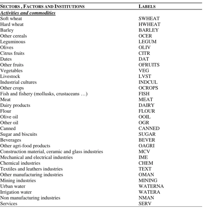
The micro SAM distinguishes 33 production sectors, including 23 agricultural and food activities with 10 urban industries and services; five types of labor namely, family agricultural workers, skilled and unskilled agricultural workers and skilled and unskilled nonagricultural workers; four types of land namely, annual irrigated and non irrigated land and perennial irrigated and non irrigated land; capital; and natural resources. Institutions include rural and urban households, companies, government and foreign trading partners (EU and ROW). This SAM provides a consistent set of relationships showing intermediate, final demand, value added and foreign transactions. The sectors, factors and institutions of the model are described in Table A5 in the appendix I along with their label.
The modeling analysis in this work is static by nature. As our SAM contains data on only two representative household groups, rural and urban households, the poverty and distributional impact from any simulation in the model cannot be computed with enough precision. To overcome this shortcoming, the CGE model is complemented by a micro-simulation methodology using the traditional “top-down” approach. We measure the distributional and poverty effects of agricultural trade policy changes using the 2000 expenditures household survey for Tunisia. The survey includes a nationally representative sample of about 6,000 households and contains information on household’s characteristics, household consumption expenditures on food and a comprehensive range of non-food items such as schooling, health, transportation and recreation. The sample is clustered and stratified by region and urban/rural areas.
As is common in most MENA countries, the survey does not include information on household’s income which is therefore approximated by expenditures. The “top-down” micro-simulation allows then to capture mainly the effects of consumption prices variations on individuals’ expenditures (income), poverty and inequality.23
.
5. Main Estimation Results
The ambition of our empirical investigation is to incorporate econometric evidence of the trade-productivity linkages into the CGE model to examine the impact of agricultural trade liberalization on poverty an inequality taking account of the farming productivity gains channel and the relationship between labor productivity and rigidities in the labor market.
23 For more details about the drawbacks of the “top-down” microsimulation method see Bourguignon et al.
We start by estimating the econometric model in section 2, and then incorporate the parameter estimates in the CGE model to investigate the inequality and poverty outcomes under different agricultural trade liberalization scenarios.
5.1 The econometric estimations
This empirical application involves basically a three-step analysis. First, the latent class model of equation (2) is estimated using maximum likelihood via the EM algorithm24. Second, efficiency and productivity levels and growth are computed for each country. Third, the technology gap among the different countries is measured, and the determinants of agricultural productivity growth are investigated focusing on the role of international trade. In each country, we carried out estimations at different levels of aggregation, both for each agricultural commodity group and for the whole agricultural sector. The results of estimating the input elasticities of the production frontier are reported in Table A3 in the appendix.25 The results show relatively important differences of the estimated factor elasticities among classes and seem to support the presence of technological differences across the countries. The input elasticities are globally positive and significant at the 10% level. Water and cropland have globally the largest elasticity, indicating that the increase of Mediterranean agricultural production depends mainly on these inputs. The estimated technology frontiers provide a measure of technical change. A positive sign on the time trend variable reflects technical progress. Significant shifts in the production frontier over time were found in the pooled and specific commodity models, indicating gains in technical change for the selected countries.
The determinants of agricultural production efficiency among the selected countries proved significant. International trade, educational attainment, land quality, agricultural research effort and institutional factors appear to contribute to enhancing efficient input use. As expected, the unequal distribution of agricultural land and to a lesser extent land fragmentation have significant adverse effects on efficient resource use.
The investigation of the estimation results of the latent class probability functions shows that the coefficients are globally significant, indicating that the variables included in the class probabilities provide useful information in classifying the sample. The sign of the parameters estimates indicate whether the separating variable increases the probability of assigning a
24 The estimation procedure was programmed in Stata 9.2.
25 In the interest of space limitation we describe the results using pooled data. Estimates for specific crops are
country into the corresponding class or not. For example, increasing total applied fertilizers increases the probability of a country to belong to class three.
The average efficiency scores and TFP changes, estimated using equations (6) and (7) respectively, are reported in Table A4 in the appendix. The results show productivity increases in the Mediterranean agricultural sector, on average, with SMC registering relatively better average rates of productivity gain than EU countries. On average, over the period under consideration, EU countries exhibited better efficiency levels than SMC.
Variation of agricultural performance across countries opens the possibility of investigating the factors contributing to productivity improvement and facilitating the catching up process between high-performing and low-performing countries. Two of the key concerns here are the relevance of international trade as a channel for technology spillovers and the importance of human capital for absorbing foreign knowledge and driving rates of productivity growth. To tackle this issue, we first measure the technology gap ratio (GAP), defined in section 2, using the metafrontier approach, and then estimate the model in equation (1) that links agricultural productivity growth to technology gap, international trade, and human capital using the nonlinear least squares approach.
The estimation of this model poses several challenges relating to unobserved heterogeneity, potential endogeneity, and measurement error. The computational difficulties of the nonlinear fixed effect models preclude the introduction of individual specific effects to control for the differences between the countries. We add a set of institutional factors, including investment in research and development, institutional quality and average agricultural holdings, to the baseline specification. This strategy enables us to control for heterogeneity in certain observed variables and to check the robustness of the results.
Another econometric concern is that measurement error and endogeneity of some explanatory variables, such as technology gap, could lead to bias in the estimated coefficients. On way of dealing with this problem is to regress the technology gap against the lagged gap and use the predicted value as an alternative to the technology gap in the model.
Table 2 reports the estimation results considering the two proxies of international trade, namely the ratio of agricultural exports plus imports to GDP (column 1), and agricultural trade barriers (column 2).
TABLE 2.IMPACT OF INTERNATIONAL TRADE ON AGRICULTURAL TFP GROWTH
TRADE VOLUMES TRADE BARRIERS
International trade*Human capital*(1-GAP) (α2) αop αH R&D Average holdings Control of corruption Government effectiveness Political stability 0.17* 0.34*** 0.35*** 0.024** 0.0038* 0.0003* 0.0004* 0.0003* -0.13*** -0.14*** -0.14** 0.029** 0.0022* 0.0002 0.0003* 0.0002* N. of observations R² adjusted 1260 0.62 1260 0.53
Notes: *, ** and *** denote statistical significance at the 10%, 5% and 1% levels respectively.
Regardless of the international trade measure, the results lend strong support to the positive effect of trade openness on agricultural productivity growth. Across the regressions, TFP growth rate increases with higher trade shares and decreases with more trade barriers. These estimates provide interesting insights into the agricultural productivity dynamics. The interaction term highlights the role of international trade in promoting technology transfer and point to the importance of education in facilitating the assimilation of foreign improvement of technology. The findings suggest that countries lying behind the frontier enjoy greater potential for TFP growth through the speed of technology transfer.
The linear effect of human capital on TFP provides also some support to the role of educational attainment in enhancing domestic innovation in agriculture.
There are also interesting results regarding the effect of the control variables on agricultural productivity growth. The findings provide evidence on the positive contribution of agricultural research efforts and larger farm sizes to productivity improvement. Control of corruption, government effectiveness and political stability enter with positive and statistically significant coefficients, indicating a positive role of institutional quality in enhancing agricultural growth.
5.2 Simulation of trade policy reform
The analysis aims to investigate the inequality and poverty impacts of agricultural trade liberalization and to examine the additional poverty alleviation that could be expected from the trade induced agricultural productivity gains. Two sets of scenarios are considered and under each scenario we abstract from the productivity gains and then take these gains into account. In what follows, we report the results for these scenarios:
1. Scenario 1: Cutting tariffs on agricultural products and abstracting from the productivity link.
2. Scenario 2: Cutting tariffs on agricultural products and taking account of the productivity link.
3. Scenario 3: This scenario extends Scenario 1 to all products. 4. Scenario 4: This scenario extends Scenario 2 to all products.
The simulation analysis focuses only on selected key variables, the choice of which relies on the mechanisms through which agricultural trade liberalization affects economic performance, poverty and inequality. The simulation results are reported using the percentage deviation from the model’s base-line, and in the interest of space limitation, most of the results refer to agriculture and agri-food.26
5.2.1 Impacts on production, imports and exports.
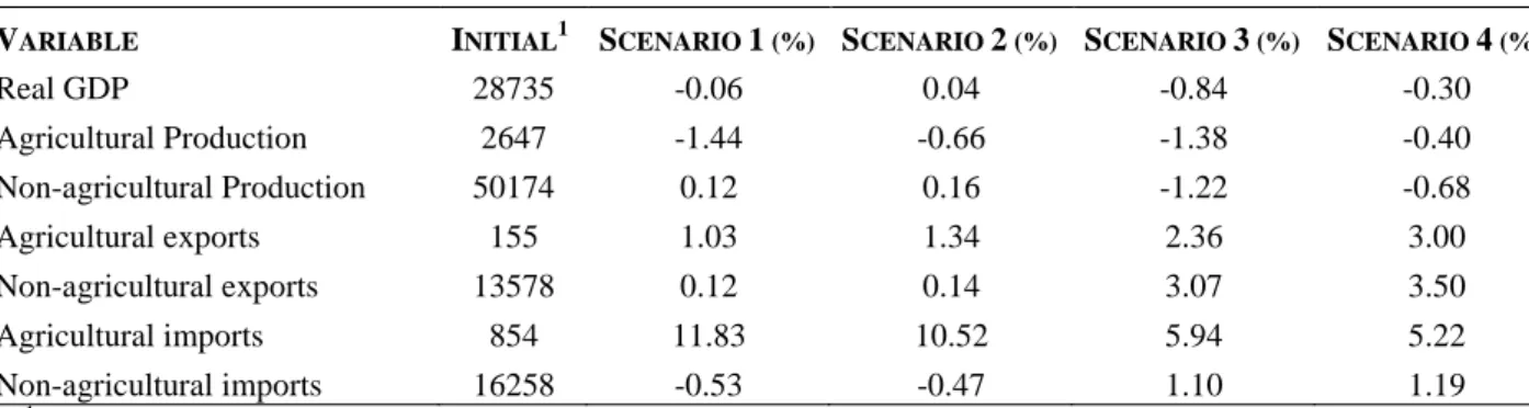
We begin by comparing the global impact of the four simulation scenarios on imports reported in Table 3 under Scenario 1. As expected agricultural trade openness exerts a significant positive effect on agricultural imports. The complete removal of tariffs on agricultural commodities induces a substantial reduction in the domestic prices of these commodities which, in turn, yields a substitution mechanism in favor of imported goods as these latter increase on average by 11.8 percent. Simultaneously and taking into account the degree of substitutability between imported and domestic agricultural products, the increased competitivity of imported commodities exerts a downward pressure on domestic prices that leads to a reduction in agricultural production of about 1.4 percent. This domestic prices decrease induces an increase of agricultural exports of 1 percent.27 With the domestic market becoming less attractive, farmers would choose to sell their products on the export market. We now examine what would happen if the trade-productivity linkages are incorporated in the model. As reported in the Scenario 2 of Table 3, using more efficient production techniques in the agricultural sector would in part counteract the trade’s negative effects of falling domestic prices on farming production. This is evident from the drop in agricultural production of only 0.7 percent compared to a drop of 1.4 percent in Scenario 1. Consequently, agricultural exports would increase more compared to the previous scenario (i.e. a rise of 1.3 percent rather than 1 percent) and imports would rise less (i.e. 10.5 percent instead of 11.8 percent).
26 Results on more variables and with different scenarios can be obtained from the authors upon request. 27 As is well known, the magnitude of this effect depends on the value of the elasticity of substitution in the CET
function. However, the basic mechanism remains almost unchanged even if we take more extreme values of the substitution elasticity.
We observe quite similar effects in the nonagricultural sectors. The findings reveal that with including the trade-productivity linkages the trade reforms will lead to a greater increase in exports and a lower increase in imports. However these effects are quite small.
Table 3 illustrates also the simulation results of full liberalization of agricultural and nonagricultural tariffs without and with endogenous productivity growth (scenarios 3 and 4, respectively). As shown in both scenarios, the elimination of all import tariffs results in a reduction in the domestic prices of these imports and induces a substitution in their favor. Although imports are boosted in all sectors, agricultural imports would increase the most (an increase of 5.9 percent compared to 1.1 percent for non-agricultural imports) as the initial tariff barriers are the highest in this sector. Taking account of the endogenous productivity effects would show a lower rise of agricultural imports (a rise of only 5.2 percent as opposed to a rise of 5.9 percent in the previous scenario) and nearly no change in nonagricultural imports.
In the trade liberalization scenarios without endogenous productivity effects, total production and GDP drop while exports increase in all sectors. This result can be traced primarily to the fall in domestic prices resulting from the removal of import tariffs. When the productivity effects are incorporated, we observe a lower decline in agricultural and nonagricultural production and a small increase in the real GDP under agricultural trade liberalization.
TABLE 3.MACROECONOMIC RESULTS
VARIABLE INITIAL1 SCENARIO 1 (%) SCENARIO 2 (%) SCENARIO 3 (%) SCENARIO 4 (%)
Real GDP 28735 -0.06 0.04 -0.84 -0.30 Agricultural Production 2647 -1.44 -0.66 -1.38 -0.40 Non-agricultural Production 50174 0.12 0.16 -1.22 -0.68 Agricultural exports 155 1.03 1.34 2.36 3.00 Non-agricultural exports 13578 0.12 0.14 3.07 3.50 Agricultural imports 854 11.83 10.52 5.94 5.22 Non-agricultural imports 16258 -0.53 -0.47 1.10 1.19
1 values in the base year are in Million TD
Table 4 illustrates the productivity gains as well as the imports and exports variations induced by the elimination of tariff on agricultural commodities (Scenario 2) and on all products (Scenario 4). The findings show important productivity gains in all agricultural productions. The sectors “Leguminous”, “Other fruits” and “Industrial cultures” seem to enjoy the most important productivity gains. These sectors are highly protected and the production and trade in these commodities are quite limited. Thus, the elimination of tariff barriers on these commodities appears to induce a substantial increase in their foreign trade enhancing the