HAL Id: hal-01238162
https://hal.inria.fr/hal-01238162
Submitted on 4 Dec 2015
HAL is a multi-disciplinary open access
archive for the deposit and dissemination of
sci-entific research documents, whether they are
pub-lished or not. The documents may come from
teaching and research institutions in France or
abroad, or from public or private research centers.
L’archive ouverte pluridisciplinaire HAL, est
destinée au dépôt et à la diffusion de documents
scientifiques de niveau recherche, publiés ou non,
émanant des établissements d’enseignement et de
recherche français ou étrangers, des laboratoires
publics ou privés.
Statistical Model Checking for SystemC Models
van Chan Ngo, Axel Legay, Jean Quilbeuf
To cite this version:
van Chan Ngo, Axel Legay, Jean Quilbeuf. Statistical Model Checking for SystemC Models. High
As-surance Systems Engineering Symposium, Jan 2016, Orlando, Florida, United States. �hal-01238162�
Statistical Model Checking for SystemC Models
Van Chan Ngo Axel Legay Jean Quilbeuf
INRIA, Campus Beaulieu, 35042 Rennes, France Email: {chan.ngo, axel.legay, jean.quilbeuf}@inria.fr
Abstract—Transaction-level modeling with SystemC has been very successful in describing the behavior of embedded systems by providing high-level executable models, in which many of them have an inherent probabilistic behavior, i.e., random data, unreliable components. It is crucial to evaluate the quantitative and qualitative analysis of the probability of the system prop-erties. Such analysis can be conducted by constructing a formal model of the system and using probabilistic model checking. However, this method is infeasible for large and complex systems due to the state space explosion. In this paper, we demonstrate the successful use of statistical model checking to carry out such analysis directly from large SystemC models and allows designers to express a wide range of useful properties.
Keywords-Runtime Verification, Probabilistic Assertion, Statis-tical Model Checking, Program Verification, SystemC
I. INTRODUCTION
Transaction-level modeling (TLM) with SystemC has been become increasingly prominent in describing the behavior of embedded systems [3], i.e., System-on-Chips (SoCs). It allows complex electronic components and software control units to be combined into a single model, enabling simulation of the whole system at once. In many cases, models include probabilistic characteristics, i.e, random data, reliability of the system’s components. It is crucial to evaluate the quantitive and qualitative analysis of the probability of the system’s properties. For instance, the reliability and availability of an embedded control system [14] that contains an input processor connected to groups of sensors, an output processor, connected to groups of actuators, and a main processor, that communi-cates with the I/O processors through a bus, can be modeled by a continuous-time Markov chain (CTMC) [25]. CTMC is a special case of a discrete-state stochastic process in which the probability distribution of the next state depends only on the current state. The analysis quantifies the probability or rate of all safety-related faults: How likely the system is available to meet a demand for service? What is the probability that the system repairs itself after a failure (e.g., that the system conforms to the existent and prominent standards such as the Safety Integrity Levels(SILs))?
In order to conduct such analysis, a general approach is modeling and analyzing a probabilistic model of the system (i.e, Markov chains, stochastic processes), in which the algo-rithm for computing the measures of properties depends on the class of systems being considered and the logic used for spec-ifying the properties. Many algorithms with the corresponding mature tools are based on model checking techniques that compute probability by a numerical approach [4], [21], [9]. For
a variety of probabilistic systems, the most popular modeling formalism is Markov chain or Markov decision processes, for which Probabilistic Model Checking (PMC) tools such as PRISM [10] and MRMC [13] can be used. PMC is widely used and has been successfully applied to the verification of a range of timed and probabilistic systems. One of the main challenges is the complexity of the algorithms in terms of execution time and memory space due to the size of the state space that tends to grow exponentially, also known as the state space explosion. As a result, the analysis is infeasible. In addition, these tools cannot work directly with the SystemC source code, meaning that a formal model of SystemC model needs to be provided. An alternative way to evaluate these systems is Statisti-cal Model Checking (SMC), a simulation-based approach. Simulation-based approaches produce an approximation of the value to be evaluated, based on a finite set of system’s executions. Clearly, comparing to the numerical approach, a simulation-based solution does not provide an exact answer. However, users can tune the statistical parameters such as the confidence interval and the confidence, according to the requirements. Simulation-based approaches do not construct all the reachable states of the model-under-verification (MUV), thus they require far less execution time and memory space than numerical approaches. For some real-life systems, they are the only one option [28] and have shown the advantages over other methods such as PMC [9], [12].
Our overall framework weaves the idea of statistical model checking to yield qualitative and quantitative analysis for prob-ability of a temporal property for SystemC models. The paper makes the following contributions: (i) we propose a framework to verify bounded temporal properties for SystemC models with both timed and probabilistic characteristics. The frame-work contains two main components: a monitor that observes a set of execution traces of the MUV and a statistical model checker implementing a set of hypothesis testing algorithms. We use techniques similar to the one proposed by Tabakov et al. [23] to automatically generate the monitor. The statistical model checker is implemented as a plugin of the checker Plasma Lab [2], in which the properties to be verified are expressed in Bounded Linear Temporal Logic (BLTL); (ii) we present a method that allows users to expose a rich set of user-code primitives in form of atomic propositions in BLTL. These propositions help users exposing the state of the SystemC simulation kernel and the full state of the SystemC source code model. In addition, users can define their own fine-grained time resolution that is used to reason on the semantics of the
logic expressing the properties rather the boundary of clock cycles in the SystemC simulation; and (iii) we demonstrate our approach through a running example, in which we showcase how our SMC-based verification framework works. We also illustrate the performance of the framework through some experiments.
II. BACKGROUND
A. SystemC and the Simulation Kernel
SystemC1 is a C++ library [6] providing primitives for
modeling hardware and software systems at the level of transactions. Every SystemC model can be compiled with a standard C++ compiler to produce an executable program called executable specification. This specification is used to simulate the system behavior with the provided event-driven simulator. A SystemC model is a hierarchical composition of modules (sc module). Modules are building blocks of SystemC design, they are like modules in Verilog [24], classes in C++. A module consists of an interface for communicating with other modules and a set of processes running concurrently to describe the functionality of the module. An interface contains ports (sc port), they are similar to the hardware pins. Modules are interconnected using either primitive channels (i.e., the signals, sc signal) or hierarchical channels via their ports. Channels are data containers that generate events in the simulation kernel whenever the contained data changes.
Processes are not hierarchical, so no process can call another process directly. A process is either a thread or a method. A thread process (sc thread) can suspend its execution by calling the library statement wait or any of its variants. When the execution is resumed, it will continue from that point. Threads run only once during the execution of the program and are not expected to terminate. On the other hand, a method process (sc method) cannot suspend its execution by calling wait and is expected to terminate. Thus, it only returns the control to the kernel when reaching the end of its body.
An event is an instance of the SystemC event class (sc event) whose occurrence triggers or resumes the execution of a process. All processes which are suspended by waiting for an event are resumed when this event occurs, we say that the event is notified. A module’s process can be sensitive to a list of events. For example, a process may suspend itself and wait for a value change of a specific signal. Then, only this event occurrence can resume the execution of the process. In general, a process can wait for an event, a combination of events, or for an amount of time to be resumed. In SystemC, integer values are used as discrete time model. The smallest quantum of time that can be represented is called time resolution meaning that any time value smaller than the time resolution will be rounded off. The available time resolutions are femtosecond, picosecond, nanosecond, microsecond, millisecond, and sec-ond. SystemC provides functions to set time resolution and de-clare a time object. The SystemC simulator is an event-driven simulation [1], [19]. It establishes a hierarchical network of
1IEEE Standard 1666-2005
finite number of parallel communicating processes which run under the supervision of the distinguished simulation kernel process. Only one process is dispatched by the scheduler to run at a time point, and the scheduler is non-preemptive, that is, the running process returns control to the kernel only when it finishes executing or explicitly suspends itself by calling wait. Like hardware modeling languages, the SystemC scheduler supports the notion of delta-cycles [16]. A delta-cycle lasts for an infinitesimal amount of time and is used to impose a partial order of simultaneous actions which interprets zero-delay semantics. Thus, the simulation time is not advanced when the scheduler processes a delta-cycle. During a delta-cycle, the scheduler executes actions in two phases: the evaluate and the update phases.
The simulation semantics of the SystemC scheduler is presented as follows: (1) Initialize. During the initialization, each process is executed once unless it is turned off by calling dont initialize(), or until a synchronization point (i.e., a wait) is reached. The order in which these processes are executed is unspecified; (2) Evaluate. The kernel starts a delta-cycle and runs all processes that are ready to run one at a time. In this same phase a process can be made ready to run by an event notification; (3) Update. Execute any pending calls to update() resulting from calls to request update() in the evaluate phase. Note that a primitive channel uses request update() to have the kernel call its update() function after the execution of processes; (4) Delta-cycle notification. The kernel enters the delta notification phase where notified events trigger their dependent processes. Note that immediate notifications may make new processes runnable during step (2). If so the kernel loops back to step (2) and starts another evaluation phase and a new delta-cycle. It does not advance simulation time; (5) Simulation-cycle notification. If there are no more runnable processes, the kernel advances simulation time to the earliest pending timed notification. All processes sensitive to this event are triggered, the kernel loops back to step (2) and starts a new delta-cycle. This process is finished when all processes have terminated or the specified simulation time is passed. B. Statistical Model Checking
We first recall the syntax and semantics of BLTL [22], an extension of Linear Temporal Logic (LTL) with time bounds on temporal operators. A formula ϕ is defined over a set of atomic propositions AP as in LTL by the grammar ϕ ::= true|f alse|p ∈ AP |ϕ1∧ ϕ2|¬ϕ|ϕ1 U≤T ϕ2, where the time
bound T is an amount of time or a number of states in the execution trace. The temporal modalities F (the “eventually”, sometimes in the future) and G (the “always”, from now on forever) can be derived from the “until” U as follows.
F≤T ϕ = true U≤T ϕ and G≤T ϕ = ¬F≤T ¬ϕ
The semantics of BLTL is defined w.r.t execution traces of a model. Let ω = (s0, t0)(s1, t1)...(sN −1, tN −1), N ∈ N be
an execution trace, ωk and ωk be the prefix and suffix of
ω respectively. We denote the fact that ω satisfies the BLTL formula ϕ by ω |= ϕ.
• ωk |= true and ωk 6|= f alse
• ωk |= p, p ∈ AP iff p ∈ L(sk), where L(sk) is the set
of atomic propositions which are true in state sk • ωk |= ϕ1∧ ϕ2 iff ωk|= ϕ1and ωk |= ϕ2 • ωk |= ¬ϕ iff ωk 6|= ϕ
• ωk |= ϕ1U≤T ϕ2iff there exists i ∈ N such that ωk+i|=
ϕ2, Σ0<j≤i(tk+j− tk+j−1) ≤ T , and for each 0 ≤ j <
i, ωk+j|= ϕ 1
Let M be the formal model of the MUV (i.e., a stochastic process) and ϕ be a property expressed as a BLTL for-mula. The statistical model checking [15] problem consists of answering the following questions: (i) Is the probability that M satisfies ϕ greater or equal to a threshold θ with a specific level of statistical confidence (qualitative analysis, written M |= P r≥θ(ϕ))? (ii) What is the probability that
M satisfies ϕ with a specific level of statistical confidence (quantitative analysis, written M |= P r(ϕ))? Many statistical model checker are implemented [27], [2] that have shown their advantages over other methods such as PMC on several case studies.
This is done by associating each execution trace of M with a discrete random Bernoulli variable Bi, in which the
outcome for Bi, denoted by bi, is 1 if the trace satisfies
ϕ and 0 otherwise. The predominant statistical method for verifying M |= P r≥θ(ϕ) is based on hypothesis testing.
Let p = P r(ϕ), to determine whether p ≥ θ, we test the hypothesis H0 : p ≥ p0 = θ + δ against the alternative
hypothesis H1 : p ≤ p1 = θ − δ based on the observations
of Bi. The size of indifference region is defined by p0− p1.
If we take acceptance of H0to mean acceptance of P r≥θ(ϕ)
as true and acceptance of H1 to mean rejection of P r≥θ(ϕ)
as false, then we can use acceptance sampling (e.g., Younes in [26] has proposed two solutions, called single sampling plan and sequential probability ratio test) to verify P r≥θ(ϕ). An
acceptance sampling test with strength (α, β) guarantees that H1is accepted with probability at most α when H0holds and
H0 is accepted with probability at most β when H1 holds,
called a Type-I error and Type-II error, respectively.
To answer the quantitative question, M |= P r(ϕ), an alternative statistical method, based on estimation instead of hypothesis testing, has been developed. For instance, the prob-ability estimations are based on results derived by Chernoff and Hoeffding bounds [11]. This approach uses n observations b1, ..., bn to compute an approximation of p: ˜p = n1Σ
n i=1bi.
The approximation satisifies that P r[|˜p − p| < δ] ≥ 1 − α. Based on the theorem of Hoeffding, the number of observa-tions which is determined from the absolute error δ and the confidence 1 − α is n = d2δ12log
2 αe.
Although SMC can only provide approximate results with a user-specified level of statistical confidence, it is compensated for by its better scalability and resource consumption. Since the models to be analyzed are often approximately known, an approximate result in the analysis of desired properties within specific bounds is quite acceptable. SMC has recently been applied in a wide range of research areas including software engineering (e.g., verification of critical embedded
systems) [9], system biology, or medical area [12]. III. A RUNNINGEXAMPLE
We will use a simple case study with a FIFO channel as a running example. This example illustrates how designers can create hierarchical channels that encapsulate both design structure and communication protocols. In the design, once a nanosecond the producer will write one character to the FIFO with probability p1, while the consumer will read one
character from the FIFO with probability p2. The FIFO which
is derived from sc channel encapsulates the communication protocol between the producer and the consumer.
The FIFO channel is designed to ensure that all data is reliably delivered despite the varying rates of production and consumption. The channel uses an event notification hanshake protocol for both the input and output. It uses a circular buffer implemented within a static array to store and retrieve the items within the FIFO. We assume that the sizes of the mes-sages and the FIFO buffer are fixed. Hence, it is obvious that the time required to transfer completely a message, or message latency, depends on the production and consumption rates, the FIFO buffer size, the message size, and the probabilities of successful writing and reading. The full implementation of the example can be obtained at the url2, in which the probabilities
of writing and reading are implemented with the Bernoulli distributions with probabilities p1 and p2 respectively from
GNU Scientific Library (GSL) [7].
The quantitative analysis under consideration is: “What is the probability that messages are transfered completely within T1 nanoseconds during T nanoseconds of operation?”. This
kind of analysis can, thus, be conducted in the early design steps. To formulate the underlying property more precisely, we have to take into account the agreement protocol between the producer and consumer, i.e., the simple protocol can be every message has special starting delimiter with the character ’&’ and ending delimiter with the character ’@’. Thus, the property can be translated in BLTL as follows:
ϕ = G≤T((c read = 0&0) → F≤T1(c read =
0@0))
where c read is the character read in the FIFO by the consumer. The input providing to the SMC checker is P r(ϕ). This property is expressed in terms of the characters read in the FIFO by the consumer, but the communication protocol between the producer and the consumer is abstracted at a very high level. It is an illustration of the types of properties that can be checked on TLM specifications. The verification of such a property at the transaction level can be connected to its counterpart at register-transfer level (RTL) in order to check the correctness of RTL implementations.
IV. SMCFORSYSTEMC MODELS
A. SystemC Model State
Temporal logic formulas are interpreted over execution traces and traditionally a trace has been defined as a sequence
of states in the execution of a model. Therefore before we can define an execution trace we need a precise definition of the state of a SystemC model simulation. We are inspired by the definition of system state in [23], which consists of the state of the simulation kernel and the state of the SystemC model. We consider the external libraries as black boxes, meaning that their states are not exposed.
The state of the kernel contains the information about the current phase of the simulation (i.e., delta-cycle notification, simulation-cycle simulation) and the SystemC events notified during the execution of the model. The state of the SystemC model is the full state of the C++ code of all modules in the model, which includes the values of the module attributes, the location of the program counter (i.e., a particular statement is reached during the execution of the model, the function calls), the call stack including the function execution, function parameters and return values, and the status of the module pro-cesses (i.e., suspended, runnable). We use V = {v0, ..., vn−1}
to denote the finite set of variables of primitive type (e.g, usual scalar or enumerated type in C/C++) whose value domain DX
represents the states of a SystemC model.
We consider here some examples about states of the simu-lation kernel and the SystemC model. Assume that a SystemC model has an event named e, then the model state can contain information such as the kernel is at the end of simulation-cycle notification phase and the event e is notified. Consider the running example again, a state can consist of the information about the characters received by the consumer, represented by the variable c read. It also contains the information about the location of the program counter right before and after a call of the function send() in the module Producer that are represented by two Boolean variables send start and send done, respectively, meaning that they hold the value true immediately before and after a call of the function send(). Another example, we consider a module that consists several statements at different locations in the source code, in which these statements contain the division operator “/” followed by zero or more spaces and the variable “a” (e.g., the statement y = (x + 1) / a). Then, a Boolean variable which holds the value true right before the execution of all such statements can be used as a part of the states.
We have discussed so far the state of a SystemC model execution. It remains to discuss how the semantics of the temporal operators is interpreted over the states in an execu-tion. That means how the states are sampled in order to make the transition from one state to another state. The following definition gives the concept of temporal resolution, in which the states are evaluated only at instances in which the temporal resolution holds. It allows the user to set granularity of time. Definition 1 (Temporal resolution): A temporal resolution Tris a finite set of Boolean expressions defined over V which
specifies when the set of variables V is evaluated.
Temporal resolution can be used to define a more fine-grained model of time than a coarse-grained one provided by a cycle-based simulation. We call the expressions in Tr temporal
events. Whenever a temporal event is satisfied or the temporal
event occurs, V is sampled. For example, in the producer and consumer model, assume that we want the satisfaction of the underlying BLTL ϕ to be checked whenever at the end of simulation-cycle notification or immediately after the event write eventis notified during a run of the model. Hence, we can define a temporal resolution as the following set Tr =
{end sc, we notif ied}, where end sc and we notified are Boolean expressions that have the value true whenever the kernel phase is at the end of the simulation-cycle notification and the event write event notified, respectively.
We denote the set of occurrences of temporal events from Tr along an execution of a SystemC model by Trs, called a
temporal resolution set. The value of a variable v ∈ V at an event occurrence ec∈ Trsis defined by a mapping ξvalv : Trs→
Dv, where Dvis the value domain of v. Hence, the state of the
SystemC model at ec is defined by a tuple (ξvalv0, ..., ξ vn−1
val ).
A mapping ξt: Trs→ T is called a time event that identifies
the simulation time at each occurrence of an event from the temporal resolution. Hence, the set of time points, called time tag, which corresponds to a temporal resolution set Trs =
{ec0, ..., ecN −1}, N ∈ N, is given as follows.
Definition 2 (Time tag): Given a temporal resolution set Ts
r, the time tag T corresponding to Trs is a finite or infinite
set of non-negative reals {t0, t1, ..., tN −1}, where ti+1− ti=
δti∈ R≥0, ti= ξt(eci). B. Model and Execution Trace
A SystemC model can be viewed as a hierarchical network of parallel communicating processes. Hence, the execution of a SystemC model is an alternation of the control between the model’s processes, the external libraries and the kernel process. The execution of the processes is supervised by the kernel process to concurrently update new values for the signals and variables w.r.t the cycle-based simulation. For example, given a set of runnable processes in a simulation-cycle, the kernel chooses one of them to execute first in a non-deterministic manner as described in the prior section.
Let V be the set of variables whose values represent the states of a SystemC model. The values of variables in V are determined by a given probability distribution (i.e., production from all probability distributions used in the model). Given a temporal resolution Tr and its
cor-responding temporal resolution set along an execution of the model Trs = {ec0, ..., ecN −1}, N ∈ N, the evaluation of V at the event occurrence eci is defined by the tuple (ξv0
val, ..., ξ vn−1
val ), or a state of the model at eci, denoted by V (eci) = (V (eci)(v0), V (eci)(v1), ..., V (eci)(vn−1)), where V (eci)(vk) = ξ
vk
val(eci) with k = 0, ..., n − 1 is the value of the variable vk at eci. We denote the set of all possible evaluations by VTs
r ⊆ DV, called the state space of the random variables in V . State changes are observed only at the moments of event occurrences. Hence, the operational semantics of a SystemC model is represented by a stochastic process {(V (eci), ξt(eci)), eci ∈ T
s
r}i∈N, taking values in
VTs
r × R≥0and indexed by the parameter eci, which are event occurrences in the temporal resolution set Ts
trace is a realization of the stochastic process is given as follows.
Definition 3 (Execution trace): An execution trace of a SystemC model corresponding to a temporal resolution set Ts
r = {ec0, ..., ecN −1}, N ∈ N is a sequence of
states and event occurrence times, denoted by ω =
(s0, t0)...(sN −1, tN −1), such that for each i ∈ 0, ..., N − 1,
si = V (eci) and ti= ξt(eci).
N is the length (finite or infinite) of the execution, also denoted by |ω|. Let V0 ⊆ V , the projection of ω on V0, denoted by
ω ↓V0, is an execution trace such that |ω ↓V0 | = |ω| and ∀v ∈ V0, ∀e
c∈ Trs, V0(ec)(v) = V (ec)(v).
C. Expressing Properties
Our approach allows users to refer to a rich set of atomic propositions AP which is defined over the set of variables V as previously mentioned. These propositions abstract the states of a SystemC model and evaluate to either true or false in such a state. The implementation provides a mechanism that allows users to declare V in order to define the set of propositions AP without requiring users to write the monitoring code or to write aspect-oriented programming advices manually.
Users declare these variables via a high-level language in a configuration file as the input of our tool. For instance, referring to the producer and consumer model, the declara-tion locadeclara-tion send start “%Producer::send()”:call declares a Boolean variable send start that holds the value true imme-diately before the execution of the model reaches a call site of the function send() in the module Producer. The characters received by the consumer which is represented by the variable c read can be declared as attribute pnt con→c int c read, where pnt con is a pointer to the Consumer object and c int is an attribute of the Consumer module representing the received character. The detailed syntax can be found in the tool manual3.
AP are predicates defined over the set of variables V . Using these predicates, users can define temporal properties related to the states of the kernel and the SystemC model. Recall the considered property of the running example, the predicates which are defined over the variable c read are c read =0&0 and c read =0@0. Another example, assume that we want to answer the following question: “Over a period of T time units, is the probability that the number of elements in the FIFO buffer in betweenn1 andn2 is greater or equal toθ with the
confidenceα?”. The predicates need to be defined in order to construct the underlying BLTL formula are n1 ≤ nelements
and nelements ≤ n2, where nelements is an integer variable
that represents the current number of elements in the FIFO buffer (it captures the value of the num elements attribute in the Fifo module). Then, the property can be translated in BLTL with the operator “always” as follows. The input which is given to the checker is P r≥θ(ϕ) along with the confidence α.
ϕ = G≤T((n1≤ nelements) & (nelements≤ n2))
3https://project.inria.fr/plasma-lab/documentation/tutorial/mag manual/
V. IMPLEMENTATION
A. MAG and SystemC Plugin
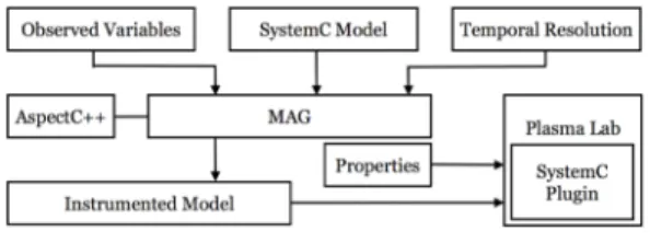
Fig. 1 shows our SMC-based verification tool implementa-tion that contains two main components: a monitor and aspect-advice generator (MAG) and a statistical model checker (SystemC Plugin). In principle, the full state can be observed during the simulation of the model. In practice, however, users define a set of variables of interest, according to the properties that the users want to verify, called observed variables, and only these variables appear in the states of an execution trace. Given a SystemC model, we use Vobs ⊆ V to denote
Fig. 1: The framework’s flow
the set of observed variables, to expose the states of the SystemC model. Then, the observed execution traces of the model are the projections of the execution traces on Vobs,
meaning that for every execution trace ω, the corresponding observed execution trace is ω ↓Vobs. In the following, when we mention execution traces, we mean observed execution traces. The implementation of MAG allows users to define a set of observed variables that is used with a temporal resolution to generate a monitor. The implementation based on the techniques in [23], in which a monitor and a file containing aspects are generated in order to automatically instrument the SystemC model with the help of AspectC++ [5] and establish a communication between the generated monitor and the instrumented model. The monitor evaluates the set of observed variables at every time point at which an event of the temporal resolution occurs during the SystemC model simulation to produce a new state. For example, the variable c read which observes the character received by the consumer (the private attribute c int in the module Consumer) at the end of simulation-cycle notification, is implemented by generating a monitor and instrumenting the module Consumer to establish a communication between them as follows. The module Con-sumeris instrumented with AspectC++, in this case, such that the monitor is its friend class, so the monitor can access the private attributes of Consumer. The monitor defines a callback function being called immediately at the end of simulation-cycle notification, and a pointer pointing to an instance of Consumer. The execution of the callback function consists of getting the current value of the received character by the consumer, assigning this character to c read, and executing the monitor for one step (i.e., creating a new state and reporting it to the Plasma plugin). If temporal resolutions involving kernel simulation phases or event notifications are defined, the calling mechanism of the callback function is realized
by modifiying the kernel (i.e., at the end of simulation-cycle segment code, a call to the callback function is added).
The statistical model checker is implemented as a plugin of Plasma Lab [2] that establishes a communication, in which the generated monitor transmits execution traces of the MUV. In the current version, the communication is done via the standard input and output. When a new state is requested, the monitor reports the current state (the values of variables in Vobs) to the plugin. The length of traces depends on the
satisfaction of the formula to be verified, which is finite because the temporal operators are bounded. Similarly, the required number of execution traces depends on the hypothesis testing algorithms in use (e.g., sequential hypothesis testing or 2-sided Chernoff bound). The full implementation can be downloaded on the website of Plasma Lab4.
B. Running Verification
Running the verification tool consists of two steps as follows. First, users define a set of observed variables and a temporal resolution in a configuration file, as well as other necessary information as an input for MAG to generate a monitor and an aspect-advices file. AspectC++ is then used to instrument automatically the model. The instrumented model and the generated monitor are compiled and linked together with the SystemC kernel into an executable model in order to make a set of execution traces. Referring to the running example, users will define the set of observed variables Vobs=
{c read, nelements, end sc}, where c read is the character
read in the FIFO, nelementsis the number of characters in the
FIFO buffer, and end sc is true whenever the kernel phase is at the end of the simulation-cycle notification phase. The tem-poral resolution will be defined as Tr = {end sc}, meaning
that a new state in execution traces is produced whenever the simulation kernel is at the end of simulation-cycle notification phase or every one nanosecond in the example since the time unit is one nanosecond. The full configuration file is included in the source code of the example.
In the second step, the plugin is used to verify the properties of interest. The satisfaction checking of the properties is brought out based on the set of execution traces obtained by executing the instrumented SystemC model and can be done by several hypothesis testing algorithms provided by Plasma Lab.
VI. CASESTUDIES
We report the experimental results for the running example and also demonstrate the use of our verification tool to analyze the dependability of a large embedded control system. The number of components in this system makes numerical approaches such as PMC infeasible. In both case studies, we used the 2-sided Chernoff bound algorithm with the absolute error δ = 0.02 and the confidence 1 − α = 0.98. The experiments were run on a machine with an Intel Core i7 2.67 GHz processor and 4GB RAM under the Linux OS with
4https://project.inria.fr/plasma-lab/download/plugins/
SystemC 2.3.0, in which the checking of the properties in the running example took from less than one minute to several minutes. The analysis of the embedded and control system case study takes almost 2 hours, in which 90 properties were verified.
A. Producer and Consumer
Let us go back to the running example in Section III, recall that we want to compute the probability that the following property ϕ satisfies every 1 nanosecond, with the absolute error 0.02 and the level of confidence 0.98. In this verifi-cation, both the FIFO buffer size and message size are 10 characters including the starting and ending delimiters, and the production and consumption rates are 1 nanosecond. First, we check this property with the various values of p1 and
p2. The results are given in Table I with T = 5000 and
T1 = 25 nanoseconds. It is trivial that the probability that
the message latency is smaller than T1 time increases when
p1 and p2 increase. That means that, in general, the latency
is shorter when the either the probability that the producer successfully writes to the FIFO increases, or the probability that the consumer successfully reads from the FIFO increases. Second, we compute the probability that a message is sent
p1\p2 0.3 0.6 0.9
0.6 0 0.0194 0.0720
0.9 0 0.0835 1
TABLE I: The probability that the message latency is smaller than 25 in the first 5000 nanoseconds of operation
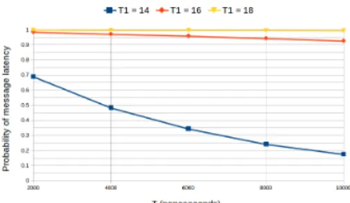
Fig. 2: The probability that the message latency is smaller than T1 in the first T nanoseconds of operation
completely (or the message latency) from the producer to the consumer within T1 time over a period of T time of
operation, in which the probabilities p1 and p2 are fixed at
0.9. Fig. 2 shows this probability with different values of T1
over T = 10000 nanoseconds. It is observed that the message latency is almost smaller than 18 nanoseconds.
B. An Embedded Control System
This case study is closely based on the one presented in [20], [14] but contains much more components. The system consists of an input processor (I) connected to 50 groups of
3 sensors, an output processor (O), connected to 30 groups of 2 actuators, and a main processor (M ), that communicates with I and O through a bus. At every cycle, 1 minute, the main processor polls data from the input processor that reads and processes data from the sensor groups. Based on this data, the main processor constructs commands to be passed to the output processor for controlling the actuator groups.
The reliability of the system is affected by the failures of the sensors, actuators, and processors. The probability of bus failure is negligible, hence we do not consider it. The sensors and actuators are used in 37 − of − 50 and 27 − of − 30 modular redundancies, respectively. That means if at least 37 sensor groups are functional (a sensor group is functional if at least 2 of the 3 sensors are functional), the system has enough information to function properly. Otherwise, the main processor is reported to shut the system down. In the same way, the system requires at least 27 functional actuator groups to function properly (a actuator group is functional if at least 1 of the 2 actuators is functional). Transient and permanent faults can occur in processors I or O and prevent the main processor (M ) to read data from I or send commands to O. In that case, M skips the current cycle. If the number of continuously skipped cycles exceeds the limit K, the processor M shuts the system down. When a transient fault occurs in a processor, rebooting the processor repairs the fault. Lastly, if the main processor fails, the system is automatically shut down. The mean times to failure for the sensors, the actuators, and the processors are 1 month, 2 months and 1 year, respectively. The mean time to transient failure is 1 day and I/O processors take 30 seconds, 1 time unit, to reboot.
The reliability of the system is modeled as a CTMC [18], [25] that is realized in SystemC, in which a sensor group has 4 states (0, 1, 2, 3, the number of working sensors), 3 states (0, 1, 2, the number of working actuators) for an ac-tuator group, 2 states for the main processor (0: failure, 1: functional), and 3 states for I/O processors (0: failure, 1: transient failure, 2: functional). A state of the CTMC is represented as a tuple of the component’s states, and the mean times to failure define the delay before which a transition between states is enabled. The delay is sampled from a negative exponential distribution with parameter equal to the corresponding mean time to failure. Hence, the model has about 2155 states comparing to the model in [14] with about 210states, that makes the PMC technique is unfeasible.
That means the state explosion likely occurs, even with some abstraction, i.e., symbolic model checking is applied. The full implementation of the SystemC code and experiments of this case study can be obtained at the website of our tool5. We
define four types of failures: f ailure1 is the failure of the
sensors, f ailure2 is the failure of the actuators, f ailure3 is
the failure of the I/O processors and f ailure4 is the failure
of the main processor. For example, f ailure1 is defined by
number sensors < 37) ∧ (proci status = 2). It specifies that the number of working sensor groups has decreased
5https://project.inria.fr/plasma-lab/embedded-control-system/
below 37 and the input processor is functional, so that it can report the failure to the main processor. We define f ailure2,
f ailure3, and f ailure4 in a similar way.
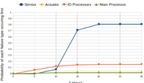
In our analysis which is based on the one in [14] with K = 4, in which the properties are checked every 1 time unit. First, we try to determine which kind of component is more likely to cause the failure of the system, meaning that we determine the probability that a failure related to a given component occurs before any other failures. The atomic proposition shutdown = W4
i=1f ailurei indicates that the
system has shut down because one of the failures has occurred, and the BLTL formula ¬shutdown U≤T f ailurei states that
the failure i occurs within T time units and no other failures have occurred before the failure i occurs. Fig. 3 shows the probability that each kind of failure occurs first over a period of 30 days of operation. It is obvious that the sensors are likelier to cause a system shutdown. At T = 20 days, it seems that we reached a stationary distribution indicating for each kind of component the probability that it is responsible for the failure of the system.
Fig. 3: The probability that each of the 4 failure types is the cause of system shutdown in the first T time of operation
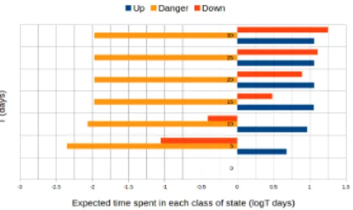
For the second part of our analysis, we divide the states of system into three classes: “up”, where every component is functional, “danger”, where a failure has occurred but the system has not yet shut down (e.g., the I/O processors have just had a transient failure but they have rebooted in time), and “shutdown”, where the system has shut down [14]. We aim to compute the expected time spent in each class of states by the system over a period of T time units. To this end, we add in the model, for each class of state c, a random variable reward c that measures the time spent in the class c. In our tool, the formula X≤T reward c returns the mean value of
reward c after T time of execution. The results are plotted in Fig. 4. From T = 20 days, it seems that the amounts of time spent in the “up” and “danger” states are converged at 101.063= 11.57 days and 10−1.967= 0.01 days, respectively.
VII. RELATEDWORK ANDCONCLUSION
There has been a lot of work on the formalization of SystemC [8], [17]. The goal is to extract a formal model from a SystemC program, so that tools like model-checkers can be applied. However, all these formalizations consider semantics
Fig. 4: The expected amount of time spent in each of the states: “up”, “danger” and “shutdown”
of SystemC and its simulator in some form of global model, and they also suffer from the state space explosion when dealing with industrial and large systems.
In [29], Zuliani et al. extended the standard SMC algorithm for verifying Stateflow/Simulink models of a fuel control system featuring fault-tolerance and hybrid behavior, in which properties under verification are expressed in BLTL. The ex-tension is based on Bayesian interval estimation and Bayesian sequential hypothesis testing. This technique is scalable for larger Stateflow/Simulink models because verification is fast in most cases and the Bayesian estimation is orders of mag-nitudes faster than previous estimation-based model checking algorithms.
Tabakov et al. [23] proposed a framework for monitoring temporal SystemC properties. This framework allows users to express the properties to verify by fully exposing the semantics of the simulator as well as the user-code. They extend LTL by providing some extra primitives for stating the atomic propo-sitions and let users define a much finer temporal resolution. Their implementation consists of a modified simulation kernel, and a tool to automatically generate the monitors and aspect advices for instrumenting SystemC programs automatically.
This paper presents the first attempt to verify non-trivial temporal properties of a SystemC model with statistical model checking techniques. The framework contains two main com-ponents: a generator that automatically generates a monitor and instruments the MUV based on the properties to be verified, and a statistical model checker implementing a set of hypothesis testing algorithms. In comparison to the probabilis-tic model checking, our approach allows users to handle large industrial systems, expose a rich set of user-code primitives in form of atomic propositions in BLTL, and work directly with SystemC models. For instance, our verification framework is used to analyze the dependability of large industrial computer-based control systems as shown in the case study.
Currently, we consider an external library as a “black box”, meaning that we do not consider the states of external libraries. Thus, arguments passed to a function in an external library cannot be monitored. For future work, we would like to allow users to monitor the states of the external libraries. We also plan to apply statistical model checking to verify temporal properties of SystemC-AMS (Analog/Mixed-Signal).
REFERENCES
[1] Accellera. http://www.accellera.org/downloads/standards/systemc. [2] B. Boyer, K. Corre, A. Legay, and S. Sedwards. Plasma lab: A flexible,
distributable statistical model checking library. In QEST’13, 2013. [3] H. Chang, L. Cooke, M. Hunt, G. Martin, A. McNelly, and L. Todd.
Surviving the soc revolution: A guide to platform-based design. In Norwell, USA, 1999.
[4] F. Ciesinski and M. Grober. On probabilistic computation tree logic. In Validation of Stochastic Systems, 2004.
[5] A. Gal, W. Schroder-Preikschat, and O. Spinczyk. Aspectc++: Language proposal and prototype implementation. In OOPSLA’01, 2001. [6] T. Grotker, S. Liao, G. Martin, and S. Swan. System Design with
SystemC. Kluwer Academic Publishers, Norwell, USA, 2002. [7] GSL. http://www.gnu.org/software/gsl/.
[8] P. Herber, J. Fellmuth, and S. Glesner. Model checking systemc designs using timed automata. In CODES/ISSS’08, 2008.
[9] H. Hermanns, B. Watcher, and L. Zhang. Probabilistic cegar. In CAV’08. LNCS, Springer, 2008.
[10] A. Hinton, M. Kwiatkowska, G. Norman, and D. Parker. Prism: A tool for automatic verification of probabilistic systems. In TACAS’06. LNCS, Springer, 2006.
[11] W. Hoeffding. Probability inequalities for sums of bounded random variables. In American Statistical Association, 1963.
[12] S. Jha, E. Clarke, C. Langmead, A. Legay, A. Platzer, and P. Zuliani. A bayesian approach to model checking biological systems. In CMSB’09. LNCS, Springer, 2009.
[13] J. Katoen, E. Hahn, H. Hermanns, D. Jansen, and I. Zapreev. The ins and outs of the probabilistic model checker mrmc. In QEST’09, 2009. [14] M. Kwiatkowska, G. Norman, and D. Parker. Controller dependability
analysis by probabilistic model checking. In Control Engineering Practice. Elsevier, 2007.
[15] A. Legay, B. Delahaye, and S. Bensalem. Statistical model checking: An overview. In RV’10, 2010.
[16] R. Lipsett, C. Schaefer, and C. Ussery. VHDL: Hardware description and design. Kluwer Academic Publishers, 1993.
[17] F. Maraninchi, M. Moy, C. Helmstetter, J. Cornet, C. Traulsen, and L. Maillet-Contoz. Systemc/tlm semantics for heterogeneous socs validation. In NEWCAS/TAISA’08, 2008.
[18] M. A. Marsan and M. Gerla. Markov models for multiple bus multiprocessor systems. In IEEE Transactions on Computer, 1982. [19] W. Mueller, J. Ruf, D. Hoffmann, J. Gerlach, T. Kropf, and W.
Rosen-stiehl. The simulation semantics of systemc. In DATE 2001, 2001. [20] J. Muppala, G. Ciardo, and K. Trivedi. Stochastic reward nets for
reliability prediction. In CRMS’94, 1994.
[21] J. Rutten, M. Kwiatkowska, G. Norman, and D. Parker. Mathematical techniques for analyzing concurrent and probabilistic systems. In CRM Monograph Series, 2004.
[22] K. Sen, M. Viswanathan, and G. Agha. On statistical model checking of stochastic systems. In CAV’05, 2004.
[23] D. Tabakov and M. Vardi. Monitoring temporal systemc properties. In Formal Methods and Models for Codesign, 2010.
[24] D. Thomas and P. Moorby. The verilog hardware description language. In Springer. ISBN 0-3878-4930-0, 2008.
[25] K. S. Trivedi. Probability and statistics with reliability, queueing, and computer science applications. In Englewood Cliffs, 1982.
[26] H. Younes. Verification and planning for stochastic processes with asynchronous events. In PhD Thesis, Carnegie Mellon, 2005. [27] H. Younes. Ymer: A statistical model checker. In CAV’05, 2005. [28] H. Younes, M. Kwiatkowska, G. Norman, and D. Parker. Numerical vs
statistical probabilistic model checking. In STTT’06, 2006.
[29] P. Zuliani, A. Platzer, and E. M.Clarke. Bayesian statistical model checking with application to simulink/stateflow verification. In Formal Methods in System Design, 2013.