Journal of Fundamental and Applied Sciences is licensed under a Creative Commons Attribution-NonCommercial 4.0 International License. Libraries Resource Directory. We are listed under Research Associations category.
A NEW ANALYTICAL MODELING METHOD FOR PHOTOVOLTAIC SOLAR CELLS BASED ON DERIVATIVE POWER FUNCTION
R. Zieba Falama1,2,*, A. Dadjé1,3, N. Djongyang1 and S.Y. Doka4
1
Department of Renewable Energy, The Higher Institute of the Sahel, University of Maroua, P.O Box 46 Maroua, Cameroon
2
Institute of Geological and Mining Research, P.O. Box 4110 Yaoundé, Cameroon
3
School of Geology and Mining Engineering, University of Ngaoundéré, P.O Box 454 Ngaoundere, Cameroon
4
Department of Physics, Faculty of Science, University of Ngaoundéré, P.O Box 454 Ngaoundere, Cameroon
Received: 25 Jaunary 2016 / Accepted: 25 April 2016 / Published online: 01 May 2016
ABSTRACT
This paper presents a simple method of optimizing the photovoltaic (PV) generator based on the one diode electrical model. The method consists in solving a second degree equation representing the derivative of the power function. The maximum current and voltage are determined, and the maximum power is deduced. Two popular types of photovoltaic panels constructed with different materials have been considered for the test: the multi-crystalline silicon (Shell S75), and the mono-crystalline silicon (Shell SP70). For various environmental conditions, a comparative study is done between the simulated results and the product manufacturer data. The obtained results prove the efficiency of the proposed method.
Keywords: model; photovoltaic generator; power function; optimizing, maximum power.
Author Correspondence, e-mail: [email protected]
doi: http://dx.doi.org/10.4314/jfas.v8i2.17
ISSN 1112-9867
1. INTRODUCTION
Solar energy applications have been increasing gradually throughout the world. This is due to the decrease in the cost of PV panels with the increasing demand, and the increase in duration of use (lifetime). Photovoltaic is very competitive in areas far from the conventional electricity network. However, its exploitation requires a conception and implantation of a production system which also require a good sizing in order to avoid losses or lack of energy.
The evaluation of the maximum power produced by a PV generator is very important to size a PV system. Several models have been developed to determine the maximum power produced by a PV generator. In general, two main approaches are found in the literature [1, 2].
Nomenclature
I : Cell current (A)
V : Cell Voltage (V)
Iph : Light current (A)
ID : Diode current (A)
Ish : Shunt current (A)
Io : Saturation current of the diode (A)
Io,ref : The reverse saturation current (A)
Isc : Short circuit current (A)
Voc : Open circuit voltage (V)
α :
Temperature coefficient of short-circuit current (A/K)
Tc : Cell Temperature (Kelvin)
Tr : Cell Temperature at reference condition (25°C or 298 K)
Imp : Current at peak power point in reference condition (A)
Vmp : Voltage at peak power in reference condition (V)
G : Irradiance (W/m²)
Gr : Irradiance at reference condition (W/m²)
n : Ideality factor of the diode
N : Number of cells in series
k : Boltzmann constant (1.38×10⁻²³
J/K)
q : Electron charge (1.6×10⁻¹⁹
coulomb)
Rs : Series resistance of generator (Ω)
Rsh : Shunt resistance (Ω)
Eg : Gap Energy (for the silicon Eg =1.12 eV)
The first approach requires taking some measurements once the PV generator is installed. This is the case of Sandia and Cenerg models [3]. The second approach consists in using solely the data provided by the manufacturer; e.g. of Borowy and Salameh’s model [4] and the model of Jones et al [5]. Modeling a PV generator needs to evaluate the different parameters of the module. The number of theses parameters varies with the type of module. In this study a one diode PV generator with five parameters is used.
Generally, the five parameters determination of a one diode PV generator is difficult due to the exponential equation of the diode p-n junction. The commonly used methods to determine these parameters are the analytical method, but recently novel techniques using computational intelligence algorithms have been carried out such as cuckoo search (CS) [6], pattern search (PS) [7], Chaos Particle Swarm Optimization (CPSO) [8], genetic algorithm (GA) [9], fuzzy logic (FL) [10], artificial neural network (ANN) [11, 12]. The analytical method based on datasheet is used in this work.
In ref. [2], a data-based approach has been presented to estimate the maximum power of the PV generator. An iterative method was used to solve the nonlinear equation of the maximum current, obtained by the derivative of power with respect to voltage.
used the derivative of power with respect to current and limit development, in order to estimate the maximum power of the photovoltaic generator.
To prove the efficiency of the proposed model, a comparison is doing with the data provided by the manufacturers for two types of photovoltaic panels.
2. PRESENTATION OF THE METHOD 2.1. Modeling of the photovoltaic generator
In the literature, two main electric photovoltaic generator models exist; namely the one and two diodes models, with three or several parameters. In this work, a one diode photovoltaic module with five parameters whose equivalent diagram is presented in figure 1 is studied. The
five parameters here are: Iph, Rs, Rsh, I0, and n.
Fig.1. Electrical model of a PV generator with five parameters [1,4]
The current produced by the generator is obtained from Kirchhoff’s laws as follows:
ph D
I =I +I (1)
The diode current can be obtained through Shockley equation as follows [13]:
(
)
exp s 1 D o c q V R I I I nNkT + = − (2)While the shunt current is given by the relation:
s sh sh V R I I R + = (3) Replacing (2) and (3) into (1) give the photovoltaic current as:
(
)
exp s 1 s ph o c sh q V R I V R I I I I nNkT R + + = − − − (4)In practice shunt resistance has a high values, therefore the term S 0 sh V R I R + → [14, 15], so:
(
)
exp s 1 ph o c q V R I I I I nNkT + = − − (5)2.1.1. Determination of the PV generator parameters 2.1.1.1. Evaluation of Iph
The light current Iph depends on both irradiance and temperature. It is given by [13, 15]:
(
)
ph sc c r r G I I T T G α = + − (6) 2.1.1.2. Evaluation of IoThe reverse saturation current depending of cells temperature is given as follows [13, 15]:
3 , 1 1 .exp g r c c o o n r qE T T T I I T nk − = (7)
At the open circuit voltage, I=0, V=Voc and Iph=Isc:
, 0 exp oc 1 sc o n c qV I I nNkT = − − (8)
So the nominal saturation current is obtained through:
, exp 1 sc o n oc c I I qV nNkT = − (9)
By replacing the eq. (9) into eq. (7) one gets:
3 1 1 .exp exp 1 g r c sc c o r oc c qE T T I T I T nk qV nNkT − = − (10) 2.1.1.3. Evaluation of Rs
the series resistance is evaluated as follows: oc s V V dV R dI = = − (11)
Considering the asymptotic behavior of the I-V curve at short-and open-circuit conditions [21],
(11) can be calculated as:
oc mp s s mp V V R N I − = (12) 2.1.1.4. Evaluation of n
At the short circuit point, I=Isc, V=0:
, , exp 1 s sc sc ph ref o ref r qR I I I I nNkT = − − (13)
At the maximum power point, I=Imp,V=Vmp:
(
)
, , exp 1 mp s mp mp ph ref o ref r q V R I I I I nNkT + = − − (14)The reverse saturation current Io for any diode is a very small quantity, on the order of 10-5 or
10-6 A [2]. This minimizes the impact of the exponential term in Eq. (13), so it is safe to assume
that the photocurrent equals the short-circuit current [22]. Another simplification [23] can be made regarding the first term in eqs. (8) and (14). In both cases, regardless of the system size, the exponential term is much greater than the first term. For this reason the first term can be neglected. Then, the equation system becomes:
, sc ph ref I ≈I (15) , 0 .exp oc sc o ref r qV I I nNkT = − (16)
(
)
, , exp mp s mp mp ph ref o ref r q V R I I I I nNkT + = − (17)Combining (16) and (17), the ideality factor is evaluated as follows:
(
)
ln mp s mp oc sc mp r sc q V R I V n I I NkT I + − = − (18)2.2. Maximum power point determination
By using the expression of the PV current defined by eq. (5), the voltage supplied by the generator is: ln 1 ph c s o I I nNkT V R I q I − = + − (19)
The electric power produced by the generator is given by: .
P=V I (20) By replacing (19) into (20) one obtain,
2 ln 1 ph c s o I I nNkT I P R I q I − = + − (21) From the function P = f (I), the extremum is obtained by the resolution of the equation
0 P V ∂ = ∂ i.e.
(
)
(
)
2 2 s ln 1 ph 2 s o ph . ln 1 ph o ph 0 o o I I I I R I C C R I I I C I I I I − − − + + + + + + + = (22)In the above equation (22), c
nNkT C
q
= (23)
The limit development near of I = 0, in one order for ln 1 ph
o I I I − + is given by: ln 1 ph ln 1 ph o o o ph I I I I I I I I − + = + − + (24)
By replacing equation (24) into equation (22), one can have:
(
)
(
)
(
)
2 2 s ln 1 ph 2 s o ph . ln 1 ph o ph o ph 0 o o ph o o ph CI I I I CI I R I C C R I I I C I I I I I I I I + − + − + + + + + + − = + + (25)By rearranging eq. (25), one can obtain the equation of the second degree (26) below:
(
)
(
)
2(
)
(
)
(
)
2 2 s o ph o ph ln 1 ph 2 2 s o ph . ln 1 ph o ph 0 o o I I C R I I I I I C C R I I I C I I I I + + − + + + + + + + + = (26)
To solve this equation of the second degree let’s put:
(
)
(
)
1 2 s o ph X = C+ R I +I (27)(
)
(
)
2 ln 1 2 2 ph o ph s o ph o I X I I C C R I I I = − + + + + + (28)(
)
2 3 ln 1 ph o ph o I X C I I I = + + (29)The eq. (26) could be rewritten as follows:
2
1. 2. 3 0
X I +X I+X = (30)
The resolution of eq. (30) permits to obtain the following solutions:
2 2 2 1 3 max 1 4 2 X X X X I X − ± − = (31) max max ln 1 max ph c s o I I nNkT V R I q I − = + − (32)
max max. max
P =V I (33) Imax, Vmax, and Pmax are respectivement the maximum current, the maximum voltage and the
maximum power.
Iph, Io, Rs, n and C are respectively given by equations (6), (10), (12), (18) and (23).
3. RESULTS AND DISCUSSION
The chosen points for the parameters determination under reference conditions are mainly: the
short-circuit current (0, ISC), the open-circuit voltage point (0, Voc), and the maximum power
point (Imp, Vmp).
For various conditions (considering the variation of the temperature) the peak power and the peak-power voltage are extracted from the manufacturer’s datasheet by considering the temperature coefficients of these two variables.
For the simulation, two electric PV modules for different technologies were used; these include multi-crystalline silicon and mono-crystalline silicon, namely, Shell S75 and Shell SP70, respectively.
The solutions presented in this work have been obtained for 2 22 1 3 1 4 max 2 X X X X X I =− − − , which has
been found as the best solution.
The comparison between the simulation and practical data [24] using a typical multi- crystalline solar module (Shell S75) is illustrated in Table 1. The results show that the average relative error on peak-power voltage is 2.343475% and the average relative error on peak power is 0.89645%.
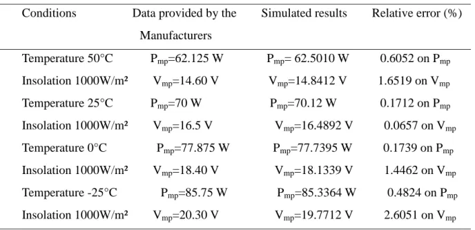
The comparison between the simulation and practical data [24] using a typical mono-crystalline solar module (Shell SP70) is illustrated in Table 2. The results show that the average relative error on peak-power voltage is 1.442225% and the average relative error on peak power is 0.358175%.
Table 1. Simulation errors on the maximum power point at different temperature (shell S75)
Conditions Data provided by the Simulated results Relative error (%) Manufacturers Temperature 50°C Pmp=66.5625 W Pmp=67.1917 W 0.9453 on Pmp Insolation 1000W/m² Vmp=15.7 V Vmp=15.5953 V 0.6669 on Vmp Temperature 25°C Pmp=75 W Pmp=74.9423 W 0.0769 on Pmp Insolation 1000W/m² Vmp=17.6 V Vmp=17.2636 V 1.9115 on Vmp Temperature 0°C Pmp=83.4375 W Pmp=82.6723 W 0.9171 on Pmp Insolation 1000W/m² Vmp=19.5 V Vmp=18.9252 V 2.9476 on Vmp Temperature -25°C Pmp=91.875 W Pmp=90.3623 W 1.6465 on Pmp Insolation 1000W/m² Vmp=21.4 V Vmp=20.5765 V 3.8479 on Vmp
Table 2.Simulation errors on the maximum power point at different temperature (shell SP70) Conditions Data provided by the Simulated results Relative error (%) Manufacturers Temperature 50°C Pmp=62.125 W Pmp= 62.5010 W 0.6052 on Pmp Insolation 1000W/m² Vmp=14.60 V Vmp=14.8412 V 1.6519 on Vmp Temperature 25°C Pmp=70 W Pmp=70.12 W 0.1712 on Pmp Insolation 1000W/m² Vmp=16.5 V Vmp=16.4892 V 0.0657 on Vmp Temperature 0°C Pmp=77.875 W Pmp=77.7395 W 0.1739 on Pmp Insolation 1000W/m² Vmp=18.40 V Vmp=18.1339 V 1.4462 on Vmp Temperature -25°C Pmp=85.75 W Pmp=85.3364 W 0.4824 on Pmp Insolation 1000W/m² Vmp=20.30 V Vmp=19.7712 V 2.6051 on Vmp 4. CONCLUSION
This study consisted in developing a new simplified model to optimize the photovoltaic solar cells. This analytical proposed model uses data provided by the constructor as a basis. Two types of solar module (Multi-crystalline silicon and mono-crystalline silicon) were modeled and evaluated. The model accuracy is also analyzed through comparison between manufacturer’s data and simulation results. The obtained results prove the efficiency of the proposed modeling approach.
5. REFERENCES
[1] M. Belhadj, T. Benouaz, A. Cheknane, S.M.A Bekkouche. Estimation de la puissance maximale produite par un générateur photovoltaïque. Revue des énergies renouvelables Vol. 13 N°2(2010) 257-264.
[2] R. Chenni, M. Makhlouf, T. Kerbache, A. Bouzid (2007). A detailed modeling method for
photovoltaic cells. Solar Energy 32: pp. 1724–1730.
[3] D.L. King, J.A. Kratochvil, W.E. Boyson, and W.I. Bower, Sandia National Laboratories. Field experience with a new performance characterization procedure for photovoltaic
arrays. Presented at the 2nd World Conference and Exhibition on Photovoltaic Solar
[4] B. S. Borowy, Z. M. Salameh, L. Pierrat and Y. J. Wang. Methodology for optimally sizing the combination of a battery bank and PV array in a wind/PV hybrid system. IEEE Transactions on Energy Conversion, vol. 11 (2), pp. 367–375, 1996.
[5] A.D. Jones and C.P. Underwood. A Modeling Method for Building-integrated Photovoltaic
Power Supply. Building Services Engineering Research and Technology, Vol. 23, N°3, pp.
167 - 177, 2002
[6] Jieming Ma, T. O. Ting, Ka Lok Man, Nan Zhang, Sheng-Uei Guan, and Prudence W. H. Wong, Parameter Estimation of Photovoltaic Models via Cuckoo Search, Hindawi Publishing Corporation Journal of Applied Mathematics Volume 2013, Article ID362619, 8 pages.
[7] M. F. AlHajri, K. M. El-Naggar, M. R. AlRashidi, and A. K. Al-Othman, “Optimal extraction of solar cell parameters using pattern search,” Renewable Energy, vol. 44, pp. 238–245, 2012.
[8] W. Huang, C. Jiang, L. Xue, and D. Song, “Extracting solar cell model parameters based on chaos particles warm algorithm,” in Proceedings of the International Conference on Electric Information and Control Engineering (ICEICE’11), pp. 398–402, April 2011. [9] A. J. Joseph, B. Hadj, and A. L. Ali, “Solar cell parameter extraction using genetic
algorithms,” Measurement Science and Technology, vol.12, no.11, pp. 1922–1925, 2001.
[10] T. F. Elshatter, M. E. Elhagree, Aboueldahab, and A. A. Elkousry, Fuzzy modeling and
simulation of photovoltaic system, in Proceedings of the 14th European Photovoltaic
Solar Energy Conference, Barcelona, Spain, 1999.
[11] A. Mellit, M. Benghanem, and SA. Kalogirou, Modeling and simulation of a stand-alone
photovoltaic system using an adaptive artificial neural network: proposition for a new sizing procedure, Renewable Energy, vol.32, no.2, pp. 285–313, 2007.
[12] A. N. Celik, “Artificial neural network modeling and experimental verification of the operating current of mono-crystalline photovoltaic modules”, Solar Energy, vol.85, no.10, pp. 2507–2517, 2011.
[13] Kon Chuen Kong, Mustafa bin Mama, Mohd. Zamri Ibrahim and Abdul Majeed
Applied Mathematical Sciences, Vol. 6, 2012, no. 8, 381 – 401.
[14] K. Tahri, B. Benyoucef. Etude de Modélisation d’un Générateur Photovoltaïque. 10ème
séminaire International sur la Physique Energétique, Journal of Scientific Research N° 0 vol. 1 (2010)
[15] Weidong Xiao, William G. Dunford, Antoine Capel. A Novel Modeling Method for
Photovoltaic Cells. 35th Annual IEEE Power Electronics Specialists Conference, 2004.
[16] D. Chan and J. Phang, “Analytical methods for the extraction of solar-cell single-and double-diode model parameters from I-V characteristics,” IEEE Transactions on Electron Devices, vol. 34, no.2, pp.286–293, 1987.
[17] D. K. Schroder, Semiconductor Material and Device Characterization, John Willey & Sons, New York, NY, USA, 1998.
[18] J. Casbestany and L. Castener, “A simple solar cell series resistance measurement method,” Revue de Physique Appliquée, vol.18, no.9, pp.565–587, 1983.
[19] Q. Jia, W. A. Anderson, E. Liu, and S. Zhang, “A novel approach for evaluating the series resistance of solar cells,” Solar Cells, vol. 25, no.3, pp.311–318, 1988.
[20] M. Bashahuand A. Habyarimana, “Review and test of methods for determination of the solar cell series resistance,” Renewable Energy, vol.6, no.2, pp.129–138, 1995.
[21] E. Saloux, A. Teyssedou, and M. Sorin, “Explicit model of Photovoltaic panels to determine voltages and currents at the maximum power point,” Solar Energy, vol.85, no.5, pp.713–722, 2011.
[22] Bryan F. Simulation of grid-tied building integrated photovoltaic systems. MS thesis, Solar Energy Laboratory, University of Wisconsin, Madison, 1999.
[23] Eckstein, J. H. Detailed modeling of photovoltaic components. MS thesis, Solar Energy Laboratory, University of Wisconsin, Madison, 1990.
[24] www.shellsolar.com
How to cite this article:
Zieba Falama R, Dadjé A, Djongyang N and Doka S.Y. A new analytical modeling method for
photovoltaic solar cells based on derivative power function. J. Fundam. Appl. Sci., 2016, 8(2),