Assessment of simplified 2D grain growth models from numerical experiments based on a level set framework

HAL Id: hal-01023803

https://hal-mines-paristech.archives-ouvertes.fr/hal-01023803

Submitted on 13 Jun 2018

HAL is a multi-disciplinary open access archive for the deposit and dissemination of sci-entific research documents, whether they are pub-lished or not. The documents may come from teaching and research institutions in France or abroad, or from public or private research centers.

L’archive ouverte pluridisciplinaire HAL, est destinée au dépôt et à la diffusion de documents scientifiques de niveau recherche, publiés ou non, émanant des établissements d’enseignement et de recherche français ou étrangers, des laboratoires publics ou privés.

Assessment of simplified 2D grain growth models from

numerical experiments based on a level set framework

Ana Laura Cruz-Fabiano, Roland E. Logé, Marc Bernacki

To cite this version:

Ana Laura Cruz-Fabiano, Roland E. Logé, Marc Bernacki. Assessment of simplified 2D grain growth models from numerical experiments based on a level set framework. Computational Materials Science, Elsevier, 2014, 92, pp.305-312. �10.1016/j.commatsci.2014.05.060�. �hal-01023803�

Assessment of simplified 2D grain growth models from numerical

experiments based on a level set framework

A.L. Cruz-Fabiano*, R. Logé and M. Bernacki

Mines ParisTech, CEMEF - Centre de Mise en Forme des Matériaux, CNRS UMR 7635, CS10207 Rue Claude Daunesse 06904 Sophia Antipolis Cedex, France

ana-laura.fabiano@mines-paristech.fr

In this paper, the results of a 2D full field grain growth model are compared with several 2D mean field grain growth models (Burke and Turbull model and Hillert/Abbruzzese model), using simplified assumptions of isotropic grain boundary energy and mobility, and under the absence of precipitates. The full field model is based on a finite element formulation combined with a level set framework, used to describe the granular structure, and model grain boundary motion through a diffusion formulation. The initial digital microstructures are created using a coupled "Voronoï-Laguerre/dense sphere packing" algorithm, which allows to obey different types of initial grain size distributions, in the considered 2D context. The results show that only the Hillert/Abbruzzese model accurately describes grain growth kinetics for all considered grain size distributions. The validity of the Burke and Turnbull model is, on the contrary, restricted to specific distributions.

Keywords: Grain growth, Full field model, Level set, Finite Element, Mean field model,

Grain size distribution

1. Introduction

Mechanical and functional properties of metals are strongly related to their microstructures, which are themselves inherited from thermal and mechanical processing. Grain growth phenomena in polycrystalline metals occur during and after full recrystallization, and have the effect of increasing the average grain size at the expense of smaller ones that will tend to disappear. Even if this phenomenon of capillarity is always present, it is generally neglected during primary recrystallization comparatively to the predominant driving force induced by the inhomogeneous spatial distribution of dislocations stored energies. Grain growth becomes however of primary importance when dealing with long annealing treatments, where capillarity effects become predominant. It then largely dictates the final grain size of the material. Over the last decades, several mesoscale numerical models have been developed to simulate the corresponding microstructure evolution [1].

Probabilistic methods associated with a voxel-based grains structure description such as of Monte Carlo (MC) [2][3] and cellular automaton (CA) [4] are widely used. Several workers have preferred to define microstructures in terms of vertices; the interface motion is then imposed by the displacement of a set of points [5]. Another approach found in the literature is the phase-field method, which offers the advantage of avoiding the difficult problem of tracking interfaces [6]. Finally, grain growth can also be modelled using a level set description of interfaces in the context of uniform grids with a finite-difference formulation [7][8] or in a finite element (FE) context [9][10], which is the method chosen in this work. First level-set simulations concerning recrystallization in polycrystalline microstructures are described in [11][12][13].

The main purpose of the paper is to test, in 2D, two mean field grain growth models existing in the literature – the one proposed by Burke and Turnbull [14], and the well-known Hillert/Abbruzzese approach [15][16][17][18] – under simplified conditions of isotropic grain

boundary energy and mobility, constant temperature, and absence of precipitates. The test is performed by comparison with the results obtained with a full field modelling method, starting from different initial grain size distributions. Grain growth models were developed based on theoretical assumptions which are not easily verified experimentally. The idea is therefore to use the full field simulations results in order to verify if and when the mean field model predictions are acceptable. If the latter are sufficiently accurate, it will also mean that full field models are not required in such simplified conditions, unless detailed topological information is needed.

In [19], R.D. Kamachali and I. Steinbach present a study with similar objectives, using a phase field framework combined with a finite-difference modelling technique. Both statistical and topological aspects of ideal grain growth, using the results of 3D simulations, are discussed. It is shown that, despite a few discrepancies with the mean field theories (Burke and Turnbull model, and Hillert model) the parabolic kinetics of grain growth remains valid during the entire process. The simulation reaches a steady state and the grain size distribution in this steady state agrees with the Hillert distribution [15]. It is also shown that the calculated volumetric growth rate compares well with the mean field assumptions. However, the paper analyzes only one initial grain size distribution, putting aside the influence of the distribution on the grain growth kinetics. In this paper, the influence of the initial grain size distribution, for equiaxed microstructures, is discussed. Thanks to a coupled “Voronoï-Laguerre/dense sphere packing” (VLDSP) algorithm [20][21], 2D imposed initial grain size distributions can be introduced accurately in the generated digital microstructures, even for a reasonable number of grains (less than 10000). Microstructures can be generated in 3D as well, leading however to unreasonable numbers of grains (in terms of computing cost) to match accurately a given grain size distribution. This remark explains why discussions addressed in the document are restricted to 2D configurations.

The paper is organized as follows. The following section explains how to generate the initial digital microstructures and immerse them in finite element meshes. It then recalls the level set framework used to describe and evolve the grain boundary network. In section 3, full field simulations are analyzed, and compared in details with the two investigated grain growth models.

2. Digital microstructures and FE immersion

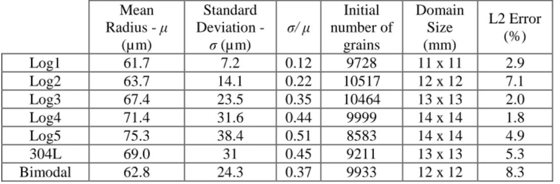
Digital microstructures are often generated using Voronoï cells [22][12]. Despite its widespread use, this classical method only allows to impose the mean grain size, and not the grain size distribution. Initial microstructures are therefore generated in this work with a VLDSP algorithm [20][21]. Seven different grain size distributions (Table 1) are studied in order to evaluate their effect on grain growth kinetics.

Mean Radius - μ (µm) Standard Deviation - σ (µm) σ/ μ Initial number of grains Domain Size (mm) L2 Error (%) Log1 61.7 7.2 0.12 9728 11 x 11 2.9 Log2 63.7 14.1 0.22 10517 12 x 12 7.1 Log3 67.4 23.5 0.35 10464 13 x 13 2.0 Log4 71.4 31.6 0.44 9999 14 x 14 1.8 Log5 75.3 38.4 0.51 8583 14 x 14 4.9 304L 69.0 31 0.45 9211 13 x 13 5.3 Bimodal 62.8 24.3 0.37 9933 12 x 12 8.3

The first five distributions are “synthetic” log normal, meaning that they are not based on real experimental data. In these cases, the mean grain size is more or less the same, and the standard deviation ranges from 7 to 40 µm. The 304L distribution was generated based on 2D experimental 304L steel data of a fully annealed sample obtained from optical microscope image analysis. It is well approximated by a log-normal law, and can therefore be compared to the first five distributions. Finally, the last distribution in Table 1 corresponds to a “synthetic” bimodal distribution. The initial number of grains is around 10000 for all distributions, which ensures a good statistics during the simulation and a reasonable numerical cost of the FE simulations (few hours in 32 CPU simulations).

Figure 1 (top) describes a comparison between the targeted microstructures and those built numerically whereas Figure 1 (bottom) illustrates the voxelized digital microstructure obtained for the bimodal case. Table 1 gives in parallel the L2 errors based on the Equation 1 below, between the theoretical and the obtained numerical distributions.

(a) (b)

Figure 1: (top) Numerical initial grain size distributions compared with the targeted ones: (a) Bimodal and 304L

distribution; (b) Log1, Log2, Log3, Log4 and Log5 distributions. In the horizontal axis the radius is normalized by the mean grain size <R>. (bottom) Voxelized digital microstructure obtained for the bimodal distribution

(1)

L2 errors increase with the complexity of the distribution and the error is more important for grains families with smaller grain size. In 2D, the Voronoï-Laguerre method consists in using a distribution of non-intersecting circular particles (generated with the dense sphere packing part of our VLDSP algorithm) that serves as a basis for constructing the grains of the polycrystal (the Voronoï-Laguerre cells). Local heterogeneities of the density of the built sphere packing, which are more likely near the smaller circles, involve local decorrelations between the imposed and the obtained cells radii. This explains the concentration of the errors in the families with smaller grain size. However the reported errors are clearly very good in comparison to the state of art [20]. It is also important to clarify that the L2 errors discussed here really correspond to a comparison between the imposed radius distribution and the equivalent radius distribution of the generated Voronoï-Laguerre cells. It is not a comparison with the generated sphere packing radius distribution, otherwise the error would always be null in the context of our LVDSP algorithm.

In order to compute the evolution of the numerical microstructures, these are discretized into a finite element mesh. Different methods can be found in the literature. The most widely used method consists in generating a surface mesh from the sides of the cell, and then generating the volume mesh starting from the surface mesh [23]. This method is relevant when modeling polycrystals deformation. However, when modeling recrystallization and grain growth, grain boundaries keep moving, grains disappear, others nucleate, etc. The complexity of the remeshing operations associated with these topological evolutions rules out the above meshing method. Ultimately, finite element methods emphasizing an explicit description of grains boundaries, such as the Vertex methods [5], always meet significant problems of mesh management, especially in 3D. Other approaches therefore favor implicit descriptions of grain boundaries, such as that introduced in the phase field [24][25] or level set methods [26][11][13][9].

In this work, a level set framework is used to implicitly describe the microstructure. A

level-set function , defined over a domain Ω, is called distance function of an interface Γ of

a sub-domain ΩS if, at any point x of Ω, it corresponds to the signed distance from Γ. In turn,

the interface Γ is given by the zero level of the function :

(2)

with the characteristic function of ΩS, equal to one in ΩS, and 0 elsewhere. According to

Equation 2, inside the domain surrounded by the interface Γ, and outside this

domain. Usually, when dealing with a polycrystalline aggregate, a distinct level set function is

used for each grain: , with NG the total number of grains in the aggregate. In

[20], the authors explain in details how the level-set function of each grain can be evaluated when the polycrystal is inserted into a finite element mesh. In this framework, the norm of the

gradient of each initial distance function is equal to one .

The use of a single level set function for each grain may lead to unreasonable computation time, when dealing with statistical numbers of grains as done here. Therefore, a graph coloration technique is used for limiting the number of level set functions needed to

 















describe the microstructure [20][27]. The objective is to use a single level set function to

describe several non-neighbouring grains, instead of just one. This brings the total number NG

of level set functions to a reduced number NC of “container” level set functions. Figure 2

illustrates a 2D 2000-grains polycrystal described using only five level set functions. In this Figure, each colour represents one container level set function.

Figure 2: A 2000-grain 2D equiaxed polycrystal described using five level set functions, as shown by the 5

different colors.

The above technique however presents the limitation that when two grains belonging to the same container level set function start touching each other, they coalesce. In [7], a method is proposed to avoid this problem: when two different grains belonging to the same container level set function get closer than a critical distance, one of the two grains is removed from the container level set function, and placed into another one. However, if the proposed methodology is applicable in the context of regular grids where the connected components (the individual grains) of each container level set function can easily be extracted, the problem becomes much more complex when dealing with non-uniform FE meshes. Therefore, in this work, it was chosen to delay the onset of grains coalescence by introducing a constraint in the

graph coloration, such that only the 4th nearest neighbour can belong to the same container

level set function. The simulation is then stopped as soon as two grains begin to coalesce. With this approach, the 10000 grains microstructure can be fully described using only around 30 container level set functions.

As stated earlier, grain boundary mobility and energy are considered isotropic and uniform throughout the domain. Grain boundaries motion can be described by Equation 3 [28][29]:

Δ , (3),

where the subcript denotes now the set of the container level-set functions, M is the grain

boundary mobility, the driving force per unit area and the outward unit normal of the

boundaries of the grains constituting the container level-set function. Considering only

grain growth, the driving force is defined by :

i f  n_i i f 

Δ , (4)

where is the grain boundary energy, and the mean curvature of the grains constituting

defined by:

. (5)

If container level set functions remain distance functions (i.e. ) near the grain

interfaces, the mean curvature can be simplified from (5) as the opposite of the Laplacian of the corresponding container level set function [9]. The grain boundary convection problem with the velocity field defined in Equation 3 is then simplified and becomes a simple diffusion problem:





The system (6) is solved for the NC container level set functions present in the domain Ω.

It describes a pure grain growth problem if and only if the metric property ( ) of each

container level set function is enforced at all time steps near the zero isovalues. This is done by using a re-initialization treatment [30] at each time step and for each container level set function.

As the diffusion of the container level set function can generate some kinematic incompatibilities at multiple junctions [26], leading to vacuum or overlapping regions, a multiple junction treatment is performed to avoid these phenomena. This multiple junction treatment is detailed in [9].

Using the numerical tools presented above, the following grain growth algorithm is proposed and is solved for each active container level set function:

GG1 – Resolution of Equation 6;

GG2 – Numerical treatment of the kinematic incompatibilities; GG3 – Re-initialization procedure;

GG4 – Deactivation if it is negative over the whole domain, i.e. when all grains of the container level-set have disappeared.

This global strategy was tested and validated for academic test cases in [9].

3. Results and discussion

For all simulations presented here and referring to the 304L steel properties, the time

step is 120 seconds, the temperature is 1050oC, with M = 1.37 10-12 m4/(J.s) [31], and γ = 0.6

J/m2. The finite element mesh is isotropic unstructured with mesh size equal to 0.01 mm over

a square domain of 13 mm x 13 mm, leading to around 8,000,000 mesh elements. Figure 3 illustrates the initial and final grain structures of 304L steel considering a 5 hours thermal treatment at 1050°C.

g

(a) (b)

(c) (d)

Figure 3: (a) Initial 304L microstructure generated with the Voronoï-Laguerre method, as shown in Figure 1b,

(b) zoom of the initial 304L microstructure, (c) simulated grain growth after 5h at 1050°C, (d) zoom of simulated grain growth.

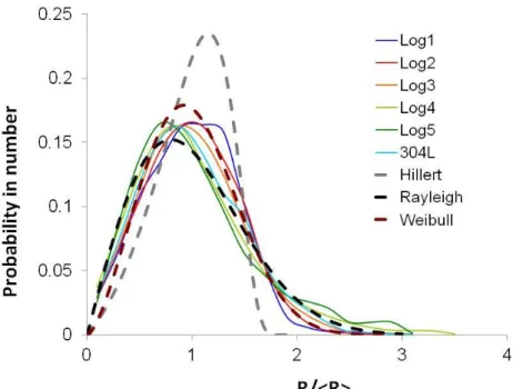
All studied distributions – except for the Bimodal (which will be discussed later) – reach at some point a quasi-steady state i.e. converge toward a quasi-constant distribution until the number of grains becomes insufficient to consider the microstructure as representative. The final grain size distributions calculated from the six initial distributions are compared with the Hillert [15], the Rayleigh and the Weibull distributions [32], [33], [34] in Figure 4. The Rayleigh distribution was originally derived in the 2D grain growth context by Louat [35] and corrected by Mullins in [36]. The Weibull distribution function has two free parameters, α and β. In [33], based on numerical simulation results, the authors found that the quasi-steady state grain size distribution is best represented using the Weibull distribution with α = 1/[Γ(1+1/β)], where Γ is the gamma function, and β = 2.5. Table 2 gives the expressions of these theoretical stationary distributions in 2D. The Hillert distribution has a

non-analytic cutoff at = 2, while the others distributions present an infinite tail.



R

Hillert distribution (7) Rayleigh distribution (8) Weibull distribution                                                   _   _RR R R R R P_w exp 1 (9)

Table 2: Hillert, Rayleigh and Weibull distribution equations.

Figure 4: Quasi-steady state and comparison with Hillert, Rayleigh and Weibull predictions.

In Figure 4, the obtained numerical quasi-steady state distributions vary between the Rayleigh and the Weibull distributions. As a conclusion, for the simulations presented in this work, the quasi-steady state grain size distribution is well represented using the Weibull distribution with a β value ranging between 2 and 2.5. On the other hand, the Hillert

distribution does not agree with the numerical results. According to Mullins [36], the reason for

the discrepancy between the Hillert theoretical distribution and the experimental and/or numerical results comes from topological reasons: in 2D, the Hillert distribution is reached only if the average number of sides relates linearly to the grain size. The relationship between the number of sides and the grain size in the results presented in Figure 4 should therefore be the subject of future work.                                     R R R R R R e R R P_H 2 4 exp 2 2 4 2 3                                   2 exp 4 2 R R R R R R P_R  

Burke and Turnbull model [10]

This model is based on three main hypotheses:

 The driving force for grain growth is proportional to the grain boundary mean

curvature approximated as , where R is the equivalent radius. So the grain

boundary migrates toward the centre of its curvature, which in turns reduces the interfacial area as well as its associated energy;

 The mobility and grain boundary energy are isotropic and uniform. As a

consequence the equilibrium angles in the triple junctions are equal to 120o;

 The heat treatment temperature is constant.

These hypotheses lead to the following grain growth kinetics equation in 2D:

, (10)

where (resp. ) corresponds to the average grain radius (resp. at t = 0s). With this

equation, neither the topological nor the neighbouring effects are taken into account; the grain growth kinetics is characterized only by the average grain size.

To check the consistency between the full field simulation results and this model, the curves log









(11).

From Equation 11, the validity of the Burke and Turnbull model can be verified if the slope n

of log









2

t f R

R   , is equal to 1, and if the fitted curve leads to an α value around 0.5.

Computed curves and their linear fits are given in Figure 5 and lead to the α and n parameters summarized in Table 3.

Distribution Slope (n) α Number of grains in the end Log1 2.48 1.21 10-7 4078 Log2 1.59 1.08 10-3 3747 Log3 1.19 0.08 2889 Log4 1.02 0.38 2782 Log5 0.89 2.3 2743 304L 1.04 0.42 3271

Table 3: Burke and Turnbull model analysis by comparison with full field simulations results, considering six

different initial grain size distributions (described in Table 1).

      R 1 t M R R  2 1 ² 02  R R0 n t M R R² 02 





Figure 5: Computed evolutions of grain structures starting with different initial grain size distributions, using

the full field model. Linear approximations are added for comparison with the Burke and Turnbull model.

As illustrated in Table 3 and Figure 5, n and α are highly dependent on the initial grain size distribution. Only the Log4 and 304L distributions lead to the values of n and α expected by the Burke and Turnbull model. Both distributions are log-normal with a value of

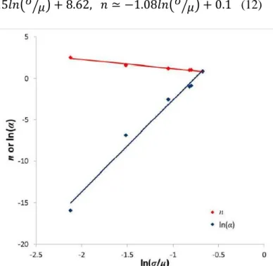
(see Table 1). For the other distributions, it can be noticed in Figure 6 that n

values decrease with the increase of , while α values increase with . These

evolutions can be approximated by the following simple relationships:

(12)

Figure 6: Relationship between α and n fitted parameters and σ/μ of the initial grain size distributions (given in

Table 1) 45 . 0       

Thus for a log-normal distribution, presents a power law dependence on and n a logarithmic dependence. Equations 12 confirm that grain growth kinetics significantly depends on grain structure and neighbourhood effects. Using the numerical grain growth results we propose a correction of the Burke and Turnbull model. Once Equations 11 are experimentally verified, this corrected Burke and Turnbull model can be directly used when modelling grain growth phenomena.

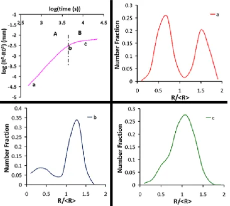
Figure 7 shows that the Bimodal kinetics can be divided into 2 linear parts – ‘A’ and ‘B’. Evolution of the grain size distributions is also given at different times ‘a’ (t = 0s), ‘b’ (t = 4400s) and ‘c’ (t = 18000s). The slope change in the kinetics is seen to coincide with the quasi disappearance of the smallest grains population, i.e. with the switching from a bimodal distribution to a single peak distribution.

Figure 7: (Top to botton and left to right) Burke and Turnbull model study for Bimodal distribution; grain size

distribution at point a (t = 0 s), at point b (t = 4400 s), and at point c (t = 18000 s).

It is therefore concluded that the Burke and Turnbull model is not valid for most of the investigated grain size distributions. The model only behaves well for lognormal grain size

distributions, with a value close to 0.45.

Hillert/Abbruzzese model

Hillert [15] and Abbruzzese [16][17][18] mean field models are derived from the von Neumann-Mullins theory [37][38]. Even though the proposed developments differ, both Hillert and Abbruzzese models finally propose the same grain growth Equation 13. Therefore, no distinction is done here between these two approaches. The central equation is:

        i i R R M R   1 1 , (13)



where the grain structure is assumed to be described by a discrete set of grain families (each

family being labeled with a subscript i), corresponds to the average grain boundary

velocity of the grain family i, corresponds to the average grain size and is a constant

generally assumed to be 0.5 in 2D, and 1 in 3D, even though other values can be found in the literature. For example, in [19], Kamachali found a value of 1.25 in 3D, using a phase field framework combined with a finite-difference modelling technique. In [39], Rios and Glicksman calculated a 3D value of 0.81, using the average N-hedra method (ANH) [40].

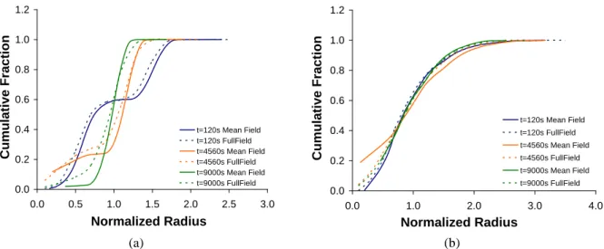
To check the consistency between the full field simulations and the Hillert/Abbruzzese model, calculated grain size distributions are compared. The mean field computations are based on Equation 12, implemented within a more general model described in [41] where . Three different times (t = 2 min, t = 76 min and t = 150 min) were analysed, for all initial grain size distributions considered in Table 1. The corresponding L2 errors (see Equation 1) are given in Table 4. They are based on cumulative distribution functions, as illustrated in Figure 8 for the Bimodal and the 304L cases.

Error L2 (%)

t = 2 min t = 76 min t = 150 min Log1 10.7 4.6 3.9 Log2 4.5 4.6 6.3 Log3 1.9 4.0 6.0 Log4 1.6 4.5 7.6 Log5 1.9 2.4 3.4 304L 1.9 5.5 5.5 Bimodal 4.9 6.8 10.3

Table 4: L2 Errors between grain size distributions obtained with the full field model, and with the

Hillert/Abbruzzese mean field model. Errors are computed based on the cumulative distribution functions (see Figure 8).

(a) (b)

Figure 8: Comparison between full field results and Hillert/Abbruzzese mean field results for (a) Bimodal, and

(b) 304L distributions. Results are displayed using cumulative distribution functions.

From Table 4, it can be concluded that the Hillert/Abbruzzese mean field model is overall in good agreement with the full field computations. L2 errors remain below 11% for all considered distributions, including the Bimodal one. A closer look at the distributions, e.g. those illustrated in Figure 8, shows that errors increase in the lowest grain sizes range. An hypothesis which explains this error is related to volume conservation issues discussed in [41]: volume changes of the shrinking grains are computed by redistributing the total volume changes of growing grains. Consequently, the rates of volume change for small grain sizes are

i R R 0.0 0.2 0.4 0.6 0.8 1.0 1.2 0.0 0.5 1.0 1.5 2.0 2.5 3.0 Normalized Radius Cumulative Frac tion t=120s Mean Field t=120s FullField t=4560s Mean Field t=4560s FullField t=9000s Mean Field t=9000s FullField 0.0 0.2 0.4 0.6 0.8 1.0 1.2 0.0 1.0 2.0 3.0 4.0 Normalized Radius Cumulative Frac tion t=120s Mean Field t=120s FullField t=4560s Mean Field t=4560s FullField t=9000s Mean Field t=9000s FullField

slightly modified from the values strictly deriving from Equation 12. Comparing the results obtained using the mean field model discussed in [41] and the direct use of Equation 12, it is observed that the effect of the volume conservation treatment is more important for a small number of representative grain families (around 50). In fact, when using 40 representative grain families (as the case in the comparisons presented in Figure 8), the direct use of Equation 12 gives better results than the model presented in [41]. However, for a statistical number of representative grains around 200, both methods lead to the same results, and the volume conservation treatment does not affect the results. A more complete study of the volume conservation issue will be the subject of future work.

Full field computations give a β value (Equation 12) around 0.5 which is exactly the expected value.

It is therefore concluded that, in the absence of second phase particles and under simplifying conditions of uniform and isotropic grain boundary energy and mobility, the Hillert/Abbruzzese mean field model describes grain growth with good accuracy, for a wide range of initial grain structures.

4. Conclusions

The validity of two grain growth models has been discussed based on full field model computations. The full field model is based on a finite element formulation combined with a level set framework. Seven initial grain size distributions have been considered in order to test the investigated grain growth models. Computed quasi-steady state distributions compare well with the Weibull distribution with a β value ranging between 2 and 2.5, and significantly differ from the Hillert distribution.

The simplified Burke and Turnbull model is shown to be valid only for two grain size distributions. Both of them are lognormal and present a standard deviation value equal to 0.45 times the average grain size. It can be noticed that this kind of distribution is classically observed in polycrystalline metals. On the other hand, the Hillert/Abbruzzes model is shown to be accurate for all tested distributions, even the Bimodal one. Consequently, if the development of full field models is justified for the description of grain growth in complex conditions, or for complex microstructures, their use appears disproportionate in the simple configurations investigated here, where the Hillert/Abbruzzese model behaves very well.

It is important to highlight that all conclusions presented in this work are valid under simplified conditions: 2D grain growth, isotropic grain boundary mobility and energy and no dragging forces. In order to verify if these conclusions are still valid under more complex and realistic conditions (3D grain growth, anisotropic grain boundary mobility and energy, etc.), complementary numerical simulations and/or experimental tests must be performed.

Future work will be dedicated to (i) investigating volume conservation issues in grain growth regime, (ii) analyzing the number of sides relationship with the grain size, particularly in the quasi-steady regime, (iii) extending the present study from 2D to 3D, (iv) considering anisotropic grain boundary mobility and energy, and (v) following the same strategy to compare static and dynamic recrystallization predictions of the mean field model presented in [41] with those obtained with the full field approach [12][13].

References

[1] M.A. Miodownik, J. Light Metals 2 (2002) 125.

[2] A.D. Rollet, D. Raabe, Comput. Mater. Sci. 21 (2001) 69.

[4] D. Raabe, Phil. Mag A. 79 (1999) 2339.

[5] L.A. Barrales, G. Gottstein, L.S. Shvindlerman, Acta Mater. 56 (2008) 5915. [6] L.Q. Chen, Ann. Rev. Mater. Res. 32 (2002) 113.

[7] M. Elsey, S. Esedoglu, P. Smereka, J. Comput. Phys. 228 (2009) 8015. [8] M. Elsey, S. Esedoglu, P. Smereka, Acta Mater. 61 (2013) 2033. [9] M. Bernacki, R. Loge, T. Coupez, Scripta Mat. 64, (2011) 525.

[10] A. Agnoli, M. Bernacki, R. Logé, J.-M. Franchet, J. Laigo, N. Bozzolo, Understanding and modeling of grain boundary pinning in Inconel 718, Proceedings

of the 12th International Symposium on Superalloys.

[11] M. Bernacki, Y. Chastel, T. Coupez, R.E. Logé, Scripta Mat. 58 (2008) 1129.

[12] R.E. Logé, M. Bernacki, H. Resk, L. Delannay, H. Digonnet, Y. Chastel, T. Coupez, Philos. Mag. 88 (2008) 3691.

[13] M. Bernacki, H. Resk, T. Coupez, R.E. Logé, Model. Simul. Mater. Sci. Eng. 17 (2009) 064006.

[14] J.E. Burke, D. Turnbull. Progress in Metal Physics. 3 (1952) 220. [15] M. Hillert. Acta Metall. Mat.13 (1965) 227.

[16] K. Lücke, R. Brandt, G. Abbruzzese. Interface Science. 6 (1998) 67.

[17] G. Abbruzzese, I. Heckelmann, K. Lücke. Acta Metallurgica et Materialia. 40 (1992) 519.

[18] K. Lücke, I. Heckelmann, G. Abbruzzese. Acta Metallurgica et Materialia, 40, (1992) 533.

[19] R.D. Kamachali, I. Steinbach, Acta Mat. 60 (2012) 2719.

[20] K. Hitti, P. Laure, T. Coupez, L. Silva, M. Bernacki, Comp. Mater. Sci. 61 (2012) 224.

[21] K. Hitti, M. Bernacki, App. Math. Model. 37 (2013) 5715.

[22] P.R. Dawson, M.P. Miller, T.S. Han, J. Bernier, Metall. Mater. Trans. A 36 (2005) 1627

[23] A.D. Rollett. Proc. Conf. Numiform, Columbus. (2004) 71. [24] Y. Suwa, Y. Saito, H. Comput. Mater. Sci. 44 (2008) 286.

[25] T.Takaki, Y.Tomita. International Journal of Mechanical Sciences, vol. 52, pp. 320– 328, 2010.

[26] B. Merriman, J. Bence, S. Osher, J. Comput. Phys. 112 (1994) 334.

[27] M. Kubale, American Mathematical Society, Providence, Rhode Island, 2004. [28] G. Kugler, R. Turk, Acta Mater. 52 (2004) 4659.

[29] G. Kugler, R. Turk, Comput. Mater. Sci. 37 (2006) 284. [30] J.A. Sethian, Cambridge University Press. (1996).

[31] M. El Wahabi, J.M. Cabrera, J.M. Prado. Mater. Sci. and Engng. A. 343 (2003) 116. [32] P.R. Rios, Scripta Mater. 40 (1999) 665.

[33] W. Fayad, C.V. Thompson, H.J. Frost, Scripta Mater. 40 (1999) 1199. [34] P.R. Rios, Scripta mater. 42 (2000) 349.

[35] N.P. Louat, Acta metall. 22 (1974) 721. [36] W. W. Mullins, Acta. Mater. 46 (1998) 6219. [37] W. W. Mullins, J. Appl. Phys. 27 (1956) 900.

[38] J. von Neumann, in Metals Interfaces, ASM, Cleveland, Ohio. (1952) 108. [39] P.R. Rios, M.E. Glicksman. Acta Materialia (2008).

[40] M.E. Glicksman. Philos Mag. (2005).