Funchal, Madeira, September 1-3, 2011
SUBPROBLEM FINITE ELEMENT METHOD FOR
MAGNETIC MODEL REFINEMENTS
Patrick Dular1,2, Mauricio V. Ferreira da Luz3, Patrick Kuo-Peng3, Ruth V. Sabariego1,
Laurent Krähenbühl4 and Christophe Geuzaine1
1University of Liège, Dept. of Electrical Engineering and Computer Science, ACE, B-4000 Liège, Belgium 2F.R.S.-FNRS, Fonds de la Recherche Scientifique, Belgium
3GRUCAD/EEL/UFSC, Po. Box 476, 88040-970 Florianópolis, Santa Catarina, Brazil
4 Université de Lyon, Ampère (CNRS UMR5005), École Centrale de Lyon, F-69134 Écully Cedex, France
Abstract⎯ Model refinements of magnetic circuits are performed via a subproblem finite element method.
A complete problem is split into subproblems with overlapping meshes, to allow a progression from source to reaction fields, ideal to real flux tubes, 1-D to 2-D to 3-D models, perfect to real materials, with any coupling of these changes. Its solution is the sum of the subproblem solutions. The procedure simplifies both meshing and solving processes, and quantifies the gain given by each refinement on both local fields and global quantities.
Introduction
The finite element (FE) subproblem method (SPM) provides advantages in repetitive analyses and helps improving the solution accuracy [1-6]. It allows to benefit from previous computations in-stead of starting a new complete FE solution for any geometrical, physical or model variation. It al-so allows different problem-adapted meshes and computational efficiency due to the reduced size of each SP. A general framework allowing a wide variety of refinements is herein presented. It is a FE SPM based on canonical magnetostatic and magnetodynamic problems solved in a sequence, with at each step volume sources (VSs) and surface sources (SSs) originated from previous solu-tions. VSs express changes of material properties. SSs express changes of boundary conditions (BCs) or interface conditions (ICs). Common and useful changes from source to reaction fields, ideal to real flux tubes (with leakage flux), 1-D to 2-D to 3-D models, perfect to real materials, and statics to dynamics, can all be defined via combinations of VSs and SSs. The developments are per-formed for the magnetic vector potential FE formulation, paying special attention to the proper dis-cretization of the constraints involved in each SP. The method is illustrated and validated on vari-ous problems.
Sequence of Coupled Subproblems
Canonical Magnetodynamic/static Problem
A complete problem is split into a series of SPs that define a sequence of changes, with the com-plete solution being replaced by the sum of the SP solutions. Each SP is defined in its particular domain, generally distinct from the complete one and usually overlapping those of the other SPs. At the discrete level, this aims to decrease the problem complexity and to allow distinct meshes with suitable refinements. No remeshing is necessary when adding some regions.
A canonical magnetodynamic/static problem p, to be solved at step p of the SPM, is defined in a domain Ωp, with boundary ∂Ωp=Γp=Γh,p∪Γb,p. The eddy current conducting part of Ωp is
denot-ed Ωc,p and the non-conducting one Ωc,pC, with Ωp=Ωc,p∪Ωc,pC. Massive inductors belong to
Ωc,p, whereas stranded inductors belong to Ωc,pC. The equations, material relations and boundary
conditions (BCs) of problem p are
curlhp=jp , divbp=0 , curlep=–∂tbp , (1a-b-c)
hp=µp–1bp+hs,p , jp=σpep+js,p , (2a-b)
n×hp|Γh,p=jf,p, n⋅bp|Γb,p=ff,p, n×ep|Γe,p⊂Γb,p=kf,p, (3a-b-c)
where hp is the magnetic field, bp is the magnetic flux density, ep is the electric field, jp is the elec-tric current density, µp is the magnetic permeability, σp is the electric conductivity and n is the unit
normal exterior to Ωp. Note that (1c) is only defined in Ωc,p (as well as ep), whereas it is reduced to
the form (1b) in Ωc,pC. It is thus absent from the magnetostatic version of problem p. Further (3c)
is more restrictive than (3b) in their homogeneous forms. Equations (1b-c) are fulfilled via the def-inition of a magnetic vector potential ap and an electric scalar potential vp, leading to the ap
-formulation, with
curlap=bp , ep=–∂tap–gradvp , n×ap|Γb,p=af,p . (4a-b-c)
For various purposes, some paired portions of Γp can define double layers, with the thin region in
between exterior to Ωp [2-5]. They are denoted γp+ and γp– and are geometrically defined as a
sin-gle surface γp with ICs, fixing the discontinuities ([⋅]γp=⋅|γp+ –⋅|γp–)
[n×hp]γp=[jf,p] , [n⋅bp]γp=[ff,p] , [n×ep]γp=[kf,p] and [n×ap]γp=[af,p] . (5a-b-c-d)
With the definitions (nγp≡n|γp)=–(n
+≡n|
γp+)=(n
–≡n|
γp–) for the normal n in different contexts, one
has, e.g. for (5a),
[n×hp]γp=nγp×hp|γp+ –nγp×hp|γp– =–(n+×hp|γp+ –n–×hp|γp–). (6)
The fields hs,p and js,p in (2a-b) are volume sources (VSs). The source hs,p is usually used for fix-ing a remnant field in magnetic materials. The source js,p fixes the current density in inductors.
With the SPM, hs,p is also used for expressing changes of permeability and js,p for changes of
con-ductivity, or for adding portions of inductors [2-6]. For changes in a region, from µq and σq for
problem q to µp and σp for problem p, the associated VSs hs,p and js,p, limited to the modified
re-gions, are
hs,p=(µp–1–µq–1)bq , js,p=(σp–σq)eq , (7a-b)
for the total fields to be related by the updated relations hq+hp=µp–1(bq+bp) and
jq+jp=σp(eq+ep).
The surface fields jf,p, ff,p and kf,p in (3a-c), and af,p in (4c), are generally zero for classical
homo-geneous BCs. The discontinuities (5a-d) are also generally zero for common continuous field trac-es. If nonzero, they define possible surface sources (SSs) that account for particular phenomena oc-curring in the thin region between γp+ and γp– [2-5]. This is the case when some field traces in a
problem q are forced to be discontinuous. The continuity has to be recovered after a correction via a problem p. The SSs in problem p are thus to be fixed as the opposite of the trace solution of prob-lem q.
Each problem p is to be constrained via the so defined VSs and SSs from parts of solutions of other problems. This is a key element of the SPM, offering a wide variety of possible corrections, as shown hereafter.
The complete solution is
u = up
p!P
"
, with u # h, b, j, e, ... (8)with P an ordered set of SPs. A correction can become a significant source for any of its source problems, which is inherent to large perturbation problems. In this case, an iterative process be-tween the related SPs has to be done till convergence up to a desired accuracy [4]. In addition to the iterations between SPs, classical inter-problem iterations are needed in nonlinear analyses. Each so-lution up can then be calculated as a series of corrections up,i (with i the sub-SP (SSP) index), i.e.
up= up,i
i
Finite Element Weak Formulations
The weak ap-formulation of the canonical problem p is obtained from the weak form of the Am-père equation (1a), i.e. [2-5],
(µ!1p curl ap, curl a')"p+ (hs, p, curl a')"p!( js, p, a')"p +(!p!tap, a')"c, p
+< n ! hs, p, a' >"h, p+< n ! hp, a' >"b, p +< ![n " hp]!p, a' >!p= 0 , ! a' " Fp
1
(#p), (10) where Fp1(Ωp) is a curl-conform function space defined on Ωp, gauged in Ωc,pC, and containing the
basis functions for a as well as for the test function a' (at the discrete level, this space is defined by edge FEs; the gauge is based on the tree-co-tree technique); (·,·)Ω and <·,·>Γ respectively de-note a volume integral in Ω and a surface integral on Γ of the product of their vector field argu-ments. The surface integral term on Γh,p accounts for natural BCs of type (3a), usually zero.
The term on the surface Γb,p with essential BCs on n⋅bp is usually omitted because it does not
lo-cally contribute to (10). It can be used for post-processing a solution, a part of which n×hp|Γb,p
hav-ing to act further as a SS [2-5].
Some parts of a previous solution aq serve as VSs and SSs in a subdomain Ωs,p⊂Ωp of the current
problem p. At the discrete level, this means that this source quantity aq has to be expressed in the mesh of problem p, while initially given in the mesh of problem q. This is done via an L2 -projection [8] of its curl limited to Ωs,p, i.e.
(curlaq-p,curla')!
s, p=(curlaq,curla')!s, p, "a' # Fp
1(!
s, p) , (11)
where Fp1(Ωs,p) is a gauged curl-conform function space for the p-projected source aq-p (the
pro-jection of aq on mesh p) and the test function a'.
VSs for changes of material properties and inductors – A change of material properties from SP q to SP p is taken into account in (10) via the source integrals (hs, p, curl a')!
p and ( js, p, a')!p. The
VSs hs,p and js,p are respectively given by (7a) and (7b), i.e. hs,p=(µp–1–µq–1)bq and js,p=(σp–
σq)eq with (4a-b), bq=curlaq and ep=–∂tap (vp can be generally omitted). A change of current
density directly defines the related VS js,p. At the discrete level, the source primal quantity aq, ini-tially given in mesh q, is projected in the mesh p via (11), with Ωs,p limited to the modified regions.
SSs for changes of BCs or ICs –
Both essential and natural BCs or ICs are to be considered, respectively (4c) or (5d), and (3a) or (5a). Essential conditions can be directly applied, whereas natural conditions gain at being applied in an indirect way, avoiding to locally evaluate the weak trace of hp on the related surfaces. Usually, the trace discontinuity of hp is defined as the opposite of the trace discontinuity of a previous solution hq (or a sum of previous solutions), i.e.[n×hp]γp=–[n×hq]γq≡γp , or [n×hp]γp=–n×hq|γq+≡γp+ , (12a-b)
or respectively, in the related integral term in (10), < ![n " hp]!
p, a' >!p=< [n " hq]!q, a' >!q#!q, or < ![n " hp]!p, a' >!p=< n " hq, a' >!q+#!q+. (13a-b)
The RHS term of (13a-b), on this weak form, is just a term that occurs in the weak formulation of SP q, of form (10) written for SP p≡q. It can thus be naturally expressed via the volume integrals of this formulation, i.e. usually, with Γb,q=γp, e.g.
< n ! hq, a' >!q= "(µq
"1curl a
q, curl a')#p$#q"(!q%taq, a')#c, p$#c,q. (14)
The weak nature of the natural BC or IC is thus conserved. At the discrete level, the volume inte-grals in (14) are limited to one single layer of FEs touching γq for (13a) or γq+ for (13b) (thus
re-spectively on both sides or on one side of γq), because they involve only the associated traces
n×a'|γq or n×a'|γq+. The source aq, initially in mesh q, has to be projected in mesh p via (11), with
Ωs,p limited to the FE layer, which thus decreases the computational effort of the projection
Various Correction Schemes
Various correction schemes, appropriate to practical magnetic system analyses, can benefit from the developed SPM.
Change of material properties
A typical problem is that of a region put in an initially calculated source field b1 (SP 1, Fig. 1). The associated SP 2 is solved in its proper mesh, with the added core and its surrounding region, and VSs (2a) and/or (2b) limited to this core, where µ and/or σ are modified, from µ1 to µ2 and/or σ1 to σ2. Such changes can occur when adding or suppressing materials or portions of those, in, e.g., shape optimization, non-destructive testing, moving systems [6].
A change from a linear to a nonlinear magnetic material is a particular case of a change or permea-bility (Fig. 2), requiring classical nonlinear iterations for the related nonlinear SP.
From the so calculated field corrections, the associate corrections of global quantities inherent to magnetic models, i.e. fluxes, magnetomotive forces (MMFs), currents and voltages, can be evaluat-ed.
Fig. 1. Field lines for an inductor alone (b1, left) and for an added core (b2, µr,core = 100) (right); distinct
meshes are used for SPs 1 and 2.
Fig. 2. Field lines and magnetic flux density for a linear model (b1, µr,1=1000, top left) and its non-linear
cor-rection (b2, top right); another non-linear correction (b2, from µr,1=780, bottom right); final relative
Change from ideal to real flux tubes
A SP q can first consider ideal tubes [7], i.e. surrounded by perfect flux walls through which
n⋅bq|γq is zero and bq and hq outside are zero [3-4]. The complementary trace n×hq|γq is unknown
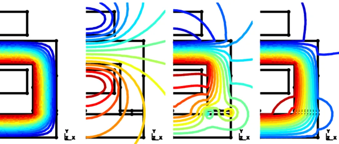
and non-zero. Consequently, a change to a permeable flux wall defines a SP p with SSs opposed to this non-zero trace. This change can be done simultaneously with a material change (Fig. 3): a leakage flux solution b3 can complete an ideal distribution b1 while knowing the source b2 proper to the inductor; this allows independent overlapping meshes for both source and reaction fields.
Fig. 3. An electromagnet: field lines in an ideal flux tube (b1, µr,core = 100), for the inductor alone (b2), for the
leakage flux (b3) and for the total field (b=b1+b2+b3) (left to right).
Change from 1-D to 3-D
The SPM can be applied for coupling solutions of various dimensions, starting from simplified models, based on ideal flux tubes defining 1-D models, that evolve towards 2-D and 3-D accurate models [5].
Series connections of models of lower dimensions are direct applications requiring such changes. A violation of ICs when connecting two models can be corrected via SSs in opposition to the unwant-ed discontinuities. An accurate series connection of two 1-D flux tubes neunwant-eds a changes from 1-D to 2-D (Fig. 4). Also, the connection of 2-D models needs a 3-D correction model for an accurate consideration of 3-D effects (Fig. 5).
Change from ideal to real flux tubes can be extended to allow a dimension change, e.g. from 2-D to 3-D (Fig. 6): a 2-D solution is first considered as limited to a certain thickness in the third dimen-sion, with a zero field outside; on the other side, another independent SP is solved. Changes of ICs on each side of this portion, via SSs, then allow the calculation of 3-D end effects. The successive corrections of the flux linkage, from 1-D to 3-D, are shown in Fig. 7.
Fig. 4. Series connection of two flux tubes: field lines in 1-D ideal flux tubes (b1, left), 2-D local correction at
Fig. 5. Field lines (left) generated by a stranded inductor (half geometry): solution of a 2-D plane model in the XY plane (z = 0) (b1, portion on the left) and of a 2-D axisymmetrical model in the YZ plane (x = 0) (b2,
portion on the right); the interface between the two portions is shown. Magnetic flux density (right) along the coil axis in the 3-D system: b1 for the 2-D plane model (implicitly extended as a constant up to z= 100mm),
b2 for the 2-D axisymmetrical model, b3 for the 3-D correction and b for the complete 3-D model. The
solu-tion b1+b2+b3 is generally obtained with a higher accuracy than b for a lower computational cost thanks to the
coupling of meshes, some of lower dimensions.
Y X Z Y Z X
Fig. 6. 3-D model of an electromagnet (left), 2-D cross section and solution (magnetic flux density and field lines) (middle), 3-D correction of the magnetic flux density (right).
0 0.1 0.2 0.3 0.4 0.5 0.6 0.7 0.8 1 10 100 1000 Magnetic flux \ (mWb)
Relative magnetic permeability µr,core
gap 3mm 3-D 1-D 2-D, ideal tube 2-D, leakage in 2-D, leakage in+out 0.1 1 10 100 1000 1 10 100 1000 Relative correction 2-D/1-D (%)
Relative magnetic permeability µr,core
gap 3mm gap 1mm gap 0mm 0.1 1 10 100 1 10 100 1000 Relative correction 3-D/2-D (%)
Relative magnetic permeability µr,core
gap 3mm
gap 1mm gap 0mm
Fig. 7. Inductor flux linkage versus the core magnetic permeability (air gap thickness of 3 mm) updated after each model refinement (left); flux linkage relative correction from 1-D to 2-D models (middle) and from 2-D to 3-D models (right) versus the core magnetic permeability for different air gap thicknesses.
Change from perfect to real materials
A SP q can first consider perfect conducting (resp. magnetic) materials [2], with σq→∞ (resp.
µq→∞), in which case the trace n⋅bq|γq (resp. n×hq|γq) on its boundary is zero and bq (resp. hq)
in-side is zero. The complementary trace n×hq|γq (resp. n⋅bq|γq) is unknown and non-zero.
Conse-quently, a change to a finite σp (resp. µp) defines a SP p with SSs opposed to this non-zero trace.
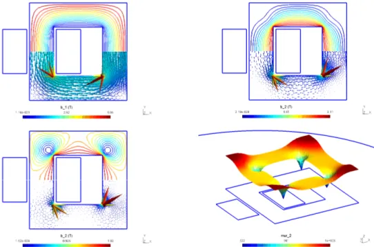
As an illustration, an induction heating core-inductor system is initially modeled with a perfectly conducting core, then corrected for a finite conductivity (Fig. 8). After correction, a very good ac-curacy, in particular in the vicinity of the conductor corners, is obtained (Fig. 9), also in compari-son with the impedance BC (IBC) technique. Initially perfectly conducting inductors can be also considered, followed by the correction of their eddy current density for an accurate calculation of impedance and Joule losses (Fig. 10).
Y X az (0) 1.83e-006 3.54e-006Z -2.7e-017 Y X az (0) 2.28e-007 1.32e-006Z -9.33e-007 Y X az (0) 1.7e-006 4.17e-006Z -9.33e-007
Fig. 8. Core-inductor system: magnetic flux lines for the perfectly conducting core (non-magnetic) (b1; left),
the finite conductivity correction (aluminium core) (b2; middle) and the complete solution (b=b1+b2; right).
Fig. 9. Eddy current density along the (conductive non-magnetic) core surface for the conventional FE solu-tion, the SPM and the IBC technique (top); relative difference between solutions of the last two techniques (bottom).
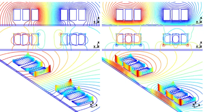
Fig. 10. Transverse flux system (3-turn inductor above a half plate, with perpendicular flux horizontal sym-metry axis below); a low (left) and a high (right) electric conductivity are considered for the plate; from top to bottom: magnetic flux lines (phase 0) for the reference solution b1 with a perfectly conductive inductor, the
perturbation solution b2 and the perturbed solutions b; bottom: current density distribution (modulus).
Conclusions
The developed SP FE method splits magnetic problems into SPs of lower complexity with regard to meshing operations and computational aspects. This allows a natural progression from simple to more elaborate models, while quantifying the gain given by each model refinement and justifying its utility.
Approximate problems with ideal flux tubes are accurately corrected when accounting for leakage fluxes and material changes. Also, reference solutions related to limit behaviors of conductors (per-fectly conductive or magnetic nature) can be used in several subproblems for accurate calculation of the field distribution in real materials and the ensuing losses. This allows efficient parameterized analyses on the electric and magnetic characteristics of the conductors in a wide range, i.e. on the parameters affecting the skin depth. Nonlinear analyses, e.g. with temperature dependent conduc-tivities, could then benefit from this. The method is naturally adapted to parameterized analyses on geometrical and material data.
All the constraints involved in the subproblems have been carefully defined in the associated FE formulations, respecting their inherent strong and weak nature. As a result, local fields and global quantities, i.e. flux, MMF, reluctance, voltage, current, resistance, are efficiently and accurately calculated.
References
[1] Z. Badics, Y. Matsumoto, K. Aoki, F. Nakayasu, M. Uesaka, and K. Miya, An effective 3-D finite element scheme for computing electromagnetic field distorsions due to defects in eddy-current nondestructive evaluation, IEEE Trans. Magn., Vol. 33, No. 2, pp. 1012-1020, 1997.
[2] P. Dular, R. V. Sabariego, J. Gyselinck, and L. Krähenbühl, Sub-domain finite element method for efficiently considering strong skin and proximity effects, COMPEL, Vol. 26, No. 4, pp. 974-985, 2007. [3] P. Dular, R. V. Sabariego, M. V. Ferreira da Luz, P. Kuo-Peng, and L. Krähenbühl, Perturbation Finite
Element Method for Magnetic Model Refinement of Air Gaps and Leakage Fluxes, IEEE Trans. Magn., Vol. 45, No. 3, pp. 1400-1403, 2009.
[4] P. Dular, R.V. Sabariego, M.V. Ferreira da Luz, P. Kuo-Peng, and L. Krähenbühl, Perturbation finite-element method for magnetic circuits. IET Science, Measurement & Technology, Vol. 2, No. 6, pp. 440-446, 2008.
[5] P. Dular, R.V. Sabariego, and L. Krähenbühl, Magnetic model refinement via a perturbation finite element method – from 1-D to 3-D, COMPEL, Vol. 28, No. 4, pp. 974-988, 2009.
[6] P. Dular and R. V. Sabariego, A perturbation method for computing field distortions due to conductive regions with h-conform magnetodynamic finite element formulations, IEEE Trans. Magn., Vol. 43, No. 4, pp. 1293-1296, 2007.
[7] C. Chillet and J.Y. Voyant, Design-oriented analytical study of a linear electromagnetic actuator by means of a reluctance network, IEEE Trans. Magn., Vol. 37, No. 4, pp. 3004-3011, 2001.
[8] C. Geuzaine, B. Meys, F. Henrotte, P. Dular and W. Legros, A Galerkin projection method for mixed finite elements, IEEE Trans. Magn., Vol. 35, No. 3, pp. 1438-1441, 1999.