arXiv:1712.02968v1 [astro-ph.SR] 8 Dec 2017
Astronomy & Astrophysicsmanuscript no. paper ESO 2017c
December 11, 2017
B stars seen at high resolution by
XMM
-
Newton
⋆
Constantin Cazorla and Yaël Nazé
⋆⋆Groupe d’Astrophysique des Hautes Energies, STAR, Université de Liège, Quartier Agora (B5c, Institut d’Astrophysique et de Géo-physique), Allée du 6 Août 19c, B-4000 Sart Tilman, Liège, Belgium
e-mail: [email protected] December 11, 2017
ABSTRACT
We report on the properties of 11 early B stars observed with gratings on board XMM-Newton and Chandra, thereby doubling the number of B stars analysed at high resolution. The spectra typically appear soft, with temperatures of 0.2–0.6 keV, and moderately bright (log[LX/LBOL] ∼ −7) with lower values for later type stars. In line with previous studies, we also find an absence of circumstellar absorption, negligible line broadening, no line shift, and formation radii in the range 2 – 7 R⋆. From the X-ray brightnesses, we derived the hot mass-loss rate for each of our targets and compared these values to predictions or values derived in the optical domain: in some cases, the hot fraction of the wind can be non-negligible. The derived X-ray abundances were compared to values obtained from the optical data, with a fair agreement found between them. Finally, half of the sample presents temporal variations, either in the long-term, short-term, or both. In particular, HD 44743 is found to be the second example of an X-ray pulsator, and we detect a flare-like activity in the binary HD 79351, which also displays a high-energy tail and one of the brightest X-ray emissions in the sample.
Key words. stars: early-type – X-rays: stars
1. Introduction
The advent of the first high-resolution X-ray spectrographs on board XMM-Newton and Chandra profoundly modified our un-derstanding of high-energy phenomena. Indeed, high-resolution spectra provide a wealth of detailed information. For massive stars, the X-ray emission comes from optically thin, hot plasma; hence lines dominate the X-ray spectra. Their relative strengths closely constrain the plasma temperature and composition. The ratios between forbidden and intercombination lines of He-like ions further pinpoint where X-rays arise (Porquet et al. 2001). Finally, their line profiles provide unique information on the stellar wind, its opacity, and its velocity field (Macfarlane et al. 1991; Owocki & Cohen 2001).
Analyses of the high-resolution spectra of O stars have revealed winds to be less opaque than initially thought and have helped constraining the properties of high-energy interac-tions (e.g. colliding winds in binaries and magnetically confined winds in strongly magnetic objects). However, many fewer B stars were observed at high resolution. To further advance the un-derstanding of X-rays associated with early B stars, we present in this paper the X-ray observations of 11 additional targets, thereby doubling the number of such stars observed at high res-olution. Section 2 presents the selection of targets, their proper-ties, and their observations. Sections 3 and 4 report our analy-ses of spectra and light curves, respectively, while Sect. 5 sum-marises and concludes this paper.
⋆ Based on observations collected with the ESA science mission XMM-Newton, an ESA science mission with instruments and contri-butions directly funded by ESA member states and the USA (NASA).
⋆⋆ F.R.S.-FNRS Research Associate.
2. Target selection and observations
Performing a spectroscopic X-ray survey of early-type B stars at high resolution can only be carried out if the X-ray emission is sufficiently bright; this is the case even with XMM-Newton, which is the most sensitive facility currently available. A target selection was therefore performed with the ROSAT All-Sky Survey (RASS): objects with RASS count rates larger than 0.1 cts s−1 yield usable RGS spectra within relatively short
exposure times; still, for the great majority of the observations, these exposure times are greater than 20 ks. There are 20 such B stars in the catalogue of Berghöfer et al. (1996), but one (HD 152234) actually is an O+O binary (for an analysis of its XMM-Newton low-resolution data, see Sana et al. 2006) and the high-resolution spectra of 8 stars have been previ-ously analysed. These include the strongly magnetic stars HD 205021 (β Cep, B1III+B6–8+A2.5V; Favata et al. 2009) and HD 149438 (τ Sco, B0.2V; Cohen et al. 2003; Mewe et al. 2003; Waldron & Cassinelli 2007; Zhekov & Palla 2007), as well as HD 122451 (β Cen, B1III; Raassen et al. 2005), HD 116658 (Spica, B1III-IV; Zhekov & Palla 2007; Miller 2007), HD 111123 (β Cru, B0.5III+B2V+PMS; Zhekov & Palla 2007; Waldron & Cassinelli 2007; Cohen et al. 2008), HD 93030 (θ Car, B0.2V; Nazé & Rauw 2008), HD 37128 (ǫ Ori, B0I; Waldron & Cassinelli 2007; Zhekov & Palla 2007), and the peculiar Be star HD 5394 (γ Cas; Smith et al. 2004; Lopes de Oliveira et al. 2010; Smith et al. 2012). This leaves 11 stars, which we analyse here using observations taken by XMM-Newton or Chandra (see Table 1 for the observing log). This table also presents the main properties of the targets. Amongst these targets, four are known binaries (HD 63922, HD 79351, HD 144217, and HD 158926; see Table 1) while two are known βCephei pulsators (HD 44743 and HD 158926; see Sect. 4 for more details). Six targets were also searched for the presence of Article number, page 1 of 15
A&A proofs: manuscript no. paper magnetic fields. HD 36512 (Bagnulo et al. 2006; Grunhut et al.
2017), HD 36960 (Bagnulo et al. 2006; Bychkov et al. 2009), HD 79351 (Hubrig et al. 2007), and HD158926 (Bychkov et al. 2009) seem non-magnetic while HD 44743 and HD 52089 may present very weak fields (<100 G; Fossati et al. 2015; Neiner et al. 2017); no strongly magnetic star is thus known in our sample. Finally, there is no Be star amongst them, hence none can belong to the class of peculiar, X-ray bright γ-Cas objects. We thus refrain from comparing our targets to such objects in the following, especially since their X-ray emission has a completely different origin than for normal B stars (for a review, see Smith et al. 2016). We make comparisons, however, with the published analyses of the 7 other B stars.
2.1.XMM-Newton
The XMM-Newton data were reduced with the Science Analy-sis Software (SAS) v16.0.0 using calibration files available in Spring 2016 and following the recommendations of the XMM-Newtonteam1.
After the initial pipeline processing, the European Photon Imaging Camera (EPIC) observations were filtered to keep only the best-quality data (pattern 0–12 for MOS and 0–4 for pn). Light curves for events beyond 10 keV were calculated for the full cameras and, whenever background flares were detected, the corresponding time intervals were discarded; we used thresholds of 0.2 cts s−1for MOS, 0.5 cts s−1for pn in full-frame mode and
0.04 cts s−1 for pn in small window mode. We extracted EPIC
spectra using the task especget in circular regions of 50′′
ra-dius for MOS and 35′′for pn (to avoid CCD gaps) centred on
the Simbad positions of the targets except for HD 36960 and HD 144217, for which the radii were reduced to 25′′and 7.5′′
re-spectively, owing to the presence of neighbouring sources. Ded-icated Ancillary Response File (ARF) and Redistribution Ma-trix File (RMF) response matrices, which are used to calibrate the flux and energy axes, respectively, were also calculated by this task. We grouped EPIC spectra with specgroup to obtain an oversampling factor of five and to ensure that a minimum signal-to-noise ratio of 3 (i.e. a minimum of 10 counts) was reached in each spectral bin of the background-corrected spectra; unreli-able bins below 0.25 keV were discarded. We extracted EPIC light curves in the same regions as the spectra, for time bins of 100 s and 1 ks, and in the 0.3–10.0 keV energy band. These light curves were further processed by the task epiclccorr, which corrects for the loss of photons due to vignetting, off-axis an-gle, or other problems such as bad pixels. In addition, to avoid very large errors, we discarded bins displaying effective expo-sure time lower than 50% of the time bin length.
The Reflection Grating Spectrometer (RGS) data were also locally processed using the initial SAS pipeline. As for EPIC data, a flare filtering was then applied (using a threshold of 0.1 cts s−1). For HD 36960 and HD 144217, close companions
exist at a distance of 0.14–0.62’ and 0.2’, respectively, perpen-dicular to the dispersion axis. The extraction region was thus re-duced to 45% and 50% of the PSF radius, respectively, to avoid contamination. Furthermore, the background was extracted after excluding regions within 98% of the PSF size from the source and neighbours. Dedicated response files were calculated for both orders and both RGS instruments and were subsequently at-tached to the source spectra for analysis. The two RGS datasets of HD 44743 were combined using rgscombine. For individual
1 SAS threads, see
http://xmm.esac.esa.int/sas/current/documentation/threads/
line analyses, no grouping and no background were considered (the local background around the lines was simply fitted using a flat power law). For global fits, background spectra were consid-ered and a grouping was performed to reach at least 10 cts per bin and to get emissions of each He-like ( f ir) triplet in a single bin. The latter step is needed because global spectral fitting does not take into account the possible depopulation of the upper level of the f -line in triplets in favour of the upper levels of the i-lines. 2.2. Chandra
The Chandra data of HD 38771 were reprocessed locally using CIAO 4.9 and CALDB 4.7.3. Since all Chandra data were taken within 10 days, orders +1 and –1 were added and the four ex-posures combined using combine_grating_spectra to get the fi-nal HEG and MEG spectra. For each exposure, 0th order spec-tra of the source were also exspec-tracted in a circle of 2.5′′ radius
around its Simbad position, while the associated background spectra were extracted in the surrounding annulus with radii 2.5 and 7.4′′. Dedicated response matrices were calculated using the
task specextract, and the individual spectra and matrices were then combined using the task combine_spectra to get a single spectrum for HD 38771. The resulting HEG, MEG, and 0th or-der spectra were grouped in the same way as the XMM-Newton spectra. For each exposure, light curves were extracted consid-ering the same regions as the spectra, for time bins of 100 s and 1 ks, and in the 0.3–10.0 keV energy band.
3. Spectra
We performed two types of fitting: individual analyses of the lines and global analyses. All these analyses were performed within Xspec v 12.9.0i.
3.1. Line fits
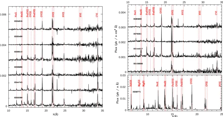
Figure 1 shows the high-resolution spectra of our targets. Lines from H-like and He-like ions of C, N, O, Ne, Mg, and Si, along with lines from ionised Fe, are readily detected, demonstrating the thermal nature of the X-ray emissions. In general, the triplet from He-like ions appear stronger than Lyα lines, as expected for late-type massive stars (Walborn et al. 2009), but we find no clear, systematic dependence with the spectral types of our tar-gets.
An examination of the line profiles reveals no obvious asym-metry, hence we decided to fit them by simple Gaussian profiles. We relied on Cash statistics and therefore used unbinned spec-tra without background correction. We only fitted the lines that were sufficiently intense to provide a meaningful fit. In case of doublets (the two components of Lyman lines of H-like ions) or triplets (the f ir components of He-like ions), the individual components were forced to share the same velocity and the same width. Furthermore, the flux ratios between the two Lyman com-ponents and the flux ratios between the two i lines of Si and Mg2
were fixed to the theoretical ratios in ATOMDB3. The derived
line properties are listed in Table 2 with 1σ errors determined us-ing the error command under Xspec. Whenever the fitted width was reaching a null value, a second fitting was performed with the width fixed to zero, and Table 2 provides the results of this second fitting.
2 For N, O, and Ne, the second i component is >30 times less intense, hence can be neglected.
3 See e.g. http://www.atomdb.org/Webguide/webguide.php Article number, page 2 of 15
C az or la & N az é: B sta rs in X -ra ys
Table 1.Journal of the observations and physical properties of the sample stars.
Target name Sp. type d log(LBOL/L⊙) R⋆ Teff NismH ObsID (Rev) Obs. mode PI Start date Flare? Duration
(pc) (R⊙) (K) (1022cm−2) (ks)
HD 34816 (λ Lep) B0.5 V [1] * 261 4.22 4.7 30400 1.66e-2 0690200601 (2415) ff+thick Nazé 2013-02-15@07:41:26 N 26.5
HD 35468 (γ Ori) B2 IV–III [2] * 77 3.87 6.4 21250 1.82e-3 0690680501 (2342) ff+thick Waldron 2012-09-22@19:27:17 Y 42.0
HD 36512 (υ Ori) B0 V [1] * 877 5.21 12.1 33400 1.95e-2 0690200201 (2326) ff+thick Nazé 2012-08-22@02:46:15 Y 20.2
HD 36960 B0.7 V [1] * 495 4.58 7.8 29000 2.24e-2 0690200501 (2433) ff+thick Nazé 2013-03-23@08:57:52 Y 28.2
HD 38771 (κ Ori) B0.5 Ia [3] 198 4.72 12.5 24800 3.39e-2 9940 ACIS-S Waldron 2008-12-26@23:50:00 234.2
10846 +HETG, 2008-12-30@02:53:17
9939 faint 2009-01-03@03:00:24
10839 2009-01-05@18:25:49
HD 44743 (β CMa) B1 II–III [4] 151 4.41 8.8 24700 2.00e-4 0503500101 (1509) ff+thick Waldron 2008-03-06@15:33:36 Y 10.6
0761090101 (2814) ff+thick Oskinova 2015-04-21@06:44:53 Y 78.0
HD 52089 (ǫ CMa) B1.5 II [4] 124 4.35 9.9 22500 1.00e-4 0069750101 (0234)ff(MOS)/sw(pn)+thick Cohen 2001-03-19@12:05:51 Y 31.2
HD 63922 (P Pup) B0.2 III+? [1,5] * 505 4.95 10.4 31200 6.71e-2 0720390601 (2552) ff+thick Nazé 2013-11-15@02:11:45 N 46.5
HD 79351 (a Car) B2.5 V+? [6,7] * 137 3.60 5.8 19150 6.04e-2 0690200701 (2393) ff+thick Nazé 2013-01-02@00:12:30 N 47.1
HD 144217 (β1Sco) B0.5IV-V+B1.5V [8] * 124 4.44 6.1 30400 1.37e-1 0690200301 (2425) ff+thick Nazé 2013-03-06@16:04:28 N 26.6
HD 158926 (λ Sco) B1.5 IV+ (DA.79
or PMS)+B [9,10] * 175 4.73 15.3 22500 2.51e-3 0690200101 (2424) ff+thick Nazé 2013-03-04@15:37:29 N 17.8
Notes. References for spectral types: [1] Nieva (2013); [2] Morel et al. (2008); [3] Lennon et al. (1992); [4] Fossati et al. (2015); [5] Nieva & Przybilla (2014); [6] Slettebak (1982); [7] Buscombe & Morris (1960); [8] Holmgren et al. (1997); [9] Holberg et al. (2013); [10] Uytterhoeven et al. (2004a). Distances, based on Hipparcos, come from van Leeuwen (2007) and inter-stellar absorbing columns Nism
H were taken from Table 2 (the most recent values) of Gudennavar et al. (2012), except for HD 36960 (for which there is no available value in Gudennavar et al. 2012
so the adopted value is taken from Diplas & Savage 1994) and HD 63922, for which only the colour excess is known (E(B − V) = 0.11; Katyal et al. 2013), which was converted into an absorbing column using the relation of Gudennavar et al. (2012). Bolometric luminosities (for the primary star if binary) were calculated using their Simbad V magnitudes, Hipparcos distances, reddenings from Gudennavar et al. (2012, except for HD 63922, see above), and bolometric corrections of Nieva (2013) for non-supergiant stars (identified by *) and the scale of Cox (2002) for HD 38771. Effective temperatures Teffwere also taken from the latter two references with the addition of Fossati et al. (2015) for HD 44743 and HD 52089 (these authors also provided LBOLvalues for those
stars, which are quoted in a previous column). Radii were calculated from LBOL=4 π R2⋆σ Teff4. For the EPIC cameras, “ff” and “sw” correspond to full frame and small window modes, respectively;
the thick filter was always needed to reject optical/UV light in view of the (optical/UV) brightness of the targets. The durations in the last column correspond to exposure times after flare filtering for EPIC-pn or ACIS-S (0th order). The κ Ori data, taken within 10 days, were combined, so that only the total duration is provided.
A rti cle nu m be r, pa ge 3 of 15
A & A pr oo fs: m an us cri pt no .p ap er
Table 2.Results of the individual line fitting by Gaussians.
HD 34816 HD 35468 HD 36512 HD 36960 HD 38771 HD 44743 HD 52089 HD 63922 HD 79351 HD 144217 HD 158926 He-like triplets Si xiii λ6.648,6.685,6.688,6.740Å v(km s−1) 136±90 FW H M(km s−1) 1201±182 Fr 2.72±0.33 Fi 0.62±0.19 Ff 1.29±0.23 f /i 2.08±0.74 ( f + i)/r 0.70±0.14 Tf ir(keV) 1.30±0.81 Mg xi λ9.169,9.228,9.231,9.314Å v(km s−1) –34±57 FW H M(km s−1) 1132±108 Fr 5.45±0.55 Fi 3.00±0.48 Ff 2.87±0.45 f /i 0.96±0.21 ( f + i)/r 1.08±0.16 Tf ir(keV) 0.25±0.08 Rf ir(R⋆) 2.38±0.44 Ne ix λ13.447,13.553,13.699Å v(km s−1) –160±67 –54±44 –95±110 24±130 –54±109 –37±86 FW H M(km s−1) 0 (fixed) 1310±71 732±309 830±291 369±441 0 (fixed) Fr 22.9±4.5 50.1±3.0 17.3±2.4 33.8±4.6 17.5±2.5 38.0±7.4 Fi 26.7±4.7 31.7±2.9 11.2±2.2 19.5±4.2 12.1±2.4 41.5±8.4 Ff 6.53±3.38 7.97±1.62 3.28±1.47 0.46±2.59 5.56±1.89 4.36±4.56 O vii λ21.602,21.804,22.098Å v(km s−1) 1±146 142±111 0±57 –254±98 –2±47 –31±31 0±60 79±61 –135±61 0±108
FW H M(km s−1) 0 (fixed) 0 (fixed) 361±353 313±406 1353±80 426±198 0 (fixed) 1033±144 0 (fixed) 845±391
Fr 66.0±8.3 18.7±4.1 161±17 44.1±9.9 300±27 84.5±6.8 107±8 102±8 204±19 82.9±10.0 Fi 73.1±8.6 28.8±4.7 175±20 53.8±10.3 238±24 107±7 117±9 90.6±7.9 210±20 57.2±9.9 Ff 2.87±3.95 0 (fixed) 3.08±6.03 0.20±4.65 25.2±10.3 0.±0.73 6.80±3.95 1.18±3.13 4.59±6.96 8.65±5.94 f /i 0.04±0.05 0 (fixed) 0.02±0.03 0.0±0.09 0.11±0.04 0.000±0.007 0.06±0.03 0.01±0.03 0.02±0.03 0.15±0.11 ( f + i)/r 1.15±0.20 1.55±0.42 1.11±0.17 1.22±0.38 0.88±0.12 1.26±0.13 1.16±0.13 0.90±0.11 1.05±0.14 0.79±0.17 Tf ir(keV) 0.09±0.05 <0.09 0.10±0.03 0.09±0.08 0.22±0.08 <0.09 0.09±0.03 0.18±0.06 0.12±0.05 0.26±0.18 Rf ir(R⋆) <10.1 <8.3 <9.8 7.4±2.3 <2.1 4.5±2.4 <6.9 <7.6 7.3±6.5 N vi λ28.787,29.084,29.535Å v(km s−1) –127±76 FW H M(km s−1) 685±182 Fr 42.8±5.9 Fi 49.3±9.2 Ff 0.0±3.1 f /i 0.00±0.06 ( f + i)/r 1.15±0.28 Tf ir(keV) 0.09±0.08 Rf ir(R⋆) <3.7 A rti cle nu m be r, pa ge 4 of 15
C az or la & N az é: B sta rs in X -ra ys Table 2.Continued HD 34816 HD 35468 HD 36512 HD 36960 HD 38771 HD 44743 HD 52089 HD 63922 HD 79351 HD 144217 HD 158926 Lyman doublets Mg xii λ8.419,8.425Å v(km s−1) –222±200 FW H M(km s−1) 1046±475 F 0.91±0.21 He-to-H ratio 12.5±3.1 THe/H(keV) 0.42±0.02 Ne x λ12.132,12.137Å v(km s−1) 1±314 –72±43 1±147 4±192 283±80
FW H M(km s−1) 1111±836 1037±93 0 (fixed) 0 (fixed) 0 (fixed)
F 24.9±4.1 19.4±1.3 13.4±1.7 25.8±3.1 18.5±2.7
O viii Lyα λ18.967,18.973Å
v(km s−1) –2±69 144±379 0±31 –292±194 –144±36 0±27 –33±33 27±53 112±120 –87±41 –127±156
FW H M(km s−1) 583±322 1750±1750 0 (fixed) 0 (fixed) 1267±69 0 (fixed) 283±247 709±190 0 (fixed) 0 (fixed) 760±759
F 57.1±4.2 12.3±2.2 126±8 42.2±5.4 261±11 97.0±3.2 159±5 109±5 22.4±3.2 218±13 32.4±4.2
He-to-H ratio 2.49±0.28 3.85±0.85 2.69±0.27 2.33±0.47 2.16±0.17 1.97±0.12 1.45±0.09 1.78±0.14 1.92±0.17 4.59±0.76
THe/H(keV) 0.193±0.004 0.18±0.01 0.189±0.004 0.19±0.01 0.198±0.004 0.207±0.004 0.22±0.01 0.202±0.005 0.189±0.004 0.168±0.004
O viii Lyβ λ16.006,16.007Å
v(km s−1) –228±152 –130±145 0±279 160±60 84±206 –171±171
FW H M(km s−1) 0 (fixed) 1296±159 1087±429 0 (fixed) 933±602 0 (fixed)
F 14.7±3.6 34.0±3.3 11.3±1.8 26.0±3.4 14.4±2.5 34.0±4.5 N vii λ24.779,24.785Å v(km s−1) –73±133 –299±107 92±131 2±123 85±83 –4±118 FW H M(km s−1) 439±495 0 (fixed) 1838±233 0 (fixed) 1264±254 729±535 F 23.4±4.8 37.2±8.2 158±15 19.5±2.7 72.0±5.9 24.8±4.4 He-to-H ratio 1.28±0.19 THe/H(keV) 0.15±0.01 C vi λ33.734,33.740Å v(km s−1) 64±86 0±60 –122±49 122±91 FW H M(km s−1) 470±469 268±267 328±328 0 (fixed) F 127±17 84.1±8.1 91.1±8.4 79.9±13.6 Fe xvii λ15.014,15.261Å v(km s−1) 1±50 –115±36 9±49 0±56 188±130 0±65 104±166
FW H M(km s−1) 0 (fixed) 1192±81 707±185 0 (fixed) 927±477 0 (fixed) 1385±482
F 38.7±5.2 96.2±4.4 51.6±2.5 112±5 33.0±3.4 26.4±2.8 84.5±8.2
Fe xvii λ16.780,17.051,17.096Å
v(km s−1) –373±154 –585±42 –474±58 –602±26 –490±86 –614±147 –665±56
FW H M(km s−1) 937±632 989±90 0 (fixed) 0 (fixed) 504±504 0 (fixed) 0 (fixed)
F16.780 17.1±3.9 40.2±4.2 18.8±1.9 40.3±3.5 8.28±2.07 5.42±2.03 21.6±4.9
Fboth17 54.1±8.1 107±6 49.4±3.0 115±5 33.7±3.3 27.7±3.0 79.7±8.1
Notes.Fluxes are given in units 10−6ph cm−2s−1, and correspond to fluxes for all components of Lyman doublets or of iron line groups. The provided ratios are uncorrected for interstellar absorption; since the f flux of O vii was set to zero for HD 35468, no Rf irwas derived in this case. For the He-like triplet of Neon, the presence of multiple iron lines in the area may render the line fluxes unreliable because of blending with iron lines, hence they are provided for information only and the ratios are not indicated. Errors correspond to 1σ uncertainties – if asymmetric, the larger value is given here. A rti cle nu m be r, pa ge 5 of 15
A&A proofs: manuscript no. paper 10 15 20 25 30 35 0 0.002 0.004 0.006 10 15 20 25 30 35 0 0.001 0.002 0.003 0.004 10 15 20 25 0 0.01 0.02 0.03
Fig. 1.RGS and MEG spectra of our targets with the main lines identified and their position indicated by the dotted lines. We compared the results obtained for the different lines for
each target, taking the errors4 into account but we detected no
significant (> 3σ) and coherent line shifts for any of them. There are systematic blueshifts for the iron lines near 17Å for all tar-gets, which remain unexplained and are probably not real. Ex-cluding these blueshifts, we find that 59% of measurements lie within ±1σ of zero, 83% lie within ±2σ, and 97% lie within ±3σ; these measurements match well the normal distribution centred on zero. Our targets hence display no line shifts. Sim-ilarly, the line widths appear overall negligible compared to the resolution for all targets except HD 38771, for which FWHM ∼ 1250 km s−1, which is a value close to the wind terminal velocity
(Crowther et al. 2006; Searle et al. 2008). While other stars were observed using the RGS, which has a poorer spectral resolution than HEG/MEG, it should be noted that FWHM larger than 1000 km s−1 would have been detected, considering the errors
and instrumental broadening. The X-ray lines thus generally ap-pear quite narrow, confirming the results found for other B stars (e.g. Waldron & Cassinelli 2007; Cohen et al. 2008; Favata et al. 2009).
We now turn to the line ratios: ( f + i)/r in He-like triplets and flux ratios between He-like and H-like lines are indicators of temperature while R = f /i is a probe of the formation radius of the X-ray emission. Correcting for the energy-dependent inter-stellar absorption is unnecessary for ratios involving the closely spaced f ir lines, but such a correction needs to be performed for the He-to-H-like flux ratios since the lines are more distant in this case. However, since our targets are nearby, their interstellar absorptions are small (Table 1), hence these corrections are of very limited amplitude.
4 The errors on shifts in Table 2 were derived from fitting errors and er-ror propagation, hence systematic uncertainties are not included. While those linked to atomic parameters (ATOMDB) are difficult to estimate, it is known that, for example the RGS wavelength scale displays vari-ations with σ ∼ 5 mÅ (de Vries et al. 2015), corresponding to an addi-tional error of 70–80 km s−1on the positions of the oxygen lines.
As in Nazé et al. (2012), we used the ATOMDB, although with the newer version 3.0.8, to compute the expected ratios He-to-H-like flux ratios and ( f + i)/r ratios as a function of temper-atures, and compared them to the observed values (see results in Table 2). The derived temperatures, typically log(T ) ∼ 6.35, are in line with the lowest ones found in global fits (see next section) and are also comparable to temperatures observed in normal B stars (e.g. Waldron & Cassinelli 2007; Zhekov & Palla 2007, see also further below).
The negligible f lines indicate that the emission from He-like triplets arises close to a source of UV, i.e. close to the stellar photosphere (e.g. Porquet et al. 2001). In fact, for massive stars, R = f /i = R0/(1 + φ/φC). The R0 values were derived from
ATOMDB calculations, and taken at the temperature indicated by the ( f +i)/r ratio (see above and Table 2). The φCvalues were
taken from Blumenthal et al. (1972). Finally, we used TLUSTY spectra (Lanz & Hubeny 2003, 2007) in the UV domain with solar abundances to get the stellar fluxes in the velocity inter-val [–2000; 0] km s−1 near the rest wavelengths of the 23S
1→
23P
1,2 transition (for a similar approach, see Leutenegger et al.
2006). We consider TLUSTY models with the closest tem-peratures to the ones listed in Table 1 and the closest sur-face gravities predicted by Nieva (2013) for the different spec-tral types of non-supergiant stars – for HD 38771, HD 44743, and HD 52089, the surface gravities derived by Touhami et al. (2010) and Fossati et al. (2015) were considered. A microtur-bulence velocity of ξ=10 km s−1, which is a value adapted to
our target types (e.g. Hunter et al. 2009), was considered, un-less models with the required temperatures and surface gravi-ties were not available within the TLUSTY grid associated to ξ=10 km s−1 (i.e. for HD 35468, HD 44743, HD 52089, and
HD 158926). In this case, TLUSTY models with ξ=2 km s−1
were taken into account. We performed tests to check the con-sistency of our choice: using these two microturbulence veloc-ities resulted in similar formation radii, within error bars, for an effective temperature of 22000 K and a surface gravity of Article number, page 6 of 15
Cazorla & Nazé: B stars in X-rays 3.00 dex. Since these UV fluxes are diluted for calculating the
φvalues, which can be represented by the multiplication by the dilution factor W(r) = 0.5 {1 − [1 − (R⋆/r)2]1/2}, the R ratios
constrain the position of the emitting plasma (see Rf ir in Table 2). Note that UV TLUSTY spectra only cover the 900 – 3200 Å wavelength range, which therefore excludes the analysis of the Si xiii triplet lines, hence Rf ir is not indicated in that case, but this concerned only HD 38771 (and its f /i ratio is very sim-ilar to that reported for HD 37128, HD 111123, or HD 149438 by Waldron & Cassinelli 2007). Focusing on the formation radii derived from O vii lines (since they are available for all but one star), values ranging from ∼ 2 to ∼ 8 R⋆ are found. This is
in good agreement with values determined for the same lines for the studied B stars mentioned in Sect. 2: for HD 205021, Favata et al. (2009) derived a formation radius in the range ≃ 3 – 5 R⋆; for HD 122451, Raassen et al. (2005) estimated a
for-mation radius . 5.7 R⋆; Nazé & Rauw (2008) gave a formation
radius < 20 R⋆ for HD 93030; Miller (2007) derived a
forma-tion radius in the range 5 – 8 R⋆ for HD 116658; Mewe et al.
(2003) estimated the formation radius of HD 149438 to be . 10 R⋆; for HD 37128, Waldron & Cassinelli (2007) provided a
for-mation radius of 10.2±2.6 R⋆.
3.2. Global fits
Having both low-resolution, broadband spectra (EPIC, ACIS-S 0th order) and high-resolution, narrower band spectra (RGACIS-S, HEG/MEG) allows us to investigate the full X-ray spectra in detail, deriving not only temperatures and absorptions, but also abundances. However, caution must be taken since abundances may vary wildly when all parameters are relaxed in one step. Therefore, we performed global fits in several steps. First, we fitted the low-resolution spectra with absorbed thermal emission models with fixed solar abundances (Asplund et al. 2009). One thermal component was never sufficient to achieve a good fit, but two components were usually adequate, except for HD 36960, HD 79351, and HD 144217, for which three components were needed to fit a high-energy tail. Fits with absorption in addition to the interstellar one were tried, but either the additional ab-sorbing column reached a null value or the χ2 was worse than
without such a column. This absence of (detectable) local ab-sorption is usual for B stars (Nazé et al. 2011; Rauw et al. 2015) and for the final fits we therefore considered only the interstel-lar contributions (see Table 1 for their values). Second, we fit-ted the high-resolution spectra with the same thermal models, but we fixed the temperatures while releasing abundances. The abundance of an element is only allowed to vary if lines of that element are clearly observed (and measured, see Table 2). In the third step, the temperatures were released again for fitting the high-resolution spectra. Finally, in the fourth step, a simulta-neous fitting of both low-resolution and high-resolution spectra was performed with the same model as in the third step. The fi-nal results are provided in Table 3. The abundances found in the last two steps are similar, but they sometimes differ from those found in the second step, indicating that the formal error bars might actually be underestimated.
In general, the X-ray spectra appear very soft and the as-sociated temperatures are low, i.e. 0.2–0.6 keV, in line with results from Raassen et al. (2005); Zhekov & Palla (2007); Nazé & Rauw (2008); Gorski & Ignace (2010) for optically bright, nearby B stars observed at high resolution in X-rays. However, in large surveys relying on low-resolution X-ray spec-tra, many B stars present higher temperatures (Nazé 2009;
Nazé et al. 2011), although the contamination by companions or magnetically confined winds cannot be excluded in such cases. In our sample, only three targets appear harder with a hotter component, i.e. HD 36960, HD 79351, and HD 144217. The last two are binaries and we may suspect that this plays a role in their properties. However, only longer observations including full monitoring throughout the orbital period, would be able to reveal the exact origin of the hard X-rays, which could be emit-ted by the companion or result from an interaction with it. For HD 36960, however, there is no obvious reason for such a hard-ness: it is not a known binary or magnetic object. Further inves-tigation is thus needed to clarify this issue.
The X-ray luminosities of massive stars are generally com-pared to their bolometric luminosities (see penultimate line of Table 3). For single and non-magnetic O-type stars in clus-ters, the ratio log(LX/LBOL) is close to −7 with a dispersion
of about 0.2 dex (e.g. Nazé et al. 2011). The situation appears more complex for early B stars. Surveys show a large scatter with ratios between –8 and –6 and the X-ray emission often appears at a constant flux level for the (rather few) detected cases (Berghöfer et al. 1996; Nazé et al. 2011, 2014; Rauw et al. 2015); again, contamination of the X-ray emission by compan-ions cannot be excluded. Furthermore, while magnetic O stars systematically appear brighter than their non-magnetic counter-parts, this is not the case of magnetic B stars (log [LX/LBOL] ∼
−7.6 for the faintest case in Fig. 4 and Table 7 of Nazé et al. 2014), which further blurs the picture. However, our sample is rather clean in this respect, as the chosen B stars are nearby and not strongly magnetic (see Sect. 2). Our earliest B-type stars (B0–0.7) display ratios between –6.8 and –7.4, in line with the O-star relationship. This confirms previous results for such ob-jects (Rauw et al. 2015, and references therein). Four of the five latest B-type stars (B1–2.5) have ratios < −7.4, confirming the lower level of intrinsic X-ray emission of such (non-magnetic) stars found in ROSAT data (Cohen et al. 1997) and attributed to their weakest stellar winds. However, the last star, HD 79351, appears overluminous. This can probably be explained by its bi-narity; in this context, it is interesting to note that a flare occurred during the observation of this star (see next section).
In massive stars, X-rays are linked to stellar winds. The amount of X-ray emission can therefore be used to estimate the amount of mass loss heated to high temperatures. This is im-portant information since, in the tenuous winds of B stars and late O stars, cooling times are long and hence the plasma re-mains hot once heated. Estimating mass-loss rates from opti-cal/UV diagnostics may thus lead to underestimations. This was clearly demonstrated by Huenemoerder et al. (2012) for the late O star HD 38666 (see also a similar discussion for HD 111123 in Cohen et al. 2008). We have used the best-fit normalisation factors (Table 3) to calculate the total emission measures EMs (since norm = 10−14E M/[4 π d2]), summing those of individual
components (Table 4). These values were converted into rates of hot mass loss considering Eq. 1 of Huenemoerder et al. (2012) and its equivalent for constant velocity on p. 1868 of Cohen et al. (2008, correcting by the different stellar radii of our targets). This was carried out considering terminal wind velocities of 500, 1000, and 1500 km s−1 and the formation radius derived
for O vii lines (Table 2). The derived range of values are pro-vided in Table 4. We also computed mass-loss rates from the formulae of Vink et al. (2001, listed in Table 4), using the tem-perature and bolometric luminosities of our targets listed in Ta-ble 1, along with typical masses for the spectral types of our targets, taken from Cox (2002). Finally, mass-loss estimates de-rived from the analysis of optical spectra are also provided in Article number, page 7 of 15
A & A pr oo fs: m an us cri pt no .p ap er
Table 3.Results of the global fitting using models of the type tbabs(ism) × P vapeci.
HD 34816 HD 35468 HD 36512 HD 36960 HD 38771∗ HD 44743 HD 52089 HD 63922 HD 79351 HD 144217 HD 158926 kT1 0.186±0.004 0.172±0.004 0.116±0.008 0.081±0.001 0.215±0.010 0.197±0.001 0.199±0.002 0.190±0.002 0.223±0.016 0.188±0.003 0.174±0.006 norm1 8.63±0.42 2.91±0.10 19.8±3.7 13.6±0.78 46.5±4.3 7.66±0.28 9.93±0.40 13.3±0.5 4.07±0.23 27.6±1.21 5.37±0.40 kT2 0.41±0.07 0.59±0.03 0.291±0.004 0.459±0.015 0.52±0.02 0.558±0.006 0.579±0.004 0.488±0.017 0.74±0.02 0.481±0.019 0.48±0.06 norm2 0.46±0.30 0.19±0.02 7.00±0.55 1.20±0.04 7.30±0.82 1.91±0.05 5.78±0.13 1.78±0.13 3.73±0.09 4.18±0.35 0.43±0.09 kT3 2.50±0.08 1.60±0.03 4.4±6.2 norm3 2.85±0.07 3.73±0.09 0.32±0.10 χ2ν(dof) 1.39(454) 1.04(463) 1.31 (476) 1.35 (463) 1.08 (521) 1.54 (1414) 1.44 (1139) 1.21 (798) 1.40 (1020) 1.20 (377) 1.12 (312) AC 0.61±0.16 1.69±0.16 1.26±0.13 1.61±0.35 AN 1.07±0.13 1.03±0.17 1.05±0.33 1.27±0.09 2.28±0.15 1.21±0.11 AO 0.54±0.03 0.45±0.03 0.97±0.11 2.74±0.15 0.33±0.03 0.78±0.03 0.76±0.03 0.69±0.03 0.34±0.03 0.78±0.04 0.74±0.07 AN/AC 1.69±0.52 0.75±0.09 1.81±0.22 AN/AO 1.98±0.26 1.06±0.21 3.18±1.04 1.62±0.13 3.00±0.23 1.75±0.18 ANe 1.41±0.12 5.40±0.32 0.65±0.07 1.79±0.08 1.67±0.07 1.29±0.06 1.99±0.42 1.73±0.10 AFe 0.83±0.06 0.40±0.04 1.00±0.03 0.85±0.02 0.87±0.04 0.78±0.04 0.93±0.06 AO/AFe 1.17±0.16 0.83±0.11 0.78±0.04 0.89±0.04 0.79±0.05 0.44±0.04 0.84±0.07 FobsX 0.42±0.02 0.135±0.003 1.08±0.03 0.83±0.06 2.10±0.06 0.926±0.005 1.80±0.01 0.788±0.006 1.037±0.007 1.47±0.02 0.343±0.010 log(LX/LBOL) −7.24 ± 0.02 −8.48 ± 0.01 −6.77 ± 0.01 −6.76 ± 0.03 −7.26 ± 0.01 −7.597 ± 0.002 −7.421 ± 0.002 −7.044 ± 0.003 −6.767 ± 0.003 −7.38 ± 0.01 −8.21 ± 0.01 eq. ROSAT c.r. 0.134 0.095 0.397 0.176 0.326 0.341 0.537 0.091 0.102 0.142 0.178
Notes.Temperatures are in keV, normalisation factors in 10−4cm−5, fluxes in the 0.5–10.0 keV energy band in 10−12erg cm−2s−1, abundances Aiin number, with respect to hydrogen, and with respect to solar values (Asplund et al. 2009). Errors, derived from the Xspec error command for parameters and from flux err for fluxes, correspond to 1σ uncertainties – if asymmetric, the larger value is given here. EPIC spectra were fitted above 0.25 keV and ACIS-S 0th order spectra above 0.35 keV.
∗For HD 38771, there are three additional parameters: A
Mg=0.44±0.06, AS i=0.52±0.08, and the Gaussian smoothing (gsmooth, convolved to the thermal model) with σ = (1.23±0.05)×10−3keV at 6 keV, corresponding to FWHM = 145 ± 6 km s−1. This smaller value, compared to individual line fits, may be explained by the grouping used for global fits, which blurs the line profiles.
A rti cle nu m be r, pa ge 8 of 15
Cazorla & Nazé: B stars in X-rays Table 4, when available. Comparing all these values, we find
that our targets fall into two categories. The hot plasma consti-tutes a small (or even negligible) part of the wind for HD 36512, HD 38771, HD 44743, HD 63922, and HD 158926, or about half of the sample. For the other stars, the hot plasma appears as the dominant component of the circumstellar environment, as in HD 38666 (Huenemoerder et al. 2012). In examining which stel-lar properties could justify this dichotomy, we find variable stars (see next section) and binaries in both categories; hence variabil-ity or multiplicvariabil-ity are not specific characteristics of stellar winds dominated by hot plasma. However, the three stars displaying a very hot component in their X-ray spectrum all belong to the second category, i.e. stars whose winds appear to be dominated by hot plasma. For such stars, the EM may not perfectly reflect the intrinsic X-ray emission as there may be contamination by X-rays arising in a companion, in an interaction with it, or a still unknown phenomenon (see above). Further investigation is thus needed to ascertain that most of their wind truly is hot. In any case, our analysis suggests that some B stars have their winds in the X-ray emitting regime, such that using only optical/UV data could lead to underestimation of their actual mass-loss rate. We caution, however, that this result is preliminary, as detailed anal-ysis of the optical/UV spectra are often not available for those stars.
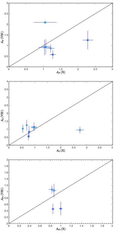
The abundances of our sample stars derived from our X-ray fits are listed in Table 3 and those determined in optical studies from the literature are listed in Table 5. Figure 2 pro-vides a graphical comparison for the main elements (N, O, and Fe) for the stars in common. Except for the high O enrich-ment derived in X-rays for HD 36960, which is not confirmed in the optical domain, the agreement between the derived abun-dances is fair (generally well within 3σ). Indeed, the formal fit errors are known to be smaller than the actual fit errors (e.g. de Plaa et al. 2017). An example of disagreement can also be found in the subsolar abundances found by Cohen et al. (2008) and Zhekov & Palla (2007) for HD 111123: even though they analysed the same dataset, the Zhekov & Palla (2007) abun-dances of O, Ne, and Mg are a factor of two smaller than those of Cohen et al. (2008); the origin of this discrepancy is unknown. We also note disagreements between optical studies, for example for HD 38771 or HD 52089, showing that improvements are re-quired there too. In any case, not many comparisons between X-ray and optical abundances can be found in the literature. For HD 205021, Favata et al. (2009) derived O, Si, and Fe abun-dances that are depleted compared to photospheric abunabun-dances. Nazé & Rauw (2008) confirmed the depletion in C and O of HD 93030 as well as its enrichment in N reported in the op-tical domain by Hubrig et al. (2008). In fact, X-ray determina-tions would benefit from higher S/N data; for example, the X-ray abundances of HD 66811, derived from very high-quality spec-tra, could be better constrained (Hervé et al. 2013).
4. Light curves
We finally examined the temporal evolution of the X-ray bright-nesses of our targets. The light curves in the 0.3–10. keV en-ergy band are shown in Fig. 3. We first performed χ2 tests for
three different null hypotheses (constancy, linear variation, and quadratic variation). The improvement of the χ2when increasing
the number of parameters in the model (e.g. linear trend versus constancy) was also determined by means of Snedecor F tests (nested models; see Sect. 12.2.5 in Lindgren 1976). As threshold for significance, we used 1% and we considered that a threshold
Fig. 2.Comparison between our N (upper panel), O (middle panel), and Fe (lower panel) abundance estimates and recent literature val-ues obtained by optical studies. Circles, triangles, diamonds, squares, and star symbols represent values obtained by Nieva & Przybilla (2012), Venn et al. (2002), Valdes et al. (2004), Searle et al. (2008), and Morel et al. (2006, 2008), respectively.
of 10% indicates only marginal evidence. This yields the follow-ing results.
Two stars are clearly compatible with constancy, i.e. HD 34816 and HD 38771. For the latter, only the ACIS-S light curve with 1ks bins could be analysed, as there are not enough counts in each bin for a meaningful χ2 test of the 100s-binned
light curves. We also analysed the light curves of each Chandra exposure with the appropriate CIAO tool5, and the variability
5 http://cxc.harvard.edu/ciao/threads/variable/index.html#glvary Article number, page 9 of 15
A & A pr oo fs: m an us cri pt no .p ap er
Table 4.Derived mass loss from optical studies and estimates, from different prescriptions, of the hot mass loss derived with our X-ray data.
Target name log( ˙Mliterature) log( ˙MVink+01) E M log( ˙MHuenemoerder+12) log( ˙MCohen+08)
(M⊙yr−1) (M⊙yr−1) (1052cm−3) (M⊙yr−1) (M⊙yr−1)
Low Teff High Teff
HD 34816 −8.50±0.06 74.1±4.2 <–8.1 to <–7.6 <–8.0 to <–7.6 HD 35468 −8.33±0.09 2.20±0.07 –10.0 to –8.4a –9.3 to –8.4a HD 36512 −6.22±0.06 2466±344 <–7.2 to <–6.7 <–7.1 to <–6.6 HD 36960 −7.79±0.07 159±23 <–7.8 to <–7.3 <–7.8 to <–7.3 HD 38771 −6.05 [1], −5.92+0.11 −0.07[2] −6.80±0.08 −8.01±0.07 252±21 –7.7 to –7.2 –7.6 to –7.2 HD 44743 −7.33±0.08 −8.55±0.08 26.1±0.8 <–8.6 to <–8.2 <–8.5 to <–8.0 HD 52089 −9 [3],−8 [4] −7.53±0.08 28.9±0.8 –8.3 to –7.8 –8.3 to –7.8 HD 63922 −6.93±0.06 460±16 <–7.6 to <–7.1 <–7.6 to <–7.1 HD 79351 −8.71±0.10 25.9±0.6 –9.5 to –7.9a –8.7 to –7.8a HD 144217 −8.04±0.06 59.1±2.3 <–8.1 to <–7.7 <–8.1 to <–7.6 HD 158926 −6.50±0.08 19.8±1.5 –8.2 to –7.7 –8.1 to –7.7
Notes.The second column lists the mass-loss rate value derived in recent optical studies using atmosphere models: [1]: Crowther et al. (2006), [2]: Searle et al. (2008), [3]: Hamann et al. (priv. comm. with Fossati et al. 2015), [4]: Najarro et al. (1996). The third and fourth columns provide the mass-loss estimates from the formulae of Vink et al. (2001) when the adopted Teff is in the
range 12500 – 22500 K (cool side of the bi-stability jump) and 27500 − 50000 K (hot side of the bi-stability jump), respectively. When the adopted Teff(Table 1) is in the range 22500 − 27500 K
(in the bi-stability jump), mass-loss estimates for both the cool and hot sides of the bi-stability jump are provided. The fifth column yields the total X-ray emission measures, estimated from the normalisation factors of the spectral fittings (Table 3). The last two columns provide the mass-loss rates predicted by Eq. 1 of Huenemoerder et al. (2012, with b=0.97) and the formula on p. 1868 of Cohen et al. (2008), respectively. In these columns only a range of mass-loss rates are given: the lower values correspond to a terminal wind velocity of 500 km s−1, while the highest values
correspond to a terminal wind velocity of 1500 km s−1.a: These values were derived assuming R
f ir=1 to 7 R⋆, which is in line with the formation radii derived in Sect. 3.1.
A rti cle nu m be r, pa ge 10 of 15
C az or la & N az é: B sta rs in X -ra ys
Table 5.Stellar abundances from optical studies.
HD 34816 HD 35468 HD 36512 HD 36960 HD 38771 AC 0.68 [1], 0.89±0.15 [2] 0.71 [3], 0.74 [1] 0.83±0.28 [2], 0.85±0.31 [7], 0.89±0.31 [6] 0.74±0.18 [9], 0.83±0.20 [2] 0.11 [10], 0.20 [11] AN 0.68 [1], 0.95±0.35 [2] 1.82 [3], 2.00 [1] 0.89±0.31 [6], 0.91±0.36 [2], 1.00±0.26 [7] 0.76±0.16 [9], 0.78±0.22 [2] 0.35±0.13, 2.69±0.92 [10], 2.09 [11] AO 1.04±0.25 [2], 1.15 [1] 1.05±0.34 [8], 1.06±0.41 [6], 1.15±0.27 [2] 0.95±0.21 [2], 1.07±0.21 [9] 1.10 [11], 1.29±0.38 [10] AN/AC 1.00 [1], 1.07±0.43 [2] 2.56 [3], 2.70 [1] 1.10±0.57 [2], 1.00±0.49 [6], 1.18±0.53 [7] 0.94±0.35 [2], 1.03±0.33 [9] 3.18±1.18;24.5±8.4 [10], 10.45 [11] AN/AO 0.59 [1], 0.91±0.40 [2] 0.84±0.44 [6], 0.79±0.36 [2] 0.71±0.20 [9], 0.82±0.39 [2] 0.27±0.13;2.09±0.94 [10], 1.90 [11] ANe 1.77±0.16 [2] 1.12±0.26 [4] 1.52±0.43 [2], 1.70±0.55 [7] 1.59±0.54 [2] AFe 1.10±0.20 [2] 0.83 [5] 1.07±0.12 [2], 1.12±0.12 [7] 0.96±0.22 [2] AO/AFe 0.95±0.28 [2] 1.07±0.28 [2] 0.99±0.32 [2] AMg 0.40 [10] AS i 0.45 [10] HD 44743 HD 52089 HD 63922 AC 0.54±0.15 [12], 0.60 [1], 0.63 [3], 0.78±0.20 [14] 0.46±0.14 [12], 0.74±0.15 [14] 0.74±0.15 [2] AN 0.58±0.20 [12], 0.76 [1], 0.79 [3], 0.83±0.24 [14] 0.81 [15], 1.26±0.43 [12], 2.15±0.42 [14] 0.87±0.19 [2] AO 0.85±0.37 [12], 1.15 [1], 1.23 [3], 1.10±0.28 [14] 0.56±0.24 [12], 1.02±0.30 [14] 1.26±0.32 [2] AN/AC 1.07±0.48 [12], 1.27 [1], 1.25 [3], 1.06±0.41 [14] 2.74±1.25 [12], 2.91±0.82 [14] 1.18±0.35 [2] AN/AO 0.68±0.38 [12], 0.66 [1], 0.64 [3], 0.75±0.29 [14] 2.25±1.23 [12], 2.11±0.74 [14] 0.69±0.23 [2] ANe 0.91±0.34 [4] 0.85±0.24 [4] 1.37±0.39 [2] AFe 0.47±0.21 [13] 0.46±0.16 [12] 1.03±0.21 [2] AO/AFe 1.22±0.67 [12] 1.22±0.40 [2]
Notes.Abundances are in number, with respect to hydrogen, and with respect to solar values, as for the X-ray abundances in Table 3. References: [1] Gies & Lambert (1992), [2] Nieva & Przybilla (2012), [3] Venn et al. (2002), [4] Morel & Butler (2008), [5] Valdes et al. (2004), [6] Martins et al. (2015), [7] Nieva & Simón-Díaz (2011), [8] Simón-Díaz (2010), [9] Kilian (1992), [10] Lennon et al. (1991), [11] Searle et al. (2008), [12] Morel et al. (2008), [13] Morel et al. (2006), [14] Fossati et al. (2015), [15] Fraser et al. (2010).
A rti cle nu m be r, pa ge 11 of 15
A&A proofs: manuscript no. paper index was found to be zero (definitely not variable) for ObsID
9939, 10839, and 10846, and 2 (probably not variable) for Ob-sID 9940, which confirms the χ2results. We also tested the
com-bination of the four individual light curves using χ2tests with the
same null result as for individual light curves.
Four stars reveal marginal variability (i.e. presence of trends and/or rejection of constancy at the 1–10% level), i.e. HD 35468, HD 44743, HD 63922, and HD 144217. HD 35468 is detected to be variable for the MOS2 light curves, but this star is only marginally variable in pn data and appears to be compatible with constancy in MOS1 data. For HD 44743, trends provide better fits for pn data in Rev. 1509 and for MOS1 and pn data for Rev. 2814. A marginal variability is further detected for all instruments in Rev. 2814, and when the two datasets are com-bined. The 100s-bin light curves of HD 144217 are better fitted by trends.
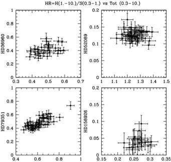
Five stars exhibit a clear variability (significance level <1%), i.e. HD 36512, HD 36960, HD 52089, HD 79351, and HD 158926. HD 36512 is detected to be variable for the 100s-bin pn light curve, and a trend provides a clearly better fit than a constant for MOS2 and pn. HD 36960 appears significantly vari-able for all instruments, with trends – especially parabolic trends – always providing better fits. Indeed, the light curve presents a large oscillation with maxima at the beginning and end of the exposure and a minimum in between. This change in brightness is only marginally accompanied by a change in hardness (see Fig. 4), however. HD 52089 appears variable in pn data and a trend provides a clearly better fit than a constant. HD 79351 ap-pears significantly variable for all instruments. Indeed, the light curve steedily increases at first, then slightly decreases, and fi-nally presents a flare-like activity. Furthermore, when it bright-ens, HD 79351 also becomes harder (see Fig. 4). HD 158926 is detected to be significantly variable for all instruments when considering 100s bins, with trends providing a better fit to pn data.
Next, we applied period search algorithms (Heck et al. 1985; Graham et al. 2013) to the light curves with 100s bins, for each EPIC camera, but no peak stands out both clearly and coherently (i.e. for all instruments) from the periodograms (although see further below).
Two types of specific timescales exist for our tar-gets: orbital periods and pulsation periods. The for-mer are usually long compared to the exposure length (5.9 d for HD 158926, Berghöfer et al. 2000; 6.745 d for HD 79351, Buscombe & Morris 1960; 6.83 d for HD144217, Holmgren et al. 1997), hence cannot be tested with the current dataset. However, we may still examine whether binarity may explain the flare-like behaviour of HD 79351. Indeed, Buscombe & Morris (1960) derived a mass function of 0.00663565 for this system. Assuming the mass taken from Cox (2002, ∼ 10 M⊙) for the primary star, we find a minimum
mass of ∼ 0.7M⊙for the secondary star. It may thus be a PMS
star, which could have undergone a flare during the observation. Indeed, the average X-ray luminosity of HD 79351 is ∼3×1030
erg s−1 (Table 3) and its brightness increased by less than a
factor of 2 during the flare (Fig. 3), which remains compatible with PMS flaring luminosities (Güdel & Nazé 2009). However, a better knowledge of the HD 79351 system is needed before its X-ray properties can be fully understood.
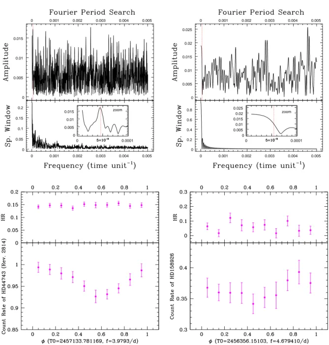
Regarding the latter timescales, it should be noted that the following two targets are known β Cephei: HD 44743 (three closely spaced frequencies with the strongest at f = 3.9793 ± 0.0001 d−1; Shobbrook et al. 2006) and HD 158926 (dominant
frequency at f = 4.679410 ± 0.000013 d−1; Uytterhoeven et al.
2004b). For HD 44743, a peak exists close to that dominant timescale in the periodogram of EPIC data taken in Rev. 2814 (top of Fig. 5). The amplitude of this peak is not very large but it is present and in fact, if the background flares are not discarded hence longer and more complete light curves are available, this peak stands out very clearly. In this context, it should be remem-bered that the known pulsators HD 122451 (β Cen), HD 116658 (Spica), HD 205021 (β Cep), and HD 160578 (κ Sco) do not dis-play X-ray variations linked to their pulsations (Raassen et al. 2005; Miller 2007; Favata et al. 2009; Oskinova et al. 2015), but HD 46328 (ξ1CMa) does (Oskinova et al. 2014; Nazé 2015)
and β Cru may (Cohen et al. 2008, though see refutation in Oskinova et al. 2015). Therefore, even if periodograms do not show very strong peaks at these periods, we performed a fold-ing usfold-ing these known frequencies as a last check (bottom of Fig. 5). For HD 44743, the presence of a modulation is clearly confirmed with a peak-to-peak amplitude of 14% (correspond-ing to five times the error on individual bins); this modulation is not accompanied by significant hardness changes, but neither did HD 46328. The case of HD 158926 appears less convincing as the changes are not coherent from one instrument to the other, and the combination of all three EPIC instruments only leads to a slight modulation (the peak-to-peak variation is only 3σ), clearly calling for confirmation before detection can be claimed. As a final exercise, we folded our best-fit spectral models (Table 3) through the ROSAT response matrices and derived the equivalent ROSAT count rates of our targets (reported in the last line of Table 3). Comparing our results to values tabulated by Berghöfer et al. (1996), we find negligible (< 3σ) differences for all but three targets; HD 35468 and HD 158926 has become fainter by a factor of two, while HD 36512 has brightened by 50%. These three stars thus appear variable on both long and short timescales. While this could probably be linked to bina-rity for HD 158926, there is no clear explanation for the other two. A monitoring of all three stars will then be needed to better understand their behaviour, in particular searching for a putative periodicity.
5. Discussion and conclusions
In this paper, we analysed the X-ray data of 11 early B stars. Combined with 8 other B stars previously analysed, our results provide the first X-ray luminosity-limited survey at high resolu-tion, thereby constituting a legacy project.
In this work, we performed line-by-line fitting, global spec-tral fitting (with temperatures, abundances, and brightnesses as free parameters), and variability analyses.
In many ways, our results confirm previous studies. B stars typically display soft and moderately intense X-ray emissions, their ray lines appear rather narrow and unshifted, and the X-ray emission arises at a few stellar radii from the photospheres.
The abundances we derived are in fair agreement with those found in optical data, taking errors into account. The X-ray brightnesses could be used to evaluate the total quantity of hot material surrounding the stars. Compared to expected mass-loss rates or values derived from the analysis of optical data, we find that in half of the cases, the hot mass-loss constitutes only a small fraction of the wind.
Roughly a quarter of our sample (3/11) display a high-energy tail and roughly half of our targets (6/11) display significant vari-ations on short or long timescales. These properties are not mu-tually exclusive as two targets (HD 36960 and HD 79351) com-bine both specificities. Three out of the four binaries present at Article number, page 12 of 15
Cazorla & Nazé: B stars in X-rays 0 0.2 0.25 0.3 0.35 0.4 0 0.05 0.1 0.15 0.2 0 0.6 0.7 0.8 0.9 1 0 0.3 0.4 0.5 0.6 0.7 0 5000 0.5 0.6 0.7 0.8 0.9
ellapsed time since exposure start (s)
0 0.5 0.6 0.7 0.8 0.9 0 1 1.2 1.4 0 0.4 0.5 0.6 0.7 0 0.4 0.6 0.8 1 0 0.8 0.9 1 1.1 1.2
ellapsed time since exposure start (s)
0 5000 0.15 0.2 0.25 0.3 0.35 0 0.01 0.02 0.03 0.04 0.05 0 0.01 0.02 0.03 0.04 0.05 0 0.01 0.02 0.03 0.04 0.05 0 0.01 0.02 0.03 0.04 0.05
ellapsed time since exposure start (s)
Fig. 3.Light curves in units cts s−1from low-resolution data (EPIC-pn, ACIS-S 0th order) for the different targets in the 0.3–10.0 keV energy band and with 1ks bins. The weighted average is indicated with the dotted red line.
Fig. 4. Hardness ratios as a function of the count rates, in the 0.3– 10.0 keV energy band, and in units cts s−1, for four clearly variable sources (for EPIC-pn and for 1ks bins). The hardness ratios are de-fined as the ratios between count rates in the 1.0–10.0 keV and 0.3– 1.0 keV energy bands. The correlation coefficients amount to 40% for HD 36960, -9% for HD 52089, 81% for HD 79351, and 5% for HD 158926.
least one of these peculiarities, which thus appear not restricted to, but more common in, binaries.
Finally, we also analysed in detail the temporal behaviour of two β Cephei pulsators. HD 158926 presents flux changes on both short and long timescales, but they cannot be undoubtly assigned to the pulsational activity. On the contrary, HD 44743 appears marginally variable in χ2tests, but folding its light curve
clearly reveals coherent variations with the optical period. This makes the star the second secure case of X-ray pulsator after HD 46328.
There remains much to be done, such as longer monitoring of the variable sources and more precise estimates of the parame-ters (formation radii and abundances). In this context, the advent of the Advanced Telescope for High-ENergy
Astrophysics/X-ray Integral Field Unit (ATHENA/X-IFU) will certainly provide higher quality high-resolution spectra of B stars, which will fur-ther advance our understanding of their X-ray properties.
Acknowledgements. We thank Thierry Morel and Gregor Rauw for their useful
comments. We acknowledge support from the Fonds National de la Recherche Scientifique (Belgium), the Communauté Française de Belgique, the PRODEX XMM-Newton contract, and an ARC grant for concerted research actions fi-nanced by the French community of Belgium (Wallonia-Brussels Federation). ADS and CDS were used in preparing this document.
References
Asplund, M., Grevesse, N., Sauval, A.J., & Scott, P. 2009, ARA&A, 47, 481 Bagnulo, S., Landstreet, J. D., Mason, E., et al. 2006, A&A, 450, 777
Berghöfer, T. W., Schmitt, J. H. M. M., & Cassinelli, J. P. 1996, A&AS, 118, 481 Berghöfer, T. W., Vennes, S., & Dupuis, J. 2000, ApJ, 538, 854
Blumenthal, G. R., Drake, G. W. F., & Tucker, W. H. 1972, ApJ, 172, 205 Buscombe, W., & Morris, P. M. 1960, MNRAS, 121, 263
Bychkov, V. D., Bychkova, L. V., & Madej, J. 2009, MNRAS, 394, 1338 Cohen, D. H., Cassinelli, J. P., & MacFarlane, J. J. 1997, ApJ, 487, 867 Cohen, D. H., de Messières, G. E., MacFarlane, J. J., et al. 2003, ApJ, 586, 495 Cohen, D. H., Kuhn, M. A., Gagné, M., Jensen, E. L. N., & Miller, N. A. 2008,
MNRAS, 386, 1855
Cox, A. N. 2002, Allen’s Astrophysical Quantities, fourth edition, Springer-AIP Press (New York)
Crowther, P. A., Lennon, D. J., & Walborn, N. R. 2006, A&A, 446, 279 de Plaa, J., Kaastra, J. S., Werner, N., et al. 2017, arXiv:1707.05076 de Vries, C. P., den Herder, J. W., Gabriel, C., et al. 2015, A&A, 573, A128 Diplas, A., & Savage, B. D. 1994, ApJS, 93, 211
Favata, F., Neiner, C., Testa, P., Hussain, G., & Sanz-Forcada, J. 2009, A&A, 495, 217
Fossati, L., Castro, N., Morel, T., et al. 2015, A&A, 574, A20
Fraser, M., Dufton, P. L., Hunter, I., & Ryans, R. S. I. 2010, MNRAS, 404, 1306 Gies, D. R., & Lambert, D. L. 1992, ApJ, 387, 673
Gorski, M., & Ignace, R. 2010, Journal of the Southeastern Association for Re-search in Astronomy, 4, 12
Graham, M. J., Drake, A. J., Djorgovski, S. G., Mahabal, A. A., & Donalek, C. 2013, MNRAS, 434, 2629
Grunhut, J. H., Wade, G. A., Neiner, C., et al. 2017, MNRAS, 465, 2432 Gudennavar, S. B., Bubbly, S. G., Preethi, K., & Murthy, J. 2012, ApJS, 199, 8 Güdel, M., & Nazé, Y. 2009, A&A Rev., 17, 309
Heck, A., Manfroid, J., & Mersch, G. 1985, A&AS, 59, 63 Hervé, A., Rauw, G., & Nazé, Y. 2013, A&A, 551, A83
Holberg, J. B., Oswalt, T. D., Sion, E. M., Barstow, M. A., & Burleigh, M. R. 2013, MNRAS, 435, 2077
Holmgren, D., Hadrava, P., Harmanec, P., Koubsky, P., & Kubat, J. 1997, A&A, 322, 565
Hubrig, S., Yudin, R. V., Pogodin, M., Schöller, M., & Peters, G. J. 2007, As-tronomische Nachrichten, 328, 1133
Hubrig, S., Briquet, M., Morel, T., et al. 2008, A&A, 488, 287
Huenemoerder, D. P., Oskinova, L. M., Ignace, R., et al. 2012, ApJ, 756, L34
A&A proofs: manuscript no. paper 0 0.001 0.002 0.003 0.004 0.005 0 0.005 0.01 0.015 0 0.0001 0 0.005 0.01 0.015 zoom 0 0.001 0.002 0.003 0.004 0.005 0 0.05 0.1 0.15 0.2 0 0.001 0.002 0.003 0.004 0.005 0 0.005 0.01 0.015 0.02 0.025 0 0.0001 0 0.005 0.01 0.015 0.02 0.025 zoom 0 0.001 0.002 0.003 0.004 0.005 0 0.2 0.4 0.6 0.8
Fig. 5. Top:Periodograms based on the pn light curves with 100s bins of HD 44743 (left, for Rev. 2814) and HD 158926 (right), along with their associated spectral window. An inset provides a zoom on the lowest frequencies with the β Cephei pulsation frequencies shown by the red dotted lines. Bottom: Light curves of HD 44743 (left, for Rev. 2814) and HD158926 (right) folded using their dominant β Cephei frequency (see text).The values T0are arbitrary and were chosen to correspond to the start time of the XMM-Newton observations (Table 1). The count rates correspond to EPIC values (i.e. the addition of MOS1, MOS2, and pn count rates) while the hardness ratios, defined as in Fig. 4, correspond to means (i.e. [HR(MOS1) + HR(MOS2) + HR(pn)]/3). The phasing was here performed on light curves with 1ks bins; the 100s-binned light curves provide similar but slightly noisier results.
Hunter, I., Brott, I., Langer, N., et al. 2009, A&A, 496, 841 Katyal, N., Gupta, R., & Vaidya, D. B. 2013, PASP, 125, 1443 Kilian, J. 1992, A&A, 262, 171
Lanz, T., & Hubeny, I. 2003, ApJS, 146, 417 Lanz, T., & Hubeny, I. 2007, ApJS, 169, 83
Lennon, D. J., Becker, S. T., Butler, K., et al. 1991, A&A, 252, 498 Lennon, D. J., Dufton, P. L., & Fitzsimmons, A. 1992, A&AS, 94, 569 Leutenegger, M. A., Paerels, F. B. S., Kahn, S. M., & Cohen, D. H. 2006, ApJ,
650, 1096
Lindgren, B.W. 1976, Statistical theory - third edition, McMillan Pub. (New York)
Lopes de Oliveira, R., Smith, M. A., & Motch, C. 2010, A&A, 512, A22 Martins, F., Hervé, A., Bouret, J.-C., et al. 2015, A&A, 575, A34 Macfarlane, J. J., Cassinelli, J. P., Welsh, B. Y., et al. 1991, ApJ, 380, 564 Mewe, R., Raassen, A. J. J., Cassinelli, J. P., et al. 2003, A&A, 398, 203 Miller, N. A. 2007, Active OB-Stars: Laboratories for Stellare and Circumstellar
Physics, 361, 77
Morel, T., & Butler, K. 2008, A&A, 487, 307
Morel, T., Butler, K., Aerts, C., Neiner, C., & Briquet, M. 2006, A&A, 457, 651 Morel, T., Hubrig, S., & Briquet, M. 2008, A&A, 481, 453
Najarro, F., Kudritzki, R. P., Cassinelli, J. P., Stahl, O., & Hillier, D. J. 1996, A&A, 306, 892
Nazé, Y., & Rauw, G. 2008, A&A, 490, 801 Nazé, Y. 2009, A&A, 506, 1055
Nazé, Y., Broos, P. S., Oskinova, L., et al. 2011, ApJS, 194, 7 Nazé, Y., Zhekov, S. A., & Walborn, N. R. 2012, ApJ, 746, 142
Nazé, Y., Petit, V., Rinbrand, M., et al. 2014, ApJS, 215, 10 (erratum 2016, ApJS, 224, 13)
Nazé, Y. 2015, IAUS New Windows on Massive Stars, 307, 455 Neiner, C., Oksala, M. E., Georgy, C., et al. 2017, arXiv:1707.00560 Nieva, M.-F. 2013, A&A, 550, A26
Nieva, M.-F., & Simón-Díaz, S. 2011, A&A, 532, A2 Nieva, M.-F., & Przybilla, N. 2012, A&A, 539, A143 Nieva, M.-F., & Przybilla, N. 2014, A&A, 566, A7
Cazorla & Nazé: B stars in X-rays
Oskinova, L. M., Nazé, Y., Todt, H., et al. 2014, Nature Communications, 5, 4024
Oskinova, L. M., Todt, H., Huenemoerder, D. P., et al. 2015, A&A, 577, A32 Owocki, S. P., & Cohen, D. H. 2001, ApJ, 559, 1108
Porquet, D., Mewe, R., Dubau, J., Raassen, A. J. J., & Kaastra, J. S. 2001, A&A, 376, 1113
Raassen, A. J. J., Cassinelli, J. P., Miller, N. A., Mewe, R., & Tepedelenlioˇglu, E. 2005, A&A, 437, 599
Rauw, G., Nazé, Y., Wright, N. J., et al. 2015, ApJS, 221, 1
Sana, H., Rauw, G., Nazé, Y., Gosset, E., & Vreux, J.-M. 2006, MNRAS, 372, 661
Searle, S. C., Prinja, R. K., Massa, D., & Ryans, R. 2008, A&A, 481, 777 Simón-Díaz, S. 2010, A&A, 510, A22
Shobbrook, R. R., Handler, G., Lorenz, D., & Mogorosi, D. 2006, MNRAS, 369, 171
Slettebak, A. 1982, ApJS, 50, 55
Smith, M. A., Cohen, D. H., Gu, M. F., et al. 2004, ApJ, 600, 972
Smith, M. A., Lopes de Oliveira, R., Motch, C., et al. 2012, A&A, 540, A53 Smith, M. A., Lopes de Oliveira, R., & Motch, C. 2016, Advances in Space
Research, 58, 782
Touhami, Y., Richardson, N. D., Gies, D. R., et al. 2010, PASP, 122, 379 Uytterhoeven, K., Willems, B., Lefever, K., et al. 2004a, A&A, 427, 581 Uytterhoeven, K., Telting, J. H., Aerts, C., & Willems, B. 2004b, A&A, 427, 593 Valdes, F., Gupta, R., Rose, J. A., Singh, H. P., & Bell, D. J. 2004, ApJS, 152,
251
van Leeuwen, F. 2007, A&A, 474, 653
Venn, K. A., Brooks, A. M., Lambert, D. L., et al. 2002, ApJ, 565, 571 Vink, J. S., de Koter, A., & Lamers, H. J. G. L. M. 2001, A&A, 369, 574 Walborn, N. R., Nichols, J. S., & Waldron, W. L. 2009, ApJ, 703, 633 Waldron, W. L., & Cassinelli, J. P. 2007, ApJ, 668, 456 (+erratum ApJ, 680,
1595)
Zhekov, S. A., & Palla, F. 2007, MNRAS, 382, 1124